arXiv:1901.07653v2 [quant-ph] 15 Mar 2019
Mario Motta,1,∗ Chong Sun,1 Adrian T. K. Tan,2Matthew J. O’Rourke,1 Erika Ye,2 Austin J. Minnich,2 Fernando G. S. L. Brand˜ao,3, 4and Garnet Kin-Lic Chan1,† 1
Division of Chemistry and Chemical Engineering, California Institute of Technology, Pasadena, CA 91125, USA
2
Division of Engineering and Applied Sciences, California Institute of Technology, Pasadena, CA 91125, USA
3Institute for Quantum Information and Matter, California Institute of Technology, Pasadena, CA 91125, USA 4
Google LLC, Venice, CA 90291, USA
An efficient way to compute Hamiltonian ground-states on a quantum computer stands to impact many prob-lems in the physical and computer sciences, from quantum simulation to machine learning. Existing techniques, such as phase estimation and variational algorithms, display potential disadvantages, including requirements for deep circuits with ancillae and high-dimensional optimization. Here we describe the quantum imaginary time evolution and quantum Lanczos algorithms, analogs of classical algorithms for ground (and excited) states, but with exponentially reduced space and time requirements per iteration, and avoiding deep circuits with ancillae and high-dimensional optimization. We discuss quantum imaginary time evolution as a natural subroutine to generate Gibbs averages through an analog of minimally entangled typical thermal states. We implement these algorithms with exact classical emulation and prototype circuits on the Rigetti quantum virtual machine and Aspen-1 quantum processing unit, demonstrating the power of quantum elevations of classical algorithms.
An important application for a quantum computer is to compute the ground-stateΨof a HamiltonianHˆ [1,2]. This arises in simulations, for example, of the electronic structure of molecules and materials, [3–6] as well as in more general optimization problems. While efficient ground-state determi-nation cannot be guaranteed for all Hamiltonians, as this is a QMA-hard problem [7], several heuristic quantum algorithms have been proposed, including adiabatic state preparation with quantum phase estimation [8,9] (QPE) and quantum-classical variational algorithms, such as the quantum approximate op-timization algorithm [10–12] and variational quantum eigen-solver [13–15]. Despite many advances, these algorithms also have potential disadvantages, especially in the context of near-term quantum computing architectures with limited quantum resources. For example, phase estimation produces a nearly exact eigenstate, but appears impractical without error cor-rection, while variational algorithms, although somewhat ro-bust to coherent errors, are limited in accuracy for a fixed Ansatz, and involve a high-dimensional noisy classical opti-mization [16].
In classical simulations, different strategies are employed to numerically determine nearly exact ground-states. One pop-ular approach is imaginary-time evolution, which expresses the ground-state as the long-time limit of the imaginary-time Schr¨odinger equation−∂β|Φ(β)i = ˆH|Φ(β)i,|Ψi = limβ→∞k|Φ(Φ(ββ))ik (forhΦ(0)|Ψi 6= 0). Unlike variational gorithms with a fixed Ansatz, imaginary-time evolution al-ways converges to the ground-state, as distinguished from imaginary-time Ansatz optimization [17]. Another common algorithm is the iterative Lanczos algorithm [18] and its vari-ants. The Lanczos iteration constructs the Hamiltonian ma-trixH in a Krylov subspace {|Φi,Hˆ|Φi,Hˆ2|Φi. . .};
diag-onalizingHyields a variational estimate of the ground-state
which tends to|Ψifor a large number of iterations. For anN -qubit Hamiltonian, the classical complexity of imaginary time evolution and Lanczos algorithm scales as∼exp (O(N))in space and time. Exponential space comes from storingΦ(β)
or the Lanczos vector, while exponential time comes from the cost of Hamiltonian multiplicationHˆ|Φi, as well as, in princi-ple, though not in practice, theN-dependence of the number of propagation steps or Lanczos iterations. Thus it is natu-ral to consider quantum versions of these algorithms that can overcome the exponential bottlenecks.
Here we describe the quantum imaginary time evolution (QITE) and the quantum Lanczos (QLanczos) algorithms to determine ground-states (and excited states in the case of QLanczos) on a quantum computer. As we show, under well defined assumptions, these use exponentially reduced space and time per propagation step or iteration compared to their direct classical counterparts. They also offer advantages over existing ground-state quantum algorithms as they do not use deep circuits and are guaranteed to converge to the ground-state without non-linear optimization. We further describe inexact QITE and QLanczos algorithms that present a hierar-chy of approximations to apply within a limited computational budget. A crucial common component is the efficient imple-mentation of the non-Hermitian operation of an imaginary-time stepe−∆τHˆ (for small∆τ) assuming a finite correlation length in the state. Non-Hermitian operations are not natural on a quantum computer and are usually achieved using an-cillae and postselection, but we describe how to implement imaginary time evolution on a given state without these re-sources. The lack of ancillae and complex circuits make QITE and QLanczos potentially suitable for neterm quantum ar-chitectures. Using the QITE algorithm, we show how to sam-ple from thermal (Gibbs) states, also without deep circuits or ancillae as is usually the case, via a quantum analog of the minimally entangled typical thermal states (QMETTS) algo-rithm [19,20]. We demonstrate the algorithms on spin and fermionic Hamiltonians (short- and long-range spin and Hub-bard models, MAXCUT optimization, and dihydrogen min-imal molecular model) using exact classical emulation, and demonstrate proof-of-concept implementations on the Rigetti quantum virtual machine (QVM) and Aspen-1 quantum
pro-cessing units (QPUs).
Quantum Imaginary-Time Evolution. Define a geometric
k-local HamiltonianHˆ =P
mˆhm(where each termˆhmacts on at mostkneighbouring qubits on an underlying graph) and a Trotter decomposition of the corresponding imaginary-time evolution,
e−βHˆ = (e−∆τˆh1e−∆τˆh2. . .)n+O(∆τ) ; n= β
∆τ (1)
applied to a state|Ψi. After a single Trotter step, we have
|Ψ′i=e−∆τˆhm|Ψi. (2) The basic idea is that the normalized state|Ψ¯′i=|Ψ′i/kΨ′k is generated from|Ψiby a unitary operatore−i∆τAˆ[m]acting on a neighbourhood of the qubits acted on byˆhm, whereAˆ[m] can be determined from tomography of|Ψiin this neighbour-hood up to controllable errors. This is illustrated by the sim-ple examsim-ple where|Ψiis a product state. The squared norm
c = kΨ′k2 can be calculated from the expectation value of ˆ
hm, requiring measurements overkqubits,
c=hΨ|e−2∆τˆh[m]|Ψi= 1−2∆τhΨ|ˆhm|Ψi+O(∆τ2) (3) Because|Ψiis a product state,|Ψ′iis obtained applying the unitary operatore−i∆τAˆ[m] also onk qubits. Aˆ[m] can be expanded in terms of an operator basis, e.g. the Pauli basis
{σi}onkqubits, ˆ
A[m] = X i1i2...ik
a[m]i1i2...ikσi1σi2. . . σik. (4)
Up toO(∆τ), the coefficientsa[m]i1i2...ikare defined by the
linear systemSa[m] =bwhere the elements ofSandbare
expectation values overkqubits,
Si1i2...ik,i′1i′2...i′k =hΨ|σ † i1σ † i2. . . σ † ikσi′ 1σi′2. . . σi′k|Ψi bi1i2...ik =−i c −1 2hΨ|σ† i1σ † i2. . . σ † ikhˆ[m]|Ψi (5) In general,Shas a null space; to ensurea[m]is real, we
min-imizekc−1/2Ψ′−(1−i∆τAˆ[m])Ψk2w.r.t. real variations ina[m] (see SI). Because the solution is determined from a
linear problem, there are no local minima.
In this simple case, the normalized result of the imaginary time evolution step could be represented by a unitary update overkqubits, because|Ψihad correlation length zero. After the initial step, this is no longer the case. However, for a more general|Ψiwith finite correlations over at mostCqubits (i.e. correlations between observables separated by distanceLare bounded byexp(−L/C)),|Ψ′ican be generated by a unitary acting on a domain of width at mostO(C)qubits surrounding the qubits acted on byˆhm(this follows from Uhlmann’s the-orem [21]; see SI). The unitarye−i∆τ A[m]can then be deter-mined by measurements and solving the least squares problem in this domain (Fig.1). For example, for a nearest-neighbor
local Hamiltonian on ad-dimension cubic lattice, the domain sizeDis bounded byO(Cd). In many physical systems, we expect the maximum correlation length throughout the Trot-ter steps to increase withβand saturate forCmax ≪ N [22]. Fig.1shows the mutual information between qubitsiandj
as a function of imaginary time in the 1D and 2D ferromag-netic transverse field Ising models computed by tensor net-work simulation (see SI), demonstrating a monotonic increase and clear saturation.
The above replacement of imaginary time evolution steps by unitary updates can be extended to more general Hamilto-nians, such as ones with long-range interactions and fermionic Hamiltonians. For example, for a Hamiltonian with long-range pairwise terms, the action ofe−∆τˆh[m](ifˆh[m]acts on qubitsiandj) can be emulated by a unitary constructed in the neighborhoods ofiandj, over a domain of(2Clog(1/δ))k sites (see SI). The assumption of finite correlation length, however, is less natural for such Hamiltonians. For fermions, the locality of the corresponding qubit Hamiltonian depends on the spin mapping. In principle, a geometric k-local fermionic Hamiltonian can be mapped to a geometric local qubit Hamiltonian [23], allowing the above techniques to be directly applied. Alternatively, we conjecture that by using a fermionic unitary, where the Pauli basis in Eq. (4) is replaced by the fermionic operator basis{1,ˆa,ˆa†,ˆa†ˆa}, the unitary up-date can be constructed over a domain sizeD∼O(Cd)where
Cis the fermionic correlation length.
Cost of QITE. The number of measurements and classical storage at a given time step (starting propagation from a prod-uct state) is bounded byexp(O(Cd))(withCthe correlation length at that time step), since each unitary at that step acts on at mostO(Cd)sites; classical solution of the least squares problem has a similar scalingexp(O(Cd)), as does the syn-thesis and application as a quantum circuit (composed of two-qubit gates) of the unitarye−i∆τ A[m]. Thus, space and time requirements are bounded by exponentials inCd, but are poly-nomial inN when one is interested in a local approximation of the state (or quasi-polynomial for a global approximation); the polynomial inN comes from the number of terms inH; see SI for details).
The exponential dependence onCdcan be greatly reduced in many cases. Suppose the HamiltonianA[m]of the unitary update has a locality structure, i.e. it is (approximately) ap -local Hamiltonian (i.e. in Eq. (4), alla[m]i1...ik coefficients
are zero except for those where at mostpof theσi operators are different from the identity). Then the cost of tomography becomes onlyCO(dp), while the cost of finding and imple-menting the unitary isO(pCdT
e), withTe the cost to com-pute one entry ofA[m][24]. If we assume further thatA[m] is geometric local, the cost of tomography is reduced further toO(pCd). However, even ifC is too large to construct the unitaries exactly, we can still run the algorithm as a heuris-tic, truncating the unitary updates to domain sizes that fit the computational budget. This gives the inexact QITE algorithm, described further below.
di-FIG. 1: (color online) (a) Schematic of the QITE algorithm. Top: imaginary-time evolution under a geometrick-local operatorˆh[m]can be reproduced by a unitary operation acting onD > kqubits. Bottom: exact imaginary-time evolution starting from a product state requires unitaries acting on a domainDthat grows with correlations. (b,c) Left: mutual informationI(i, j)between qubitsi,jas a function of distance
d(i, j)and imaginary timeβ, for a 1D (b) and a 2D (c) FM transverse-field Ising model, withh= 1.25(1D) andh= 3.5(2D).I(i, j)saturates at longer times. Right: relative error in the energy∆Eand fidelityF =|hΦ(β)|Ψi|2between the finite-time stateΦ(β)and infinite-time state
Ψas a function ofβ. The noise in the 2D fidelity error at largeβarises from the approximate nature of the algorithm used. See SI for details.
rect classical implementation of imaginary time evolution, the cost of a QITE time-step (for bounded correlation lengthC) is linear inNin space and polynomial inNin time, thus giving an exponential reduction in space and time. We can also com-pare to other classical algorithms. As QITE defines a quantum circuit for the imaginary time evolution, we could attempt to use it for a faster classical simulation. If we are only interested in local observables, we can apply the circuit in the Heisen-berg picture in a classical emulation. However, this gives an extra exponential dependence on the number of previous time-steps: After the unitaries associated to(e−∆τhˆ1e−∆τˆh2. . .)l
have been applied, the cost of applying the next unitary scales asexp(O(lD)), withDthe domain size of the unitaries, in-stead of exp(O(D)) in QITE. Alternatively, if |Ψi is rep-resented by a tensor network in a classical simulation, then
e−∆τˆh[m]|Ψican be represented as a classical tensor network with increased bond dimension [25,26]. However, the bond dimension will scale asexp(O(lD)). Apart from the extra exponential dependence onl, a further potential drawback in this approach is that we cannot guarantee contracting the re-sulting classical tensor network for an observable is efficient; it is a #P-hard problem in the worst case in 2D (and even in the average case for Gaussian distributed tensors) [27, 28]. Finally, we can compare QITE with boundedCwith the clas-sical heuristic of truncating the problem size at the correlation lengthC0 of the ground-state and solving by exact diagonal-ization, which can be done in timeexp(O(Cd
0))indspatial di-mensions. While this is a competitive strategy in many cases, it may not converge to the correct ground-state when there is frustration in the Hamiltonian, for example in glassy models.
Inexact QITE. Given limited resources, for example on near-term devices, we can choose to measure and construct the
uni-tary over a domainDsmaller than induced by correlations, to fit the computational budget. For example, ifD = 1, this gives a mean-field approximation of the imaginary time evo-lution. While the unitary is no longer an exact representation of the imaginary time evolution, there is no issue of a local minimum in its construction, although the energy is no longer guaranteed to decrease at every step. In this case, one can apply inexact imaginary time evolution until the energy stops decreasing; the energy will still be a variational upper bound. One can also use the quantum Lanczos algorithm, described later.
QITE experiments. To illustrate the QITE algorithm, we have carried out exact classical emulations (assuming per-fect expectation values and perper-fect gates) for several Hamil-tonians: short-range 1D Heisenberg; 1D AFM transverse-field Ising; long-range 1D Heisenberg with spin-spin coupling
Jij = (|i−j|+ 1)−1;i 6= j; 1D Hubbard at half-filling (mapped by Jordan-Wigner transformation to a spin model); a 6-qubit MAXCUT [10–12] instance, and a minimal basis 2-qubit dihydrogen molecular Hamiltonian [29]. To assess the feasibility of implementation on near-term quantum devices, we have also carried out noisy classical emulation (sampling expectation values and with an error model) using the Rigetti quantum virtual machine (QVM) and a physical simulation using the Rigetti Aspen-1 QPUs, for a single qubit field model (2−1/2(X +Z))[30] and a 1D AFM transverse-field Ising model. We carry out QITE using different fixed domain sizes
Dfor the unitary or fermionic unitary (see SI for descriptions of simulations and models).
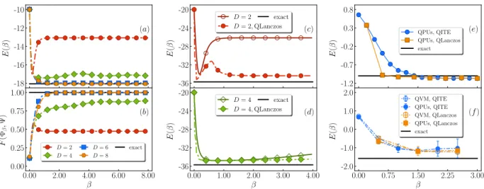
Figs.2and3show the energy obtained by QITE as a func-tion ofβandDfor the various models. As we increaseD, the asymptotic (β → ∞) energies rapidly converge to the exact
-18 -16 -14 -12 -10 E ( β ) (a) 0.00 2.00 4.00 6.00 8.00 β 0.00 0.25 0.50 0.75 1.00 F (Φ β , Ψ ) (b) D= 2 D= 4 D= 6 D= 8 exact -36 -32 -28 -24 -20 E ( β ) (c) D= 2 D= 2,QLanczos exact 0.00 1.00 2.00 3.00 4.00 β -36 -32 -28 -24 -20 E ( β ) (d) D= 4 D= 4,QLanczos exact -1.2 -0.7 -0.2 0.3 0.8 E ( β ) (e) QPUs, QITE QPUs, QLanczos exact 0.00 0.75 1.50 2.25 3.00 β -2.0 -1.0 0.0 1.0 2.0 E ( β ) (f) QVM, QITE QPUs, QITE QVM, QLanczos QPUs, QLanczos exact
FIG. 2: Left: QITE energyE(β)(a) and fidelityF (b) between finite-time stateΦ(β)and exact ground stateΨas function of imaginary time
β, for a 1D 10-site Heisenberg model, showing the convergence with increasing unitary domains ofD= 2−8qubits. Middle: QITE (dashed red, dot-dashed green lines) and QLanczos (solid red, solid green lines) energies as function of imaginary timeβ, for a 1D Heisenberg model withN = 20qubits, using domains ofD= 2(c) and4qubits (d), showing improved convergence of QLanczos over QITE. Black line is the exact ground-state energy/fidelity. Right: QITE and QLanczos energyE(β)as a function of imaginary timeβfor (e) 1-qubit field model using the QVM and QPU (qubit 14 on Aspen-1), (f) 2-qubit AFM transverse field Ising model using the QVM and QPU (qubit 14, 15 on Aspen-1). Black line is the exact ground-state energy (see SI for details).
ground-state. For smallD, the inexact QITE tracks the exact QITE for a time until the correlation length exceedsD. Af-terwards, it may go down or up. The non-monotonic behavior is strongest for small domains; in the MAXCUT example, the smallest domainD = 2gives an oscillating energy; the first point at which the energy stops decreasing is a reasonable es-timate of the ground-state energy. In all models, increasing
Dpast a maximum value (less thanN) no longer affects the asymptotic energy, showing that the correlations have satu-rated (this is true even in the MAXCUT instance).
Figs. 2e and2f show the results of running the QITE al-gorithm on Rigetti’s QVM and Aspen-1 QPUs for 1- and 2-qubits, respectively. The error bars are due to gate, readout, incoherent and cross-talk errors. Sufficient samples were used to ensure that sampling error is negligible. Encouragingly for near-term simulations, despite these errors it is possible to converge to a ground-state energy close to the exact energy for the 1-qubit case. This result reflects a robustness that is some-times informally observed in imaginary time evolution algo-rithms in which the ground state energy is approached even if the imaginary time step is not perfectly implemented. In the 2-qubit case, although the QITE energy converges, there is a systematic shift which is reproduced on the QVM using available noise parameters for readout, decoherence and de-polarizing noise [31]. Remaining discrepancies between the emulator and hardware are likely attributable to cross-talk be-tween parallel gates not included in the noise model (see SI). However, reducing decoherence and depolarizing errors in the QVM or using different sets of qubits with improved noise characteristics (see SI) all lead to improved convergence to the exact ground-state energy.
Quantum Lanczos algorithm. Given the QITE subroutine,
0 1 2 3 4 β -5 -4 -3 -2 -1 E ( β ) (a) D= 2 D= 4 D= 6 exact 0 2 4 6 8 β (b) D= 2 D= 4 exact 0 4 8 12 16 β 0.00 0.25 0.50 0.75 1.00 P ( C = Cm a x ) (c) D= 2 D= 4 D= 6 exact 0.0 1.0 2.0 3.0 R[˚A] (d) β= 0 β= 1 β= 2 β= 3 exact -5 -4 -3 -2 -1 E ( β ) -1.2 -0.9 -0.6 -0.3 0.0 0.3 E ( β ) [EH a ]
FIG. 3: (a) QITE energyE(β)as a function of imaginary timeβ
for a 6-site 1D long-range Heisenberg model, for unitary domains
D = 2−6; (b) a 4-site 1D Hubbard model withU/t = 1, for unitary domainsD = 2,4. (c) Probability of MAXCUT detection,
P(C = Cmax) as a function of imaginary timeβ, for the6-site graph in the panel. (d) QITE energy for the H2molecule in the STO-6G basis as a function of bond-lengthR andβ. Black line is the exact ground-state energy/probability of detection.
we now consider how to formulate a quantum Lanczos al-gorithm, which is an especially economical realization of a quantum subspace method [32,33]. An important practical motivation is that the Lanczos algorithm typically converges much more quickly than imaginary time evolution, and often in physical simulations only tens of iterations are needed to converge to good precision. In addition, Lanczos provides a
0.0 1.0 2.0 3.0 4.0 β -1.80 -1.35 -0.90 -0.45 0.00 h ˆHi ( β ) (a) D= 2 D= 3 D= 4 D= 5 exact 1.0 2.0 3.0 4.0 β -1.10 -1.00 -0.90 -0.80 -0.70 h ˆHi ( β ) (b) QVM, noiseless QVM, with noise QPUs exact 1.0 2.0 3.0 4.0 β -1.80 -1.60 -1.40 -1.20 -1.00 h ˆHi ( β ) (c) Emulator, noise Emulator, noise exact
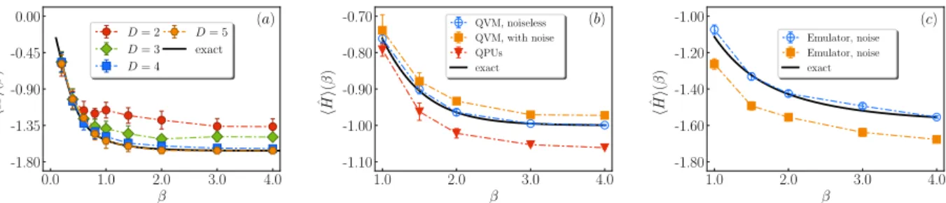
FIG. 4: Left: Thermal (Gibbs) averagehHˆiat temperatureβfrom QMETTS for a 1D 6-site Heisenberg model (exact emulation). Black line is the exact thermal average without sampling error. Middle, Right: Thermal averagehHˆiat temperatureβfrom QMETTS for (b) a 1 qubit field model using QVMs and QPUs, and (c) 2 qubit AFM transverse field Ising model using QVM.
natural way to compute excited states. Consider the sequence of imaginary time vectors|Φli=e−l∆τ
ˆ
H|Φi,l = 0,1, . . . n, wherecl =kΦlk. In QLanczos, we consider the vectors af-ter even numbers of time steps|Φ0i,|Φ2i. . . to form a ba-sis for the ground-state. (SI describes the equivalent treat-ment in terms of normalized imaginary time vectors). These vectors define an overlap matrix whose elements can be com-puted entirely from norms,Sll′ =hΦl|Φl′i=c2(l+l′)/2, where
c(l+l′)/2is the norm of another integer time step vector, and the overlap matrix elements forn/2vectors can be accumu-lated for free afternsteps of time evolution. The Hamilto-nian matrix elements satisfy the identityHll′ =hΦl|Hˆ|Φl′i=
hΦ(l+l′)/2|Hˆ|Φ(l+l′)/2i. Although the Hamiltonian has∼n2
matrix elements, there are only∼nunique elements, and im-portantly, each is a simple expectation value of the energy during the imaginary time evolution. This economy of ma-trix elements is a property shared with the classical Lanczos algorithm. Whereas the classical Lanczos iteration builds a Krylov space in powers ofHˆ, QLanczos builds a Krylov space in powers ofe−2∆τHˆ; in the limit of small∆τthese Krylov spaces are identical. Diagonalization of the QLanczos Hamil-tonian matrix is guaranteed to give a ground-state energy that is lower than that of the last imaginary time vectorΦn(while higher roots approximate excited states). Thus, as long as one is willing to take measurements of the energy during the imag-inary time evolution process, one can use QLanczos to gener-ate an improved ground stgener-ate (or excited stgener-ates).
With a limited computational budget, we can use inexact QITE to generate Φl, Φ′
l. However, in this case the above expressions forSll′andHll′in terms of expectation values are
no longer exactly satisfied which can create numerical issues (e.g. the overlap may no longer be positive). To handle this as well as errors due to noise and sampling in real experiments, the QLanczos algorithm needs to be stabilized by ensuring that successive vectors are not nearly linearly dependent (see SI).
We demonstrate the QLanczos algorithm using classical emulation on the 1D Heisenberg Hamiltonian, as used for the QITE algorithm in Fig. 2 (see SI). Using exact QITE (large domains) to generate matrix elements, quantum Lanc-zos converges much more rapidly than imaginary time evo-lution. Using inexact QITE (small domains), convergence is
usually faster and also reaches a lower energy. We also as-sess the feasibility of QLanczos in presence of noise, using emulated noise on the Rigetti QVM as well as on the Rigetti Aspen-1 QPUs. In Fig.2, we see that QLanczos also provides more rapid convergence than QITE with both noisy classical emulation as well as on the physical device for 1 and 2 qubits.
Quantum thermal averages. The QITE subroutine can be
used in a range of other algorithms. For example, we discuss how to compute thermal averagesTrˆ
Oe−βHˆ /Tr
e−βHˆ
us-ing imaginary time evolution. Several procedures have been proposed for quantum thermal averaging, ranging from gen-erating the finite-temperature state explicitly by equilibration with a bath [34], to a quantum analog of Metropolis sam-pling [35] that relies on phase estimation, as well as meth-ods based on ancilla based Hamiltonian simulation with post-selection [36] and approaches based on recovery maps [37]. However, given a method for imaginary time evolution, one can generate thermal averages of observables without any ancillae or deep circuits. This can be done by adapting to the quantum setting the classical minimally entangled typical thermal state (METTS) algorithm [19,20], which generates a Markov chain from which the thermal average can be sam-pled. The QMETTS algorithm can be carried out as follows (i) start from a product state, carry out imaginary-time evolution (using QITE) up to timeβ(ii) measure the expectation value of the observable that one wants to produce a thermal aver-age for (iii) measure a product operator such asZˆ1Zˆ2. . .ZˆN, to collapse back onto a random product state (iv) repeat (i). Note that in step (iii) one can measure in any product basis, and randomizing the product basis can be used to reduce the autocorrelation time and avoid ergodicity problems in sam-pling.
In Fig. 4we show the results of quantum METTS (using exact classical emulation) for the thermal averagehHˆi as a function of temperatureβ, for the 6-site Heisenberg model for several temperatures and domain sizes; sufficiently large
Dconverges to the exact thermal average at eachβ; error bars reflect only finite QMETTS samples. We also show an im-plementation of quantum METTS on the Aspen-1 QPU and QVM with a 1-qubit field model (Fig.4b), and using the QVM for a 2-qubit AFM transverse field Ising model (Fig.4c).
imaginary time evolution (QITE) and the Lanczos algorithm (QLanczos), that can be carried out without ancillae or deep circuits, and which, for bounded correlation length, achieve exponential reductions in space and time per iteration rela-tive to their classical counterparts. They provide new quan-tum routes to approximate ground-states of Hamiltonians in both physical simulations and in optimization that avoid some of the current disadvantages of phase estimation based ap-proaches and variational algorithms. The QLanczos itera-tion appears especially powerful if sufficient sampling can be done, as in practice it obtains accurate estimates of ground-states from only a few iterations, and also provides an estimate of excited states. Additionally, further algorithms that use QITE and QLanczos as subroutines can be formulated, such as the quantum minimally entangled thermal states algorithm to compute thermal averages. Encouragingly, these algorithms appear useful in conjunction with near-term quantum archi-tectures, and serve to demonstrate the power of quantum el-evations of classical simulation techniques, in the continuing search for quantum supremacy.
Author contributions. MM, CS, GKC designed the
algo-rithms. FGSLB established the mathematical proofs and error estimates. EY and MJO’R performed classical tensor network simulations. MM, CS, ATKT carried out classical exact emu-lations. ATKT and AJM designed and carried out the Rigetti QVM and QPUs experiments. All authors contributed to the discussion of results and writing of the manuscript.
Acknowledgments. MM, GKC, FGSLB, ATKT, AJM
were supported by the US NSF via RAISE-TAQS CCF 1839204. MJO’R was supported by an NSF graduate fellow-ship via grant No. DEG-1745301; the tensor network algo-rithms were developed with the support of the US DOD via MURI FA9550-18-1-0095. EY was supported by a Google fellowship. CS was supported by the Simons Collaboration on the Many-Electron Problem. The Rigetti computations were made possible by a generous grant through Rigetti Quan-tum Cloud services supported by the CQIA-Rigetti Partner-ship Program. We thank GH Low, JR McClean, R Babbush for discussions, and the Rigetti team for help with the QVM and QPU simulations.
SUPPLEMENTAL INFORMATION
Representing imaginary-time evolution by unitary maps
As discussed in the main text, we map the scaled non-unitary action of e−∆τˆhm on a state Ψ to that of a unitary
e−i∆τAˆ[m], i.e.
|Ψ′i ≡c−1/2e−∆τˆhm|Ψi=e−i∆τAˆ[m]|Ψi . (6) wherec =hΨ|e−2∆τˆhm|Ψi. ˆh
macts onkqubits;Aˆis Her-mitian and acts on a domain ofDqubits around the support ofˆhm, and is expanded as a sum of Pauli strings acting on the
Dqubits, ˆ A[m] = X i1i2...iD a[m]i1i2...iDσi1σi2. . . σiD =X I a[m]IσI (7)
where I denotes the index i1i2. . . iD. Define |∆0i =
|Ψ′i−|Ψi
∆τ and|∆i = −iAˆ[m]|Ψi. Our goal is to minimize the difference||∆0−∆||. If the unitarye−i∆τAˆ[m]is defined over a sufficiently large domainD(related to the correlation length of|Ψi, see Section ) then this error minimizes at∼0, for small∆τ. Minimizing for reala[m]corresponds to mini-mizing the quadratic functionf(a[m])
f(a[m]) =f0+ X I bIa[m]I+ X IJ a[m]ISIJa[m]J (8) where f0=h∆0|∆0i , (9) SIJ =hΨ|σ†IσJ|Ψi , (10) bI =ihΨ|σI†|∆0i −ih∆0|σI|Ψi , (11) whose minimum obtains at the solution of the linear equation
S+STa[m] =−b (12)
In general,S+STmay have a non-zero null-space. Thus, we
solve Eq. (12) either by applying the generalized inverse of
S+STor by an iterative algorithm such as conjugate gradient. For fermionic Hamiltonians, we replace the Pauli operators in Eq. (7) by fermionic field operators. For a number conserv-ing Hamiltonian, such as the fermionic Hubbard Hamiltonian treated in Fig. 3 in the main text, we write
ˆ A[m] = X i1i2...iD a[m]i1i2...iDfˆ † i1. . . ˆ fiD/† 2 ˆ fiD/2+1. . .fˆiD (13) wherefˆ†,fˆare fermionic creation, annihilation operators re-spectively.
Rigorous Run Time Bounds
Here we present a more detailed analysis of the running time of the algorithm. Consider ak-local Hamiltonian
H = m
X
l=1
hl (14)
acting on ad-dimensional lattice withkhik ≤1, wherek∗kis the operator norm. In imaginary time evolution one typically applies Trotter formulae to approximate
e−βH|Ψ0i
for an initial state |Ψ0i(which we assume to be a product state) by
e−βh1/n. . . e−βhm/nn|Ψ0i k e−βh1/n. . . e−βhm/nn|Ψ0ik
. (16)
This approximation leads to an error which can be made as small as one wishes by increasing the number of time stepsn. Let |Ψsi be the state (after renormalization) obtained by applyingstermse−thi/nfrom e−th1/n. . . e−thm/nn; with
this notation|Ψmniis the state given by Eq. (16). In the QITE algorithm, instead of applying each of the operatorse−thi/n to|Ψ0i(and renormalizing the state), one applies local uni-tariesUswhich should approximate the action of the original operator. Let|Φsibe the state aftersunitaries have been ap-plied.
LetCbe an upper bound on the correlation length of|Ψsi for everys: we assume that for every s, and every pair of observablesAandBseparated by dist(A, B)sites,
Cs(A, B) =hΨs|A⊗B|Ψsi − hΨs|A|ΨsihΨs|B|Ψsi
≤ kAkkBke−dist(A,B)/C.
(17)
Theorem 1. For every ε > 0, there are unitaries Us each
acting on
k(2C)dlnd(2√2nmε−1) (18)
qubits such that
k|Ψmni − |Φmnik ≤ε (19)
Proof. We have
k|Ψsi − |Φsik=k|Ψsi −Us|Φs−1ik
≤ k|Ψsi −Us|Ψs−1ik+k|Ψs−1i − |Φs−1ik. (20) To bound the first term we use our assumption that the corre-lation length of|Ψs−1iis smaller thanC. Consider a region
Rv of all sites that are a distance at mostv (in the Manhat-tan disManhat-tance on the lattice) of the sites in whichhis acts. Let tr\Rv(|ΨsihΨs|)be the reduced state onRv, obtained by par-tial tracing over the complement ofRvin the lattice. Since
|Ψsi= e −βhis/n|Ψs −1i ke−βhis/n|Ψ s−1ik , (21)
it follows from Eq. (17) and Lemma 9 of [38] that
tr\Rv(|ΨsihΨs|)−tr\Rv(|Ψs−1ihΨs−1|) 1 ≤ kehis/nk−1e−Cv ≤2e−Cv, (22)
where we used that for n ≥ 2β, ke−βhis/nk ≥ kI −
βhis/nk ≥1−β/n≥1/2. Abovek ∗ k1is the trace norm. The key result in our analysis is Uhlmann’s theorem (see e.g. Lemmas 11 and 12 of [38]). It says that two pure states
with nearby marginals must be related by a unitary on the pu-rifying system. In more detail, if|ηiAB and|νiAB are two states s.t. kηA −νAk1 ≤ δ, then there exists a unitary V acting onBs.t.
k|ηiAB−(I⊗V)|νiABk ≤2
√
δ. (23)
Applying Uhlmann’s theorem to |Ψsi and |Ψs−1i, with
B=Rv, and using Eq. (22), we find that there exists a unitary
Usacting onRvs.t.
k|Ψsi −Us|Ψs−1ik ≤2
√
2e−2vC, (24) which by Eq. (20) implies
k|Ψnmi − |Φnmik ≤2
√
2mne−2vC, (25) Choosingν= 2Cln(2√2nmε−1)as the width of the sup-port of the approximating unitaries, the error term above isε. The support of the local unitaries iskνdqubits (as this is an upper bound on the number of qubits inRν). Therefore each unitaryUsacts on at most
k(2C)dlnd(2√2nmε−1) (26) qubits.
FindingUs: In the algorithm we claim that we can find the unitariesUs by solving a least-square problem. This is in-deed the case if we can write them asUs = eiA[s]/n with
A[s]a Hamiltonian of constant norm. Then for sufficiently largen,Us=I+iA[s]/n+O((1/n)2)and we can findA[s] by performing tomography of the reduced state over the re-gion whereUsacts and solving the linear problem given in the main text. Because we apply Uhlmann’s Theorem to|Ψs−1i and e−βhis/n|Ψ s−1i ke−βhis/n|Ψs−1ik, (27) usinge−βhis/n = I−βh is/n+O((1/n)2)and following the proof of the Uhlmann’s Theorem, we find that the unitary can indeed be taken to be close to the identity, i.e.Uscan be written aseiA[s]/n.
Total Run Time: Theorem 1 gives an upper bound on the maximum support of the unitaries needed for a Trotter up-date, while tomography of local reduced density matrices gives a way to find the unitaries. The cost for tomography is quadratic in the dimension of the region, so it scales as exp(O(k(2C)dlnd(2√2nmε−1))). This is also the cost to solve classically the linear system which gives the associated HamiltonianA[s] and of finding a circuit decomposition of
Us=eiA[s]/nin terms of two qubit gates. As this is repeated
mntimes, for each of themnterms of the Trotter decompo-sition, the total running time (of both quantum and classical parts) is
This is exponential inCd, withCthe correlation length, and quasi-polynomial inn (the number of Trotter steps) andm
(the number of local terms in the Hamiltonian. Note that typ-icallym=O(N), withNthe number of sites). While this an exponential improvement over the exp(O(N)) scaling clas-sically, the quasi-polynomial dependence on m can still be prohibitive in practice. Below we show how to improve on that.
Local Approximation: If one is only interested in a local ap-proximation of the state (meaning that all the local marginals of|Φnmiare close to the ones ofe−βH|Ψ0i, but not neces-sarily the global states), then the support of the unitaries be-comes independent of the number of terms of the Hamiltonian
m(while for global approximation we have a polylogarithmic dependence onm):
Theorem 2. For every ε > 0, there are unitaries Us each
acting on
k(2C)dlnd2√2n(|S|+Cln(8nC(2C)d+1ε−1)d (29)
qubits such that for every connected regionSof size at most
|S|,
tr\S(|ΨmnihΨmn|)−tr\S(|ΦmnihΦmn|)1≤ε
Proof. Consider the unitariesUsobtained in the proof of
The-orem1satisfying Eq. (24).
Consider the replacement of the local term of the Trotter expansion by the unitary Us for all local terms which are more than 2Clog(1/δ) sites away from the regionS. Be-cause the correlation length is always smaller thanC, we find by Lemma 9 of [38] that the total error on the reduced density matrix in regionScan be bounded as
n
Z ∞
2Cln(1/δ)
e−l/2Clddl≤4nC(2C)d+1δ. (30) For the local terms which are at most a distance 2Clog(1/δ) from the region S, in turn, the total error is bounded by the sum of each individual term, giving:
(|S|+Clog(1/δ))dn2√2e− ν
2C (31)
Choosing δ = ε/(8nC(2C)d+1) and ν = 2Cln(2√2n(|S| + Cln(8nC(2C)d+1ε−1)d) gives the result.
Non-Local Terms: Suppose the Hamiltonian has a termhq acting on qubits which are not nearby, e.g. on two sitesiand
j. Thene−βhq/ncan still be replaced by a unitary, which only acts on sitesiandj and qubits in the neighborhoods of the two sites. This is the case if we assume that the state has a fi-nite correlation length and the proof is again an application of Uhlmann’s theorem (we follow the same argument from the
proof of Theorem1 but defineRv in that case as the union of the neighborhoods ofiandj). Note however that the as-sumption of a finite correlation length might be less natural for models with long range interactions.
Scaling with temperature and increase of correlation length:
Our discussion has been based on the assumption that the cor-relation lengthCis small on all intermediate states. Here we discuss the range of validity of the assumption.
Let us begin with an example where the correlation length can increase very quickly with number of local terms applied (this was communicated to us by Guang Hao Low). Con-sider a projection on two qubitsPi,i+1 =|0,0ih0,0|i,i+1+
|1,1ih1,1|i,i+1. Then
P1,2P2,3. . . Pn−1,n|+i⊗n, (32) with|+i = (|0i+|1i)/p
(2), is the GHZ state(|0. . .0i+
|1. . .1i)/√2, which has correlation lengthC = n. While the projectorPi,i+1cannot appear as a local terme−βh1/nin the Trotter decomposition, this example show that we cannot expect a speed-of-sound bound on the spread of correlations for a circuit with non-unitary gates; indeed the example shows a depth two circuit can already create long range correlations. However, we expect that generically the correlations do grow ballistically. Consider the state
|ψni:=
e−βh1/n. . . e−βhm/nn|Ψ0i
k e−βh1/n. . . e−βhm/nn|Ψ0ik. (33)
afternrounds have been applied. Let us assume the Hamil-tonian acts on a line, is translation invariant and has nearest-neighbor interactions. Then the state is a matrix product state of bond dimension at most2n. For matrix product states we can bound the correlations as follows (see e.g. Lemma 22 of [38])
Cs(A, B) =hΨs|A⊗B|Ψsi − hΨs|A|ΨsihΨs|B|Ψsi
≤ kAkkBk22ne−∆dist(A,B).
(34) where we define the gap of the matrix-product-state as∆ := 1−λ, withλthe second largest eigenvalue of the transfer ma-trix of the mama-trix product state (normalized so that the largest eigenvalue is one). In the GHZ example above, the gap∆ = 0 and that is the reason for the fast build up of correlations. Typ-ically we expect the gap to be independent ofnor decrease mildly as1/poly(n).
From the above, we can replace a non-unitary local Trotter term applied to|ψniby an unitary acting onO(n/∆)qubits. Takingn = O(β)to reach temperatureβ in the imaginary time evolution, the support of the unitaries would scale as
O(β/∆). Assuming∆is a constant, we find a linear increase in temperature.
We also expect the linear growth of correlations/unitary support with inverse temperature also to hold generically in two dimensions, although there the analysis is more subtle as
rigorous results for the expected behaviour of the transfer erator (which becomes a one-dimensional tensor product op-erator) and its gap are not available.
Spreading of correlations
In the main text, we argued that the correlation volumeV of the statee−βH|Ψiis bounded for many physical Hamiltonians and saturates at the ground-state withV ≪NwhereNis the system size. To numerically measure correlations, we use the mutual information between two sites, defined as
I(i, j) =S(i) +S(j)−S(i, j) (35) whereS(i)is the von Neumann entropy of the density matrix of sitei(ρ(i)) and similarly forS(j), andS(i, j)is the von Neumann entropy of the two-site density matrix for sitesiand
j(ρ(i, j)).
To compute the mutual information in Fig. 1 in the main text, we used matrix product state (MPS) and finite projected entangled pair state (PEPS) imaginary time evolution for the spin-1/21D and 2D FM transverse field Ising model (TFI)
HT F I =− X hiji σizσzj −h X i σix (36)
where the sum overhi, ji pairs are over nearest neighbors. We use the parameterh = 1.25for the 1-D calculation and
h= 3.5for the 2-D calculations as the ground-state is gapped in both cases. It is known that the ground-state correlation length is finite.
MPS. We performed MPS imaginary time evolution (ITE) on a 1-D spin chin withL= 50sites with open boundary condi-tions. We start from an initial state that is a random product state, and perform ITE using time evolution block decimation (TEBD) [39,40] with a first order Trotter decomposition. In this algorithm, the Hamiltonian is separated into terms oper-ating on even and odd bonds. The operators acting on a single bond are exponentiated exactly. One time step is given by time evolution of odd and even bonds sequentially, giving rise to a Trotter error on the order of the time step∆τ. In our calculation, a time step of∆τ = 0.001was used.
We carry out ITE simulations with maximum bond dimen-sion ofD = 80, but truncate singular values less than 1.0e-8 of the maximum singular value. In the main text, the ITE re-sults are compared against the ground state obtained via the density matrix renormalization group (DMRG)). This should be equivalent to comparing to a long-time ITE ground state. The long-time ITE (β = 38.352) ground state reached an ergy per site of -1.455071, while the DMRG ground-state en-ergy per site is−1.455076. The relative error of the nearest neighbor correlations is on the order of 10−4 to10−3, and about10−2for correlations between the middle site and the end sites (a distance of 25 sites). The error in fidelity between the two ground states was about5×10−4.
PEPS. We carried out finite PEPS [41–44] imaginary time evolution for the two-dimensional transverse field Ising model on a lattice size of21×31. The size was chosen to be large enough to see the spread of mutual information in the bulk without significant effects from the boundary. The mutual in-formation was calculated along the long (horizontal) axis in the center of the lattice. The standard Trotterized imaginary time evolution scheme for PEPS [45] was used with a time step∆τ = 0.001, up to imaginary time β = 6.0, starting from a random product state. To reduce computational cost from the large lattice size, the PEPS was defined in a transla-tionally invariant manner with only 2 independent tensors [46] updated via the so-called “simple update” procedure [47]. The simple update has been shown to be sufficiently accurate for capturing correlation functions (and thusI(i, j)) for ground states with relatively short correlation lengths (compared to criticality) [48,49]. We chose a magnetic field valueh= 3.5 which is detuned from the critical field (h≈ 3.044) but still maintains a correlation length long enough to see interesting behaviour.
Accuracy:Even though the simple update procedure was used for the tensor update, we still needed to contract the21×31 PEPS at at every imaginary time stepβ for a range of corre-lation functions, amounting to a large number of contractions. To control the computational cost, we limited our bond di-mension toD= 5and used an optimized contraction scheme [50], with maximum allowed bond dimension ofχ= 60 dur-ing the contraction. Based on converged PEPS ground state correlation functions with a larger bond dimension ofD= 8, ourD = 5 PEPS yields I(i, i+r)(wherer denotes hori-zontal separation) at largeβwith a relative error of≈1%for
r= 1−4,5%or less forr= 5−8, and10%or greater for
r >8. At smaller values ofβ (<0.5) the errors up tor= 8 are much smaller because the bond dimension of 5 is able to completely support the smaller correlations (see Fig. 1, main text). While error analysis on the 2D Heisenberg model [48] suggests that errors with respect toD = ∞may be larger, such analysis also confirms that aD = 5PEPS captures the qualitative behaviour of correlation in the ranger = 5−10 (and beyond). Aside from the bond dimension error, the pre-cision of the calculations is governed byχand the lattice size. Using the21×31lattice andχ = 60, we were able to con-verge entries of single-site density matricesρ(i)to a precision of±10−6(two site density matrices ρ(i, j)had higher pre-cision). Forβ = 0.001−0.012, the smallest eigenvalue of
ρ(i)fell below this precision threshold, leading to significant noise inI(i, j). Thus, these values ofβare omitted from Fig. 1 (main text) and the smallest reported values ofIare10−6, although with more precision we expectI→0asr→ ∞.
Finally, the energy and fidelity errors were computed with respect to the PEPS ground stateof the same bond dimension
atβ= 10.0(10000 time steps). The convergence of the quan-tities shown in Fig. 1 (main text) thus isolates the convergence of the imaginary time evolution, and does not include effects of other errors that may result from deficiencies in the wave-function ansatz.
Simulation models
We here define, and give some background on, the models used in the QITE and QLanczos simulations.
1 qubit field model
ˆ
H =αXˆ+βZˆ (37)
This Hamiltonian has previously been used as a model for quantum simulations on physical devices in Ref. [30].We used
α= √1
2 andβ = 1
√
2. In simulations with this Hamiltonian, the qubit is assumed to be initialized in theZ basis.
1D Heisenberg and transverse field Ising model
The 1D short-range Heisenberg Hamiltonian is defined as ˆ
H =X
hiji
ˆ
Si·Sˆj , (38)
the 1D long-range Heisenberg Hamiltonian as ˆ
H=X
i6=j 1
|i−j|+ 1Sˆi·Sˆj , (39) and the AFM transverse-field Ising Hamiltonian as
ˆ H =X hiji ˆ SizSˆjz+ X i hSˆix . (40) 1D Hubbard model
The 1D Hubbard Hamiltonian is defined as ˆ H =−X hijiσ a†iσajσ+U X i ˆ ni↑nˆi↓ (41)
whereˆniσ =a†iσaiσ,σ∈ {↑,↓}, andh·idenotes summation over nearest-neighbors, here with open-boundary conditions. We label the n lattice sites with an indexi = 0. . . n−1, and the2n−1basis functions as|ϕ0i=|0 ↑i,|ϕ1i=|0 ↓
i,|ϕ2i = |1 ↑i, |ϕ3i = |1 ↓i . . .. Under Jordan-Wigner transformation, recalling that
ˆ np= 1−Zp 2 , ˆ a†pˆaq+ ˆa†qˆap= XpXqQpk−=q1+1Zk(1−ZpZq) 2 , (42)
withp= 0. . .2n−2andq < p, the Hamiltonian takes the form ˆ H =−X p XpXp+2Zp+1(1−ZpZp+2) 2 +U X peven (1−Z2i)(1−Z2i+1) 4 +µ X p (1−Zp) 2 (43)
H2molecule minimal basis model
We use the hydrogen molecule minimal basis model at the STO-6G level of theory. This is a common minimal model of hydrogen chains [51, 52] and has previously been stud-ied in quantum simulations, for example in [29]. Given a molecular geometry (H-H distanceR) we perform a restricted Hartree-Fock calculation and express the second-quantized Hamiltonian in the orthonormal basis of RHF molecular or-bitals as [53] ˆ H =H0+ X pq hpqˆa†paˆq+1 2 X prqs vprqsˆa†pˆa†qˆasˆar (44)
wherea†,aare fermionic creation and annihilation operators for the molecular orbitals.
The Hamiltonian (44) is then encoded by a Bravyi-Kitaev transformation into the 2-qubit operator
ˆ
H=g0I⊗I+g1Z⊗I+g2I⊗Z+g3Z⊗Z+g4X⊗X+g5Y⊗Y , (45) with coefficientsgigiven in Table I of [29].
MAXCUT Hamiltonian
The MAXCUT Hamiltonian encodes the solution of the MAXCUT problem. Given a graphΓ = (V, E), whereV
is a set of vertices andE ⊆V ×V is a set of links between vertices inV, a cut ofΓis a subsetS⊆V ofV. The MAX-CUT problem consists in finding a cutSthat maximizes the number of edges betweenS andSc (the complement ofS). We denote the number of links in a given cutSasC(S).
In Figure 3 of the main text, we consider a graph Γ with vertices V = {0,1,2,3,4,5} and links E =
{(0,3),(1,4),(2,3),(2,4),(2,5),(4,5)}. It is easy to ver-ify that S = {0,2,4}, {0,1,2}, {3,4} and their comple-mentsScare solutions of the MAXCUT problem, with weight
Cmax= 5.
The MAXCUT problem can be formulated as a Hamilto-nian ground-state problem, by (i) associating a qubit to every vertex inV, (ii) associating to every partitionS=an element of the computational basis (here assumed to be in thez direc-tion) of the form|z0. . . zn−1i, wherezi = 1 ifi ∈ S and
eigenvalue of the2-local Hamiltonian ˆ C=− X (ij)∈E 1−Sˆz iSˆjz 2 . (46)
The spectrum ofCˆis a subset of numbersC∈ {0,1. . .|E|}. In the present work, we initialize the qubits in the state
|Φi = |+i⊗n, where|+i = |0i√+|1i
2 , and evolve Φin imag-inary time. Measuring the evolved state at timeβ|Φ(β)iwill collapse it onto an element|z0. . . zn−1iof the computational basis, which is also an eigenfunction of Cˆ with eigenvalue
C. In Figure 3 in the main text, we illustrate the probabil-ityP(|C| = Cmax)that such measurements yield a MAX-CUT solution. Note that, even in the presence of oscillations (with the smallest domain size D = 2) this probability re-mains above60%.
Numerical simulation details QITE stabilization
Sampling noise in the expectation values of the Pauli oper-ators can affect the solution to Eq. (12) that sometimes lead to numerical instabilities. We regularizeS+ST against such
statistical errors by adding a smallδto its diagonal. To gener-ate the data presented in Figures 2 and 4 of the main text, we usedδ= 0.01for 1-qubit calculations andδ= 0.1for 2-qubit calculations.
QLanczos stabilization
In quantum Lanczos, we generate a set of wavefunctions for different imaginary-time projections of an initial state|Ψi, using QITE as a subroutine. The normalized states are
|Φli= e−l∆τHˆ|Ψ Ti ke−l∆τHˆΨ Tk ≡nle−l∆τ ˆ H |ΨTi 0≤l < Lmax . (47) where nl is the normalization constant. For the exact imaginary-time evolution andl,l′both even (or odd) the ma-trix elements
Sl,l′ =hΦl|Φl′i , Hl,l′ =hΦl|Hˆ|Φl′i (48)
can be computed in terms of expectation values (i.e. exper-imentally accessible quantities) only. Indeed, defining2r =
l+l′, we have Sl,l′ =nlnl′hΨT|e−l∆τ ˆ He−l′∆τHˆ |ΨTi= nlnl′ n2 r , (49) and similarly Hl,l′ =nlnl′hΨT|e−l∆τ ˆ HHeˆ −l′∆τHˆ |ΨTi= = nlnl′ n2 r h Φr|Hˆ|Φri=Sl,l′hΦr|Hˆ|Φri . (50)
The quantitiesnrcan be evaluated recursively, since 1 n2 r+1 =hΨT|e−(r+1)∆τ ˆ He−(r+1)∆τHˆ|Ψ Ti= =hΦr|e− 2∆τHˆ|Φ ri n2 r , (51)
For inexact time evolution, the quantitiesnrandhΦr|Hˆ|Φri can still be used to approximateSl,l′,Hl,l′.
Given these matrices, we then solve the generalized eigen-value equationHx = ESxto find an approximation to the
ground-state|Φ′i=P
lxl|Φlifor the ground state ofHˆ. This eigenvalue equation can be numerically ill-conditioned, asS
can contain small and negative eigenvalues for several reasons (i) asmincreases the vectors|Φlibecome linearly dependent; (ii) simulations have finite precision and noise; (iii)S,H are computed approximately when inexact time evolution is per-formed.
To regularize the problem, out of the set of time-evolved states we extract a better-behaved sequence as follows (i) start from|Φlasti = |Φ0i(ii) add the next|Φliin the set of time-evolved states s.t.|hΦl|Φlasti|< s, wheresis a regularization parameter0 < s < 1 (iii) repeat, setting the|Φlasti = Φl (obtained from (ii)), until the desired number of vectors is reached. We then solve the generalized eigenvalue equation
˜
Hx = ESx˜ spanned by this regularized sequence,
remov-ing any eigenvalues of S˜ less than a threshold ǫ. The
ex-act emulated QLanczos calculations reported in the main text were stabilized with this algorithm (the source of error here is primarily (iii)) using stabilization parameters= 0.95and
ǫ = 10−14. The stabilization parameters used in the QVM and QPU QLanczos calculations weres= 0.75andǫ= 10−2 (the main source of error in the simulations was (ii)). Note that the stabilization procedure is unlikely to fix all possible numerical instabilities, but was sufficient for all models and calculations performed in this work.
METTS algorithm
The METTS (minimally entangled typical thermal state) al-gorithm [54, 55] is a sampling method to calculate thermal properties based on imaginary time evolution. Consider the thermal average of an observableOˆ
hOˆi= 1 ZTr[e −βHˆOˆ] = 1 Z X i hi|e−βH/ˆ 2Oeˆ −βH/ˆ 2|ii (52) where{|ii}is an orthonormal basis set, andZis the partition function. Defining|φii=Pi−1/2e−β ˆ H/2 |ii, we obtain hOˆi= 1 Z X i Pihφi|Oˆ|φii (53) wherePi=hi|e−βH|ii. The summation in Eq.(53) can be es-timated by sampling|φiiwith probabilityPi/Z, and summing the sampledhφi|Oˆ|φii.
In standard Metropolis sampling for thermal states, one starts from |φii and obtains the next state |φji from ran-domly proposing and accepting based an acceptance proba-bility. However, rejecting and resetting in the quantum analog of Metropolis [56] is complicated to implement on a quantum computer, requiring deep circuits. The METTS algorithm pro-vides an alternative way to sample|φiidistributed with prob-abilityPi/Z without this complicated procedure. The algo-rithm is as follows
1. Choose a classical product state (PS)|ii.
2. Compute |φii = Pi−1/2e−βH/2|ii and calculate ob-servables of interest.
3. Collapse|φiito a new PS|i′iwith probabilityp(i →
i′) =|hi′|φii|2and repeat Step 2.
In the above algorithm,|φiiis named a minimally entan-gled typical thermal state (METTS). One can easily show that the set of METTS sampled following the above procedure has the correct Gibbs distribution [54]. Generally,{|ii}can be any orthonormal basis. For convenience when implementing METTS on a quantum computer,{|ii}are chosen to be prod-uct states.
On a quantum emulator or a quantum computer, the METTS algorithm is carried out as following
1. Prepare a product state|ii.
2. Imaginary time evolve|iiwith the QITE algorithm to
|φii =Pi−1/2e−βH/2|ii, and measure the desired ob-servables.
3. Collapse|φiito another product state by measurement. In practice, to avoid long statistical correlations between samples, we used the strategy of collapsing METTS onto al-ternating basis sets [54]. For instance, for the odd METTS steps,|φiiis collapsed onto theX-basis (assuming aZ com-putational basis, tensor products of|+iand|−i), and for the even METTS steps,|φiiis collapsed onto theZ-basis (tensor products of|0iand|1i). The statistical error is then estimated by block analysis [57].
Implementation on emulator and quantum processor
We used pyQuil, an open source Python library, to express quantum circuits that interface with both Rigetti’s quantum virtual machine (QVM) and the Aspen-1 quantum processing units (QPUs).
pyQuil provides a way to include noise models in the QVM simulations. Readout error can be included in a high-level API provided in the package and is characterized byp00(the probability of reading|0igiven that the qubit is in state|0i) andp11 (the probability of reading|1igiven that the qubit is in state|1i). Readout errors can be mitigated by estimating
the relevant probabilities and correcting the estimated expec-tation values. We do so by using a high level API present in pyQuil. A general noise model can also be applied to a gate in the circuit by applying the appropriate Kraus maps. Included in the package is a high level API that applies the same deco-herence error attributed to energy relaxation and dephasing to every gate in the circuit. This error channel is characterized by the relaxation time T1 and coherence timeT2. We also include in our emulation our own high-level API that applies the same depolarizing noise channel to every single gate by using the appropriate Kraus maps. The depolarizing noise is characterized byp1, the depolarizing probability for single-qubit gates andp2, the depolarizing probability for two-qubit gates. We do not include all sources of error in our emula-tion. We applied the same depolarizing and dephasing chan-nels to each gate operation for all qubits, when in reality, they can vary from qubit to qubit. In addition, noise due to cross-talk between qubits cannot be modeled using the QVM and is another source of discrepancy between the QVM and QPU results.
We investigate the influence of noise on the 2-qubit results obtained via the QVM using different noise parameters; Noise model 1:p00= 0.95,p11= 0.95,T1= 10.5µs,T2= 14.0µs,p1 = 0.001,p2=0.01, Noise model 2:p00= 0.99,p11= 0.99,T1= 10.5µs,T2=14.0µs,p1= 0.001,p2= 0.01 and, Noise model 3: p00 = 0.99, p11 = 0.99, T1 = 20.0µs, T2 =40.0µs, p1 = 0.0001,p2=0.001. Noise model 1 reflects realistic parameters that characterize the Aspen-1 QPUs we run our calculations on;p00,p11,T1, andT2 are reported values whereasp1 and
p2are values typically used to benchmark error mitigation al-gorithms [58]. We repeated 10 calculations for each noise model and note there is practically no variation from run to run. Fig.5(a) shows that reducing the readout error does not greatly affect the converged ground state energy after read-out error mitigation has been performed. However, reducing the other sources of error does improve the converged energy. Note that sufficient measurement samples are used such that the sampling variance is smaller than that due to noise.
We also ran 2-qubit simulations on different pairs of qubits on Aspen-1, with Q1 consisting of qubits 14, 15 and Q2 con-sisting of qubits 0, 1. These two pairs are reported to have different noise characteristics; Q1:p00= 0.95,p11= 0.95,T1 = 10.5µs,T2 =14.0µs, and, Q2: p00 = 0.90,p11 = 0.90,T1 = 6.5µs,T2=8.0µs. Based on this, we expect simulations on Q2 to be worse. Note that in contrast to our QVM calcula-tions, the results from the actual devices varied from run to run. Thus, we present the mean and standard deviation for 10 different runs on each pair. (Similarly, sufficient samples are taken when running the QVM such that the sampling variance is smaller than that due to noise). Fig.5(b) indeed demon-strates that Q2 provides a less faithful implementation of the quantum algorithm.
Parameters used in QVM and QPUs simulations
In this section, we include the parameters used in our QPU and QVM simulations. Note that all noisy QVM simulations (unless stated otherwise in the text) were performed with noise parameters from noise model 1. We also indicate the number of samples used during measurements for each Pauli operator.
TABLE I: QPUs: 1-qubit QITE and QLanczos.
Trotter stepsize nSamples δ s ǫ
0.2 100000 0.01 0.75 10−2
TABLE II: QPUs: 2-qubit QITE and QLanczos.
Trotter stepsize nSamples δ s ǫ
0.5 100000 0.1 0.75 10−2
TABLE III: QPUs: 1-qubit METTS.
β Trotter stepsize nSamples nMETTs δ
1.5 0.15 1500 70 0.01
2.0 0.20 1500 70 0.01
3.0 0.30 1500 70 0.01
4.0 0.40 1500 70 0.01
TABLE IV: QVM: 2-qubit QITE and QLanczos.
Trotter stepsize nSamples δ s ǫ
0.5 100000 0.1 0.75 10−2
TABLE V: QVM: 1-qubit METTS.
β Trotter stepsize nSamples nMETTs δ
1.0 0.10 1500 70 0.01
1.5 0.15 1500 70 0.01
2.0 0.20 1500 70 0.01
3.0 0.30 1500 70 0.01
4.0 0.40 1500 70 0.01
TABLE VI: QVM: 2-qubit METTS.
β Trotter stepsize nSamples nMETTs δ
1.0 0.10 30000 100 0.1 1.5 0.15 30000 100 0.1 2.0 0.20 30000 100 0.1 3.0 0.30 30000 100 0.1 4.0 0.40 30000 100 0.1 ∗
Corresponding author:[email protected] †
Corresponding author:[email protected]
[1] R. P. Feynman, “Simulating physics with computers,” Interna-tional Journal of Theoretical Physics, vol. 21, no. 6, pp. 467– 488, 1982.
[2] D. S. Abrams and S. Lloyd, “Simulation of many-body Fermi systems on a universal quantum computer,” Phys. Rev. Lett., vol. 79, pp. 2586–2589, 1997.
[3] S. Lloyd, “Universal quantum simulators,”Science, vol. 273, no. 5278, pp. 1073–1078, 1996.
[4] A. Aspuru-Guzik, A. D. Dutoi, P. J. Love, and M. Head-Gordon, “Simulated quantum computation of molecular ener-gies,”Science, vol. 309, no. 5741, pp. 1704–1707, 2005.
[5] A. Kandala, A. Mezzacapo, K. Temme, M. Takita, M. Brink, J. M. Chow, and J. M. Gambetta, “Hardware-efficient varia-tional quantum eigensolver for small molecules and quantum magnets,”Nature, vol. 549, pp. 242 EP –, Sep 2017.
[6] A. Kandala, K. Temme, A. D. Corcoles, A. Mezzacapo, J. M. Chow, and J. M. Gambetta, “Extending the computa-tional reach of a noisy superconducting quantum processor,”
arXiv:1805.04492, 2018.
[7] J. Kempe, A. Kitaev, and O. Regev, “The complexity of the local Hamiltonian problem,” SIAM Journal on Computing, vol. 35, no. 5, pp. 1070–1097, 2006.
[8] E. Farhi, J. Goldstone, S. Gutmann, and M. Sipser, “Quantum computation by adiabatic evolution.” MIT-CTP-2936, 2000.
[9] A. Y. Kitaev, “Quantum measurements and the abelian stabi-lizer problem,” 1995.
[10] E. Farhi, J. Goldstone, S. Gutmann, and M. Sipser, “A quantum approximate optimization algorithm.” MIT-CTP-4610, 2014.
[11] J. S. Otterbach, R. Manenti, N. Alidoust, A. Bestwick, M. Block, B. Bloom, S. Caldwell, N. Didier, E. S. Fried, S. Hong, P. Karalekas, C. B. Osborn, A. Papageorge, E. C. Peterson, G. Prawiroatmodjo, N. Rubin, C. A. Ryan, D. Scara-belli, M. Scheer, E. A. Sete, P. Sivarajah, R. S. Smith, A. Staley, N. Tezak, W. J. Zeng, A. Hudson, B. R. Johnson, M. Reagor, M. P. da Silva, and C. Rigetti, “Unsupervised machine learning on a hybrid quantum computer,” 2017.
[12] N. Moll, P. Barkoutsos, L. S. Bishop, J. M. Chow, A. Cross, D. J. Egger, S. lipp, A. Fuhrer, J. M. Gambetta, M. Ganzhorn, A. Kandala, A. Mezzacapo, P. M¨oller, W. Riess, G. Salis, J. Smolin, I. Tavernelli, and K. Temme, “Quantum optimization using variational algorithms on near-term quantum devices,”
Quantum Science and Technology, vol. 3, no. 3, p. 030503, 2018.
[13] A. Peruzzo, J. McClean, P. Shadbolt, M.-H. Yung, X.-Q. Zhou, P. J. Love, A. Aspuru-Guzik, and J. L. O’Brien, “A variational eigenvalue solver on a photonic quantum processor,” Nature Communications, 2014.
[14] J. R. McClean, J. Romero, R. Babbush, and A. Aspuru-Guzik, “The theory of variational hybrid quantum-classical al-gorithms,”New Journal of Physics, vol. 18, no. 2, p. 023023, 2016.
[15] H. R. Grimsley, S. E. Economou, E. Barnes, and N. J. Mayhall, “Adapt-vqe: An exact variational algorithm for fermionic simulations on a quantum computer,”arXiv preprint arXiv:1812.11173, 2018.
[16] J. R. McClean, S. Boixo, V. N. Smelyanskiy, R. Babbush, and H. Neven, “Barren plateaus in quantum neural network training landscapes,”arXiv preprint arXiv:1803.11173, 2018.
FIG. 5: QITE and QLanczos energyE(β)as a function of imaginary timeβfor 2-qubit simulations (a) using the QVM with different noise models, (b) Q1 and Q2 on Aspen-1.
“Variational quantum simulation of imaginary time evolution,” 2018.
[18] C. Lanczos, “An iteration method for the solution of the eigen-value problem of linear differential and integral operators,” J. Res. Natl. Bur. Stand. B, vol. 45, pp. 255–282, 1950.
[19] S. R. White, “Minimally entangled typical quantum states at finite temperature,”Phys. Rev. Lett., vol. 102, p. 190601, May 2009.
[20] E. M. Stoudenmire and S. R. White, “Minimally entangled typ-ical thermal state algorithms,”New Journal of Physics, vol. 12, no. 5, p. 055026, 2010.
[21] A. Uhlmann, “The “transition probability” in the state space of a*-algebra,” Reports on Mathematical Physics, vol. 9, no. 2, pp. 273–279, 1976.
[22] M. B. Hastings and T. Koma, “Spectral gap and exponential de-cay of correlations,”Communications in Mathematical Physics, vol. 265, no. 3, pp. 781–804, 2006.
[23] F. Verstraete and J. I. Cirac, “Mapping local Hamiltonians of fermions to local Hamiltonians of spins,” Journal of Statis-tical Mechanics: Theory and Experiment, vol. 2005, no. 09, p. P09012, 2005.
[24] D. W. Berry, A. M. Childs, and R. Kothari, “Hamiltonian sim-ulation with nearly optimal dependence on all parameters,” in
Foundations of Computer Science (FOCS), 2015 IEEE 56th An-nual Symposium on, pp. 792–809, IEEE, 2015.
[25] G. Vidal, “Efficient simulation of one-dimensional quantum many-body systems,” Phys. Rev. Lett., vol. 93, p. 040502, Jul 2004.
[26] U. Schollw¨ock, “The density-matrix renormalization group in the age of matrix product states,”Annals of Physics, vol. 326, no. 1, pp. 96 – 192, 2011.
[27] N. Schuch, M. M. Wolf, F. Verstraete, and J. I. Cirac, “Com-putational complexity of projected entangled pair states,”Phys. Rev. Lett., vol. 98, p. 140506, 2007.
[28] J. Haferkamp, D. Hangleiter, J. Eisert, and M. Gluza, “Con-tracting projected entangled pair states is average-case hard,”
arXiv preprint arXiv:1810.00738, 2018.
[29] P. J. J. O’Malley, R. Babbush, I. D. Kivlichan, J. Romero, J. R. McClean, R. Barends, J. Kelly, P. Roushan, A. Tranter, N. Ding, B. Campbell, Y. Chen, Z. Chen, B. Chiaro, A. Dunsworth, A. G. Fowler, E. Jeffrey, E. Lucero, A. Megrant, J. Y. Mutus, M. Nee-ley, C. Neill, C. Quintana, D. Sank, A. Vainsencher, J. Wenner, T. C. White, P. V. Coveney, P. J. Love, H. Neven, A.
Aspuru-Guzik, and J. M. Martinis, “Scalable quantum simulation of molecular energies,”Phys. Rev. X, vol. 6, p. 031007, Jul 2016.
[30] H. Lamm and S. Lawrence, “Simulation of nonequilibrium dy-namics on a quantum computer,” Phys. Rev. Lett., vol. 121, p. 170501, Oct 2018.
[31] R. Computing, “Quantum Cloud Services.” https://qcs.rigetti.com/dashboard, accessed 2019-01-21.
[32] J. R. McClean, M. E. Kimchi-Schwartz, J. Carter, and W. A. de Jong, “Hybrid quantum-classical hierarchy for mitigation of decoherence and determination of excited states,”Phys. Rev. A, vol. 95, p. 042308, Apr 2017.
[33] J. I. Colless, V. V. Ramasesh, D. Dahlen, M. S. Blok, M. E. Kimchi-Schwartz, J. R. McClean, J. Carter, W. A. de Jong, and I. Siddiqi, “Computation of molecular spectra on a quan-tum processor with an error-resilient algorithm,”Phys. Rev. X, vol. 8, p. 011021, Feb 2018.
[34] B. M. Terhal and D. P. DiVincenzo, “Problem of equilibra-tion and the computaequilibra-tion of correlaequilibra-tion funcequilibra-tions on a quantum computer,”Phys. Rev. A, vol. 61, p. 022301, 2000.
[35] K. Temme, T. J. Osborne, K. G. Vollbrecht, D. Poulin, and F. Verstraete, “Quantum metropolis sampling,” Nature, vol. 471, p. 87, 2011.
[36] A. N. Chowdhury and R. D. Somma, “Quantum algorithms for gibbs sampling and hitting-time estimation,” Quantum Infor-mation & Computation, vol. 17, no. LA-UR-16-21218, 2017.
[37] F. G. Brand˜ao and M. J. Kastoryano, “Finite correlation length implies efficient preparation of quantum thermal states,” Com-munications in Mathematical Physics, vol. 365, no. 1, pp. 1–16, 2019.
[38] F. G. Brand˜ao and M. Horodecki, “Exponential decay of cor-relations implies area law,”Communications in mathematical physics, vol. 333, no. 2, pp. 761–798, 2015.
[39] G. Vidal, “Efficient simulation of one-dimensional quantum many-body systems,”Phys. Rev. B, vol. 93, p. 040502, 2004.
[40] U. Schollwoeck, “The density-matrix renormalization group in the age of matrix product states,”Ann. Phys., vol. 326, pp. 96– 192, 2011.
[41] T. Nishino and K. Okunishi, “Corner transfer matrix renor-malization group method,”Journal of the Physical Society of Japan, vol. 65, no. 4, pp. 891–894, 1996.
[42] F. Verstraete and J. I. Cirac, “Renormalization algorithms for quantum-many body systems in two and higher dimensions,”
![FIG. 1: (color online) (a) Schematic of the QITE algorithm. Top: imaginary-time evolution under a geometric k-local operator ˆ h[m] can be reproduced by a unitary operation acting on D > k qubits](https://thumb-us.123doks.com/thumbv2/123dok_us/486435.2557600/3.918.169.771.85.355/schematic-algorithm-imaginary-evolution-geometric-operator-reproduced-operation.webp)