ePub
Institutional Repository
Gregor Zens
Bayesian shrinkage in mixture-of-experts models:
identifying robust
determinants of class membership
Article (Published)
(Refereed)
Original Citation:
Zens, Gregor
(2019)
Bayesian shrinkage in mixture-of-experts models:
identifying robust determinants of class
membership.
Advances in Data Analysis and Classification.
pp. 1-33. ISSN 1862-5347
This version is available at:
https://epub.wu.ac.at/6843/
Available in ePub
WU: February 2019
License:
Creative Commons: Attribution 4.0 International (CC BY 4.0)
ePub
WU, the institutional repository of the WU Vienna University of Economics and Business, is
provided by the University Library and the IT-Services. The aim is to enable open access to the
scholarly output of the WU.
This document is the publisher-created published version.
https://doi.org/10.1007/s11634-019-00353-y
R E G U L A R A R T I C L E
Bayesian shrinkage in mixture-of-experts models:
identifying robust determinants of class membership
Gregor Zens1
Received: 21 August 2018 / Revised: 20 December 2018 / Accepted: 13 February 2019 © The Author(s) 2019
Abstract
A method for implicit variable selection in mixture-of-experts frameworks is proposed. We introduce a prior structure where information is taken from a set of independent covariates. Robust class membership predictors are identified using a normal gamma prior. The resulting model setup is used in a finite mixture of Bernoulli distributions to find homogenous clusters of women in Mozambique based on their information sources on HIV. Fully Bayesian inference is carried out via the implementation of a Gibbs sampler.
Keywords Mixture-of-experts·Classification·Shrinkage·Bayesian inference· Normal gamma prior
Mathematics Subject Classification 62F15·62J07·62H30·90-08
1 Introduction
Modeling heterogeneity in datasets is a common problem in applied statistics. The task is to find underlying clusters of similar observations that can be used to describe the data. A widespread and known method to accomplish this is finite mixture modeling, where the main idea is to model a single probability distribution as the weighted sum of a finite number of mixture densities. This technique can be used for model based clustering as well as density estimation. Finite mixtures are widely used in different research fields – a rather common application in marketing research is discussed in
The author gratefully acknowledges the insightful guidance of Sylvia Frühwirth-Schnatter. Moreover, I would like to thank Florian Huber, Michael Pfarrhofer, Max Böck, Niko Hauzenberger, Mike Wögerer, Phil Grammel as well as two anonymous referees for helpful comments and support.
B
Gregor Zens [email protected]1 Department of Economics, Vienna University of Economics and Business, Welthandelsplatz 1,
Lenk and DeSarbo (2000), who employ mixture modeling techniques to find clusters of customers with similar behaviour. Earlier references discussing marketing applications are Allenby and Ginter (1995) and Rossi et al. (1996). Lubrano and Ndoye (2016) use mixtures to find homogenous groups in a study of the income distribution of the United Kingdom. However, the model family also extends to time series analysis naturally as shown in Frühwirth-Schnatter and Kaufmann (2008). An applied example is the Markov mixture model that Frühwirth-Schnatter et al. (2012) use to model the earning dynamics in the Austrian labour market. For a comprehensive overview of mixture models and estimation strategies, see Frühwirth-Schnatter (2006).
The main contribution of this article lies, however, in a popular extension of the standard mixture framework. In the most basic Bayesian mixture models, prior class membership is modeled using the component weights, that is the relative size of the mixture clusters. Essentially, this means that the highest prior membership probability is assigned to the largest group in the population. This assumption implicitly claims that each observation has the same prior probability of belonging to a specific group, neglecting other observable characteristics of the data point. To make use of additional information, it is also possible to model mixture parameters as a function of external covariates. Such a specification usually allows for a richer interpretation of the model output and might permit a more holistic use of datasets. This modeling technique is usually referred to as amixture-of-experts(MOE). Despite the name originating in the machine learning literature,1mixture-of-experts models have a wide range of applica-tions, similar to standard mixture models. Gormley and Murphy (2008) develop a MOE model for rank data and Gormley and Murphy (2010) use the framework to model network data. MOE models also apply to time series (Huerta et al.2003; Frühwirth-Schnatter et al.2012) and longitudinal data (Tang and Qu2016). Related models have been discussed under different labels for quite some time now, for instance switching regression models (Quandt1972) or concomitant variable latent-class models (Dayton and Macready1988). For a comprehensive overview of mixture-of-experts models, refer to Gormley and Frühwirth-Schnatter (2018).
This article focuses on a specific problem arising when dealing with mixture-of-experts models where covariates are included to model class membership2. There is severe model uncertainty regarding the relevant covariates to include to model prior class membership (as pointed out by Anderson et al.2016). Both estimated coeffi-cients and class membership estimates might be sensitive to the particular choice of explanatory variables included in the cluster membership part of the model. One way to resolve this issue is to rerun the model using cross validation as a crude sensitivity analysis. However, the process of choosing which variables to include remains arbi-trary. Thus, various approaches for variable selection in mixture frameworks have been discussed in literature, both tackling the questions of which variables to include in the class membership part of the model and which covariates enter the component param-eter part of the model. See for instance the generalized smooth finite mixture model from Villani et al. (2012), linear cluster-weighted models (Ingrassia et al.2014;
gener-1 Jacobs et al. (1991) calls the mixture componentsexpertsand considers the mixture weights asgating
networksresulting in the now widely used nomenclature.
2 More general mixture-of-experts models also allow for variables to be included to model the the mixture
alized in Ingrassia et al.2015) or the models for high dimensional mixture regressions in Gupta and Ibrahim (2007) and Devijver (2015).
We propose the use of a continuous shrinkage prior in latent class mixture mod-eling to isolate robust determinants of class membership to overcome this problem. More specifically, we specify a Normal-Gamma prior (Griffin and Brown2010) and use the Pólya-Gamma sampler from Polson et al. (2013) for computations to isolate important predictors of class membership. This results in more efficient shrinkage and improved performance when compared to related methods like standard stochastic search variable priors (George and McCulloch1993; introduced to latent class mod-els in Ghosh et al.2011), especially when the number of possible predictors is large and/or the sample size is small. We illustrate our approach through simulation studies and an empirical example using Demographics and Health Survey (DHS) data from Mozambique.
The remainder of this work is organized as follows: Sect.2introduces the modeling framework. In Sect.3, a simulation study is conducted to evaluate the performance of the proposed prior setup. Section4illustrates the framework in an application to HIV information source data from Mozambique. Section5concludes.
2 Statistical framework
2.1 Mixture-of-experts modelsLetyidenote an observation of data pointi=1, . . . ,N. This dependent variable can
be univariate or multivariate, discrete or continuous, or of a more general structure such as time series or network data. Letxibe a set ofP(forp=1, . . . ,P) covariates
ofyi. AssumeK(fork=1, . . . ,K) clusters exist in the population that follow known
probability density functions fk(·|k)with component specific parametersk. Denote
the component weights asηk(xi)whereηk(xi)0 and
K
k=1ηk(xi)=1. Then yi
follows the mixture distribution
f(yi|xi)= K
k=1
ηk(xi) fk(yi|k). (1)
We assume the component weightsηk(xi)to be a function of the concomitant
vari-ablesxi. These covariates influence the distribution ofyiindirectly via the individual
prior class membership probabilities Pr(Si =k|xi)=ηk(xi).Si is the latent class
membership indicator of individuali, whereSi =kif yi belongs to clusterk. This
relationship is typically modeled via a multinomial logit link with
Pr(Si =k|xi, β1, . . . , βK−1)=
exp(xiβk)
1+kK=−11exp(xiβk)
(2)
where we setβK =0 to achieve identification of the model. This directly results in
baseline categoryK. Other possibilities to model this “gating function” are discussed in Yuksel et al. (2012).
2.2 Prior specification
There are several ways to model Bayesian multinomial logistic regression. We choose the method proposed by Polson et al. (2013) for simplicity and efficiency reasons. The Bayesian framework requires the specification of a prior onβk. As we are interested
in implicit variable selection (i.e. shrinking coefficients of unpromising explanatory variables to zero), we implement a modified version of the normal gamma prior, a global local shrinkage prior introduced in Griffin and Brown (2010):
βk,p∼N 0, 2 λk τ2 k,p (3)
whereτk2,pdenotes thelocalshrinkage parameter of coefficient pin regressionk. As opposed to Griffin and Brown (2010), who apply this prior to a standard regression model, we have to deal with K −1 separate sets of coefficients in the multinomial logit framework. Thus, we do not use a single global shrinkage parameter λ, but introduce global shrinkage parameters λk per equation. This allows for more
flexi-bility and allows for conducting variable selection for each group of the multinomial logit separately. This might be sensible, taking into consideration that the relevant variables responsible for accurately describing class membership might well alter between classes. Similar prior structures have been implemented into Bayesian time series analysis (see for example Huber and Feldkircher2017; Bitto and Frühwirth-Schnatter 2018 or Kastner2018) and high dimensional spatial models (Pfarrhofer and Piribauer2019) recently. To complete the prior setup, we specify the hierarchical structure forλk andτk2,pto be
τ2
k,p∼G(θ, θ)
λk ∼G(c0,c1).
(4)
The priors on the component parameterskare application specific. The choice of
values for the hyperparametersc0,c1andθis discussed in AppendixA.
2.3 Posterior simulation
We implement a Gibbs Sampler to sample the parameters from the full conditional posterior distributions using Markov Chain Monte Carlo (MCMC) methods (Robert and Casella 2013). The posterior of the latent class membership indicator Si is
drawn from a multinomial distributionM(1;pi,1, . . . ,pi,K)with success probabilities
pi,k=ηk(xi |β) fk(yi |k)
K
k=1
ηk(xi|β) fk(yi|k) (5)
where fk denotes the probability density function of the components of the mixture
distribution. A posteriori, the regression coefficients are normally distributed with
π(βk| ·)∼N(mk,Vk). (6)
The parameters mk and Vk of this normal distribution can be derived using the
following identities: Ci,k=log j=k exiβj Ck=(C1,k, . . . ,CN,k) κi,k=1(Si =k)−0.5 κk=(κ1,k, . . . , κN,k) (7)
where1(·)denotes the indicator function.
Let ωi,k be a latent auxiliary variable that is conditionally Pólya-Gamma3
dis-tributed with
ωi,k|βj ∼P G(φi, ψi,k)
ψi,k=xiβk−Ci,k.
(8) Using this auxiliary variable, the posterior parameters for sampling βk can be
derived4as
Vk−1=XkX+diag(1/τk2)
mk =Vk(X(κk−kCk))
(9)
wherek =diag(ωi,k).
Finally, the posterior distributions ofλkandτk2,pare both of well-known form and
can be derived as π(λk| ·)∼G(g1,dk) π(τ2 k,p| ·)∼G I G(θ−0.5, βk2,p, λkθ) g1=P∗θ+c0 dk =c1+ θ 2Pp=1τk2,p, (10)
3 For further details on the Pólya-Gamma sampler as well as standard hyperparameter values and the
multinomial setup used here, see Polson et al. (2013) and their technical supplement.
4 For details on the derivation see the technical supplement of Polson et al. (2013) as well as for instance
wherePis the number of covariates entering the model andG I Gdenotes the General-ized Inverse Gaussian distribution. Hörmann and Leydold (2014) provide an efficient adaptive rejection sampling algorithm that makes it possible to easily draw from the
G I G. This algorithm is implemented in the R packageGIGrvg(Leydold and Hörmann
2015) which we use in our computations. This completes the simulation setup.
2.4 Model selection
Selecting the number of mixture components still remains a challenging issue. Pro-posed solutions are the use of reversible jump MCMC algorithms (Green1995) or shrinkage on the component weights (Malsiner-Walli et al. 2016). A further com-monly used approach is to estimate the marginal likelihoods of models with different number of components and use these likelihoods to decide how many components are suitable (Celeux et al.2018).
Estimating the marginal likelihood is a non-trivial integration problem that involves a number of possible numerical and computational issues. Starting with the purely statistical problem, we need to compute the marginal likelihood given by
p(y|MG)=
G
p(y|MG, G)p(G|MG)dG (11)
where MG denotes the model with G components5 andG = (1, . . . , G, β1,
. . . , βG−1)denotes the set of all unknown model parameters in a model withG
com-ponents.6In the overwhelming majority of cases, this integral does not have a closed form solution. However, several methods may be employed to estimate the value of this integral. We use random permutation bridge sampling to estimate the marginal likelihood for model selection purposes. Bridge sampling was first introduced by Meng and Wong (1996) and has been thoroughly described for Markov switching and mix-ture models by Frühwirth-Schnatter (2004), who concludes that the bridge sampling estimator is the preferable estimator for the marginal likelihood of this model class and superior to related approaches like importance sampling (Geweke1989) or the harmonic mean estimator (Newton and Raftery1994).
To get an estimate of the marginal likelihood, we first need to construct an impor-tance densityq(G)and generate L i.i.d. draws from this density, denoted by(Gl)
withl=1, . . . ,L. This importance density should have the same domain as the pos-terior distribution and closely resemble the pospos-terior distribution (Gronau et al.2017). As shown by Frühwirth-Schnatter (2006, Ch. 5.4), the bridge sampling estimator can then be derived as
5 The notation differentiates betweenGandK in this subsection to make it clear thatKrefers to the
number of clusters in the data generating process.
6 Note that we assumeβ
G=0 to achieve identification in the multinomial logistic framework. Thus, only
ˆ p(y|MG)= L−1Ll=1α(G(l))p((Gl)|y,MG) M−1M m=1α(( m) G )q(( m) G ) (12)
where(Gm)withm =1, . . . ,M are theM posterior draws from the Gibbs sampler output usingG components and p(·)denotes the non-normalized posterior distri-bution. The choice ofα(G)is arbitrary, however, Meng and Wong (1996) discuss
an asymptotically optimal choice which minimizes the expected relative error of the estimator. It is given by
α(G)∝
1
Lq(G)+M p(G|y,MG)
. (13)
The bridge sampling estimate of the marginal likelihoodpˆB Scan be obtained using
the following algorithm:
1. Run the MCMC sampler and save M posterior draws(Gm) from the mixture posteriorp(G|y,MG)wherem=1, . . . ,M.
2. Construct an importance densityq(G)and generateL i.i.d. samples(Gl)from
the importance density.
3. Choose a starting value for pˆB S,0.
4. Run the following recursive process until convergence is achieved:
ˆ pB S,t+1= L−1lL=1 p(( l) G|y,MG) Lq((Gl))+M p(G(l)|y,MG)/pˆB S,t M−1M m=1 q((Gm)) Lq((Gm))+M p(G(m)|y,MG)/pˆB S,t (14)
In general, both the construction and the evaluation of the importance density for mixture-of-experts models are challenging due to the multimodal nature of the like-lihood function. We follow the approach described in Frühwirth-Schnatter (2004), who states that the importance density for mixture models can be constructed in a fully automatic manner by saving the posterior distribution moments ofS randomly selected MCMC draws. In a random permutation sampler, this results in a multimodal importance density that approximates the modes of the posterior distribution. An i.i.d. sample from this importance density can then be generated by drawing from a uniform mixture of theS saved densities. Additional details on the construction of an impor-tance density and the implementation of a bridge sampler for the proposed model are provided in AppendicesBandC.
To compute a marginal likelihood estimate using this procedure, it is neces-sary to choose a starting value for the bridge sampler. Reasonable choices include alternative estimates of the marginal likelihood. Frühwirth-Schnatter (2006, Ch. 5.4.6) suggests using the importance sampling estimator or the reciprocal impor-tance sampling estimator of the marginal likelihood. Both estimators can be derived
from the same functional values that are needed to compute the bridge sampling estimate.7
Note that in order to evaluate the non-normalized posterior distribution, it is nec-essary to use the marginal prior densities of the parameters that are specified using a hierarchical prior setup. The marginal prior ofβk,pis available in closed form and can
be derived as p(βk,p)= √ θλ2θ+0.5 √ π2θ−0.5(θ)|βk,p| θ−0.5 Kθ−0.5( θλ2 |β k,p|), (15)
where Kx(·)is the modified Bessel function of the second kind with indexx and
(·)is the gamma function (see for instance Bitto and Frühwirth-Schnatter2018). A thorough discussion of the bridge sampling technique is out of scope of this article. However, so far literature has been rather sparse on the practical computation of bridge sampling estimates in the context of mixture models and especially mixture-of-experts models. An exception is the recent review by Gormley and Frühwirth-Schnatter (2018, Section 12.3.3) who give details on the procedure for mixture-of-experts models.
2.5 Label switching and identification
Parameter estimation in this model family poses various difficulties, especially in a Bayesian framework. Label switching is a known issue when estimating mixture mod-els (Hurn et al.2003; Jasra et al.2005). It is the result of the multimodal likelihood function being invariant to relabeling the components as pointed out by Redner and Walker (1984). This can be problematic as switching labels during MCMC sampling might result in heavily distorted, multimodal posterior distributions that are difficult to summarize. Deriving point estimates such as posterior means then becomes inap-propriate (Stephens2000b).
Early approaches deal with label switching by introducing simple restrictions on the mixture parameters such asη1 < . . . < ηK (see for instance Lenk and DeSarbo 2000). However, identifying simple restrictions in high-dimensional models might be cumbersome or infeasible. In addition, if the restriction does not result in the MCMC sampler visiting all modes of the multimodal likelihood evenly, estimates of the marginal likelihood of the model might be biased according to Frühwirth-Schnatter (2004).
Early references for other relabeling algorithms include Celeux et al. (1996). However, their suggestions require known true parameter values, which makes them difficult to apply in real data settings. Stephens (2000a) suggests to relabel the draws such that the marginal parameter posterior distributions are as unimodal as possible. Stephens (2000b) provides a literature review as well as a decision theoretic framework to deal with label switching.
7 However, other starting values are possible. Gronau et al. (2017) choose 0 as starting value, stating that
“usually the exact choice of the initial value does not seem to influence the convergence of the bridge sampler much.”
We employ the approach described in Frühwirth-Schnatter (2006, Ch. 3.7.7) and identify the posterior draws using a postprocessing procedure viak-means clustering. In addition, to force the sampler to explore the full mixture posterior distribution, ran-dom permutation sampling is introduced (Frühwirth-Schnatter2001). That is, every MCMC iteration is concluded by a random permutation step before storing the param-eter draws to achieve balanced label switching.
The identification algorithm employed is based on the idea of clustering the param-eter draws using distance based measures in the point process representation of the MCMC output. AfterM saved unconstrained MCMC iterations,k-means clustering is applied to allM K posterior draws within a suitable parameter subset. The idea is that draws belonging to the same mixture component will be sorted into the same group by the clustering algorithm. The permutation sequence that results from this
k-means procedure can then be used to reorder the posterior draws and obtain unique identification for further parameter inference. More formally, we use the following two block algorithm:
1. MCMC Sampling
(a) Simulate parameters(t)conditional on the classification sequenceS(t−1). (b) Classify each observationyi conditional on(t).
(c) Select one of the K! possible permutations of the component labels ran-domly. Use the resulting labeling sequenceρt(1), . . . , ρt(K)to relabel both the parameter draw(t)and the classification sequenceS(t).
2. Identification
(a) Arrange the MCMC draws in a matrix withM K rows andrcolumns, where
rdenotes the number of parameters deemed necessary to identify the model after for instance visually inspecting the MCMC output.8
(b) Cluster allM Kdraws usingk-means centroid analysis.
(c) For each MCMC drawm=1, . . . ,M, construct a classification sequenceρ(t) of size K containing information on cluster membership for each parameter draw.
(d) Check whetherρ(t)is one of theK!possible permutations of(1, . . . ,K). If this is not the case, remove the draw.
(e) All remaining draws can be identified through reordering using the classifi-cation sequencesρ(t), which guarantees unique labeling. Consequently, the identified draws can be used for parameter inference.
Step 2(d) is implemented to ensure that we only use draws where a unique labeling can be found. By removing draws whereρ(t)is not a permutation of(1, . . . ,K), we remove draws where clusters are overlapping in the point process representation. When two or more clusters overlap, no unique labeling for each of theKparameter draws in MCMC drawmis achievable throughk-means centroid analysis. The ratio of removed draws to the number of saved MCMC draws can be used as an indicator for how well the model is able to separate the mixture clusters. A high rate of non-permutations
8 It can be shown that identifying a mixture model using a mere subset of the parameter space fully identifies
usually points in the direction of an over-fitting model. For further information on this identification algorithm, refer for instance to Malsiner-Walli et al. (2016, Appendix 2). For further and more specific information on the identifiability of mixture-of-experts models, see for instance Jiang and Tanner (1999) or the excellent discussion with many examples in Gormley and Frühwirth-Schnatter (2018).
3 Simulation study
To illustrate the performance of the proposed prior structure, we conduct a number of simulation studies to compare our approach to other possible model setups. The normal gamma shrinkage prior is compared to the standard prior setup suggested in Polson et al. (2013) and the stochastic search variable selection prior (SSVS; George and McCulloch 1993). The basic concept of the SSVS prior is similar to ours in terms of model structure and computational approach. Therefore, a simulation based comparison of the two models seems advisable. The SSVS prior relies on the idea of specifying a mixture of two normal densities as prior for each multinomial logit coefficient. Both normal densities are centered at 0. One has a large variance (“slab”) while the other one has a small variance (“spike”). Using standard mixture modeling techniques, it is possible to estimate whether a particular coefficient will be drawn from the slab or from the spike component of the mixture. Formally, we specify
βk,p∼(1−δk,p)N(0, ζ12)+δk,pN(0, ζ22) (16)
whereζ12<< ζ22andδk,pis the binary inclusion indicator of covariate pin groupk.
For details, see George and McCulloch (1993). Following Ghosh et al. (2011), we set
ζ2
2 =1. The normal spike component is specified with varianceζ12=0.01.
A variety of simulation exercises is conducted. The first study evaluates the perfor-mance of the prior only. That is, the relative perforperfor-mance of the NG prior is explored in a multinomial logistic regression setup. In a second step, the three priors are compared in various classification problems where they are employed to cluster observations arising from bivariate normal distributions. Overall, the simulation studies suggest a rather similar performance of the SSVS prior and the NG prior when it comes to esti-mating the coefficients in the class membership part of the model. However, the NG prior usually shows slight benefits, especially in shrinking unnecessary coefficients to zero, in high sparsity settings and when estimating marginal likelihoods. Details are discussed below.
3.1 Prior performance
In this subsection, the prior of Polson et al. (2013) applying no shrinkage (hereafter “Standard Prior”9) and the SSVS prior are compared to the NG prior in a multinomial logistic regression setup. This preliminary analysis allows us to evaluate the shrinkage performance independently of the mixture setup.
Table 1 Simulation study I results
RMSE (zeros) RMSE (non zeros) RMSE (overall) RMSE (P.P.) Time (in sec.)
N= 3000 Standard Prior 2.85 1.06 1.71 1.57 0.97 SSVS 1.82 1.00 1.26 1.28 0.97 NG 1.00 1.00 1.00 1.00 1.00 N= 300 Standard Prior 3.89 2.07 2.63 1.71 0.67 SSVS 1.28 0.87 0.98 1.06 0.83 NG 1.00 1.00 1.00 1.00 1.00 N= 100 Standard Prior 7.36 4.71 5.52 1.80 0.51 SSVS 1.17 0.69 0.84 1.04 0.74 NG 1.00 1.00 1.00 1.00 1.00
The estimates correspond to the average value across 25 runs. RMSEs are reported relative to NG RMSEs
Using the data generating process in Eq. (2), we simulate four groups with 750 observations and 20 explanatory variables each. The true parameter vectors are chosen to be sparse, thus creating the need for considerable shrinkage within the estimation of the multinomial logistic regression. The true coefficient values are β1 = (0.8,1,2,0.5,0, . . .),β2 = (0.3,0,0,0,−1,1.7,−2,0, . . .) andβ3 =
(0.3,1,−2,0.8,0.9,0, . . .)10. All explanatory variables are drawn from a standard normal distribution. Note that this setup implies that we need to deal with group spe-cific relevant membership predictors. Thus, to obtain good estimates, group spespe-cific shrinkage is necessary. As this simulation uses a large number of observations, a quite informative likelihood results. Hence, we extend the setup described above by two scenarios using 300 and 100 observations, respectively. This should enable us to eval-uate the prior performance in an environment with comparatively uninformative data. We implement a Gibbs sampler using 25,000 draws after a burn-in period of 5000 draws. The mean estimates of 25 simulation runs are then compared.
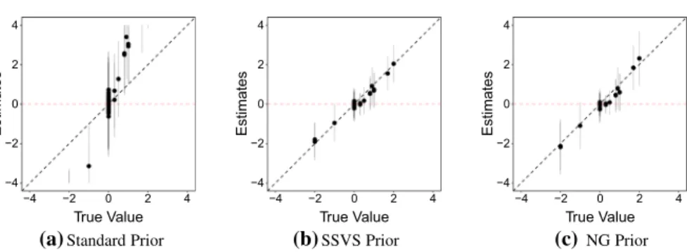
Table1reports the root mean squared error (RMSE) with respect to the coefficients that are truly zero, the coefficients that are truly different from zero, all coefficients and the predicted probabilities (P.P., defined in Eq.5) resulting from the estimation. This enables us to separately examine how well the priors are able to shrink unimportant coefficients to 0, how precise the point estimates are and whether they are able to give useful estimates of the predicted probabilities. These predicted probabilities are of utter importance in the mixture-of-experts framework, as they will directly influence class membership and therefore all estimated model parameters.
The results suggest that the first simulation using 3000 observations is not a very competitive environment. The likelihood is quite informative, resulting in precise estimates even for the standard setup without introducing shrinkage. Figure1plots the true values against the posterior mean estimates of the respective models. The
−4 −2 0 2 4 −4 −2 0 2 4 True Value Estimates
(a)
Standard Prior−4 −2 0 2 4 −4 −2 0 2 4 True Value Estimates
(b)
SSVS Prior −4 −2 0 2 4 −4 −2 0 2 4 True Value Estimates(c)
NG Prior Fig. 1 Posterior mean estimates versus true values for different model setups (with dashed 45◦line) for N = 3000 −4 −2 0 2 4 −4 −2 0 2 4 True Value Estimates(a)Standard Prior
−4 −2 0 2 4 −4 −2 0 2 4 True Value Estimates (b)SSVS Prior −4 −2 0 2 4 −4 −2 0 2 4 True Value Estimates (c)NG Prior Fig. 2 Posterior mean estimates versus true values for different model setups (with dashed 45◦line) for N = 300
uncertainty surrounding the posterior means is given by an interval of±1.96∗S D
whereS Dis the posterior standard deviation. Scatterplots suggest that all three models are able to revocer the true coefficient values well. Nevertheless, the NG setup performs particularly well and even outperforms the SSVS setup in terms of precision. However, it comes at the cost of a slightly prolonged computation time.
Using just 10% of the observations, estimation becomes more difficult as the data becomes less informative as seen in Fig.2. The point estimates become considerably worse. The standard prior has problems to recover the true values, as the enlarged RMSEs indicate. The NG prior shows slight advantages in terms of shrinkage and in predicting cluster membership probabilities. However, the SSVS setup is able to provide more accurate point estimates and therefore has a slightly lower RMSE with respect to the true non-zero coefficients and regarding the overall coefficient RMSE. Further reducing the number of observations toN =100 leads to inflated coefficient estimates and increasing uncertainty when applying no shrinkage, as depicted in Fig.3. This results in enlarged RMSEs. The performance of the SSVS and NG prior remains rather similar to the case with N = 300, however, the shrinkage priors also show larger uncertainty surrounding the posterior means. The SSVS prior produces better point estimates, but is not as efficient as the NG prior when it comes to shrinking unnecessary coefficients to zero. The NG prior shows a slightly better performance when predicting the class membership probabilities. We would like to note that both
−4 −2 0 2 4 −4 −2 0 2 4 True Value Estimates −4 −2 0 2 4 −4 −2 0 2 4 True Value Estimates −4 −2 0 2 4 −4 −2 0 2 4 True Value Estimates
Standard Prior SSVS Prior NG Prior
(a) (b) (c)
Fig. 3 Posterior mean estimates versus true values for different model setups (with dashed 45◦line) for N = 100
the NG prior and the SSVS prior perform rather well in absolute terms, producing small RMSEs in general.11All coefficient estimates of these simulations are provided in Tables4,5 and6 in AppendixD. The performance of the three priors in a full mixture-of-experts classification setting are discussed in the next subsection.
3.2 Classification exercises
To further examine the performance of the priors, four simulation studies in a full mixture-of-experts framework are conducted. These simulations differ from each other with respect to the degree of overlapping of the clusters, the number of regressors and the complexity of the sparsity structure in the true coefficient vectors.
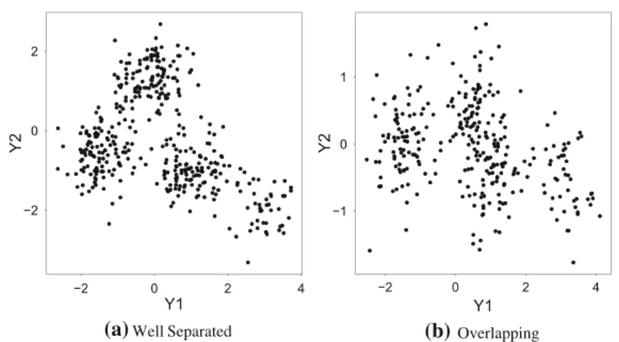
Datasets with 300 observations and four clusters arising from bivariate normal distributions are generated. We differentiate between a “well separated” case and an “overlapping” case usingμ1=(−1.5,−0.5),μ2=(0,1.3),μ3=(1,−1),μ4=
(3,−2)for the “well separated” case andμ1 =(−1.5,0),μ2 =(0.5,0.5),μ3=
(1,−0.5),μ4 = (3,−0.5) for the “overlapping” case, respectively. The variance covariance matricesk are chosen to be 0.25I for the separated case and 0.2I for
the overlapping case for allk = 1, . . . ,4. Figure4 depicts two example datasets, representing the the two cases. In addition, we differentiate between a medium number of regressors (corresponding to the same true coefficient vectors as in Sect.3.1) and a “high sparsity” case where 60 covariates that are not part of the data generating process are added to the covariate dataset, resulting in a total of 80 predictors in the model. Finally, we look at a case with a more complex sparsity structure as compared to Sect. 3.1. In this scenario, the first three predictors are only relevant to the first group, the second three predictors are only relevant to the second group and the third set of four predictors is only relevant to the third group. The last predictor is relevant for all groups. This setup requires the shrinkage priors to flexibly vary the amount of shrinkage by group. An overview of the four different simulation setups is given in Table2.
11 It should also be noted that the performance of the analyzed priors depends on the imposed prior
variances. However, simulations using different variances did not change the results qualitatively. See Frühwirth-Schnatter and Wagner (2011) for a thorough discussion and comparison of various shrinkage priors.
−2 0 2 −2 0 2 4 Y1 Y2 −1 0 1 −2 0 2 4 Y1 Y2
Well Separated Overlapping
(a) (b)
Fig. 4 Example datasets for the “well separated” and “overlapping” simulation scenarios Table 2 Simulation study II overview
Clusters No. of regressors Sparsity structure “Well separated” Separated Medium Simple “Overlapping” Overlapping Medium Simple “High sparsity” Separated Large Simple “Complex sparsity” Separated Medium Complex
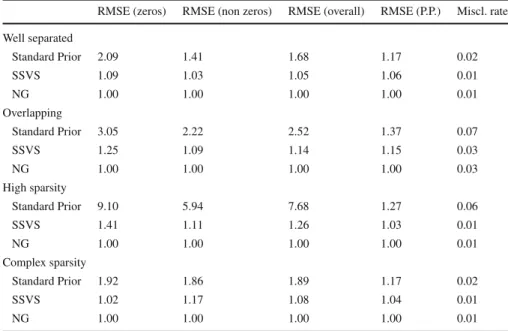
For every setup, various summary statistics are computed. As before, RMSEs with respect to zero and non-zero coefficients as well as overall RMSEs and RMSEs with respect to the predicted probabilities are reported for the models with K = 4. In addition, the misclassification rate of each model is computed. To assess the ability of the models to recover the true number of clusters, we run each simulation study for
K =(2, . . . ,6)and report plots of the average log Bayes factors12with respect to the model with the true number of clustersK =4. Gibbs samplers using 2000 draws after a burn-in period of 5000 draws are implemented. Again, simulations are repeated 25 times and the resulting means of computed statistics across simulations are reported. Table3 reports the main simulation study results. On average, we find that the performance of the SSVS and NG prior is very similar in all simulation exercises. However, a slightly better performance of the NG prior can be found in some cases, especially in the high sparsity setting. Nevertheless, as mentioned before, RMSEs are small for SSVS and NG in absolute terms, suggesting both priors are in principal useful when selecting covariates in a mixture-of-experts framework. We do not report the estimation results forμk andk as all three models perform extremely well in
this regard, showing very similar results. The only issue that stands out is that model with the standard prior has a tendency to overestimate the variances. As pointed out by one of the reviewers, it might be illuminating to look at RMSEs that are separately computed by groups. This does not lead to any significant qualitative or quantitative
Table 3 Simulation study II results
RMSE (zeros) RMSE (non zeros) RMSE (overall) RMSE (P.P.) Miscl. rate Well separated Standard Prior 2.09 1.41 1.68 1.17 0.02 SSVS 1.09 1.03 1.05 1.06 0.01 NG 1.00 1.00 1.00 1.00 0.01 Overlapping Standard Prior 3.05 2.22 2.52 1.37 0.07 SSVS 1.25 1.09 1.14 1.15 0.03 NG 1.00 1.00 1.00 1.00 0.03 High sparsity Standard Prior 9.10 5.94 7.68 1.27 0.06 SSVS 1.41 1.11 1.26 1.03 0.01 NG 1.00 1.00 1.00 1.00 0.01 Complex sparsity Standard Prior 1.92 1.86 1.89 1.17 0.02 SSVS 1.02 1.17 1.08 1.04 0.01 NG 1.00 1.00 1.00 1.00 0.01
The estimates correspond to the average value across 25 runs. RMSEs are reported relative to NG RMSEs
variation in the results. Thus, RMSEs by group are not reported for brevity reasons. More detailed results are available from the author upon request.
Figures5,6,7and8plot the average log Bayes factors relative to the true model with
K =4 for the three priors. Positive values suggest that the respective model scored a higher marginal likelihood than the true model withK =4 and vice versa. In most cases, this model selection criterion suggests to chooseK =4, with two exceptions: First, SSVS seems to have a slight tendency to favor models with a smaller number of clusters as compared to the other models. This leads to positive log Bayes factors for the models withK =2 andK =3 in the “Overlapping” simulation setup. Second, in the “High Sparsity” scenario, all log Bayes factors lean towards models withK =2 andK =3, suggesting influence of the number of predictors on the bridge sampling estimates. However, an in-depth examination of this issue is out of scope of this article and thus left for future research.
All in all, we conclude that the NG prior is a very useful alternative to SSVS in mixture-of-experts frameworks. Generally speaking, the results of the SSVS prior and the NG prior will be very similar, although there are some performance gains of the NG prior visible in terms of shrinkage as well as with respect to model selection issues.
4 HIV information sources in Mozambique
Mozambique is a country in Southeastern Africa that is considered one of the poorest and most underdeveloped countries in the world, scoring low in both economic and
−120 −90 −60 −30 0 2 3 5 6 A v er age Ba y e s F a ctor Standard Prior −150 −100 −50 0 2 3 5 6 A v er age Ba y e s F a ctor SSVS Prior −100 −50 0 2 3 5 6 A v er age Ba y e s F a ctor NG Prior (a) (b) (c)
Fig. 5 Average Log Bayes Factors for different model setups (with dashed line at 0) for well separated case. Reference Model isK=4 −150 −100 −50 0 2 3 5 6 A v er age Ba y e s F a ctor Standard Prior −200 −150 −100 −50 0 2 3 5 6 A v er age Ba y e s F a ctor SSVS Prior −200 −150 −100 −50 0 2 3 5 6 A v er age Ba y e s F a ctor NG Prior (a) (b) (c)
Fig. 6 Average Log Bayes Factors for different model setups (with dashed line at 0) for overlapping case. Reference Model isK=4 −250 0 250 2 3 5 6 A v er age Ba y e s F a ctor −600 −400 −200 0 200 2 3 5 6 A v er age Ba y e s F a ctor −400 −200 0 2 3 5 6 A v er age Ba y e s F a ctor
Standard Prior SSVS Prior NG Prior
(a) (b) (c)
Fig. 7 Average Log Bayes Factors for different model setups (with dashed line at 0) for high sparsity case. Reference Model isK=4
human development rankings. In the year 2008, Mozambique had the 8th highest HIV prevalence in the world with 1,600,000 people infected (11.6% of the population) of whom around 990,000 were women and children. According to the Joint United Nations Programme on HIV/AIDS, there are around 590,000 HIV orphans living in Mozambique, 180,000 of whom are infected with the virus themselves, a large part due to mother-child transmission. 75% of the infected population between the age of 15 and 19 is female. Moreover, a large gender disparity regarding the level of information on the disease can be observed. While around half of the male adolescent
−100 −50 0 2 3 5 6 A v er age Ba y e s F a ctor −150 −100 −50 0 2 3 5 6 A v er age Ba y e s F a ctor −150 −100 −50 0 2 3 5 6 A v er age Ba y e s F a ctor
Standard Prior SSVS Prior NG Prior
(a) (b) (c)
Fig. 8 Average Log Bayes Factors for different model setups (with dashed line at 0) for complex sparsity case. Reference Model isK=4
population has comprehensive knowledge on HIV, only 27.4% of adolescent women have enough information to adjust their behaviour to protect themselves and their children according to the United Nations Children’s Fund. This disparity is suspected to be largely due to socioeconomic and sociocultural reasons, with the main drivers being traditional gender roles and religious involvement (Agadjanian2005).
Consequently, it is crucial to isolate channels that can be used by the government and non-governmental organizations to disseminate vital information on HIV, especially to the female population. Informing females about HIV has proven not only to decrease the infection rate but also increase the economic and social independence of women (Audet et al.2010). Our empirical example contributes to this relevant and important issue by clustering women in Mozambique into groups that are relatively homogenous with respect to their information sources on HIV, similar to Dias (2010). In addition, we use a large dataset of potential geographic and socioeconomic explanatory variables and isolate the most important factors that determine membership in those information clusters. The results may be used to derive for instance information campaign strategies for respective subgroups.
4.1 Bayesian inference for mixtures of Bernoulli distributions
We use a set of binary variables that indicates whether a particular woman uses a specific source to gather information on HIV or not. A convenient choice of mix-ture distribution is the Bernoulli distribution, which proves useful when clustering binary vectors (see for example the vast literature on market segmentation; Wedel and Kamakura2012).
Letyi =(yi,1, . . . ,yi,J)be a J-dimensional vector of 0s and 1s that describe the
HIV information sources used by womani =1, . . . ,N. Assume that this vector is the realization of a binary multivariate random variableY =(Y1, . . . ,YJ). Now suppose
there existKgroups in the population that cause differences in occurence probabilities
γk,j =Pr(Yj =1|Si =k)inK different classes for J different binary variables.Si
is the latent class indicator of womani. We can rewrite Eq.1where yi follows the
f(yi |xi)= K k=1 ηk(xi) J j=1 γyi,j k,j (1−γk,j)1−yi,j. (17)
TheK components correspond to the latent classes in the population. This model is widely used in various research fields, starting as early as Lazarsfeld (1959). For details, see Frühwirth-Schnatter (2006, Ch. 9.5). We assume that all probabilitiesγk,j
are a priori independent and specificy a beta prior of the form
γk,j ∼B(a0,j,b0,j) (18)
and derive the posterior distribution conditional on the latent class indicatorsSi, given
by γk,j|S,y∼B(a0,j+Nk,j,b0,j +Nk−Nk,j) (19) where Nk= N i=1 1(Si =k) Nk,j = N i=1 yi,j1(Si =k). (20) 4.2 Data description
We apply the proposed model to data compiled from the Demographics and Health survey (DHS) for Mozambique from 2003. The DHS is a nationally representative household survey on a wide range of topics, including HIV information sources and various socioeconomic, geographic and health related variables.
The dataset includes information on 11,922 women. Ten different information sources are used to cluster these women into groups and a set of around 40 exter-nal covariates enters the model to explain class membership. These variables cover socioeconomic characteristics like age and education, region of residence, relationship status and sexual behavior as well as poverty related measures and dwelling charac-teristics. Table4provides a detailed overview of the candidate explanatory variables.
4.3 Results
We estimate the model with a NG shrinkage prior for different values of K and compare the resulting models using the marginal likelihood estimates obtained via bridge sampling.13 We choose the model that maximizes the marginal likelihood.
13 The model has been implemented in R (R Development Core Team2008). Computational time for
Table 4 Dataset overview
Description Comments Household level variables
Dwelling characteristics
Household size Number of persons living in household Electricity Household has access to electricity Toilet Household has access to a flush toilet Phone Household has a telephone Bicycle Household has access to a bicycle Motorbike Household has access to a motorbike Car Household has access to a car
Wealth Position in the wealth distribution Dummies for five wealth levels
Geography
Province The province the household is located in. Dummies for the ten provinces of Mozambique Urbanisation Degree of urbanisation Dummy for rural areas Personal level variables
Socioeconomic characteristics
Relationship status Marital status of the women Dummies for married, single, partnership, widowed, living separated and divorced Age Age of the women
Sexual activity Number of sex partners in last 12 months
Religion Religion of the women Dummies for Catholic, Protestant, Muslim, African Zionist, Spiritualist, other and no religion Education Years of schooling
Literacy Classification of the reading ability of the women
Dummies for literate, reading problems and illiterate Employment status Employment status of the
women
Dummy for unemployed HIV information sources
Information source Type of HIV information sources the women use
Dummies for radio, TV, newspapers/magazines, posters, clinic/healthworker, church, school, community meetings, friends/relatives and working place
Fig. 9 Estimates of log marginal likelihoods −36500 −36000 −35500 −35000 2 3 4 5 6 ML Estimate
School TV/Radio Community Modern & Educated
0 1 0 1 0 1 0 1 Church Clinic/Health Worker Community Meetings Friends/Relatives Newspapers / Magacines Poster Radio School TV Working Place Estimated Probability
Fig. 10 Information source estimates for each cluster
The bridge sampling estimates of the log marginal likelihood for K = 2, . . . ,6 are provided in Fig.9. The model with K =4 scores highest and is therefore discussed below.14
The estimates forγk,j are presented in Fig.10. The uncertainty surrounding these
estimates is usually extremely small. At first glance we find that the radio as well as friends and relatives seem to be important information sources for all groups. For the purpose of further interpretation of the model results, we name the groups with respect to their most distinctive HIV information source as described below.
Around 8% of the female population use modern information sources such as television, newspapers and posters. In addition, this group obtains a relatively high amount of information from schools. Thus, we label this group as “Modern & Edu-cated”. A somewhat larger group (around 13% of the population) relies mostly on TV but is highly unlikely to inform themselves in schools. Hence, we name this group
14 This is of course not the only way to proceed here. Especially in a development context, other, more
informal model selection criteria that take into account long term campaigning strategies or financial con-straints may be employed. For example, the groups “Modern & Educated” and “TV/Radio” could be merged as they are both have a distinctive dependence on TV. However, in this paper the statistical possibilities of the proposed model are emphasized and hence we make use of the purely statistical approach.
School TV/Radio Community Modern & Educated −6 −4 −2 0 2 −6 −4 −2 0 2 −6 −4 −2 0 2 −6 −4 −2 0 2 Other Religion Spiritualist African Zionist Protestant CatholicMuslim Maputo Provincia Gaza InhambaneSofala Manica Tete ZambéziaNampula Cabo delgado Niassa Nr. of Sex Partners Yrs. of Educ. Illiterate Problems ReadingRicher Mid Wealth Poor Poorest Unemployed Motorbike Car Bicycle Phone Toilet Electricity Living Separated Divorced Widow Partnership Single Household MembersAge Rural Intercept
Log Odds
Fig. 11 Posterior medians for multinomial logistic regression coefficients (Baseline: “friends/relatives”)
“TV/Radio”. The third group, “School”, which comprises around 6% of the female population of Mozambique, relies heavily on schools for obtaining information on HIV. The baseline group “Community” (73%) has an above average dependence on friends and relatives, community meetings and local churches in terms of information on the disease.
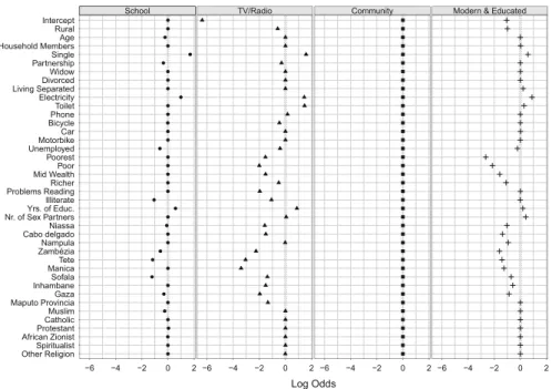
Figure11provides a plot of the point estimates of the logit coefficients.
When interpreting the multinomial logit coefficients, one has to keep in mind that the effects are always interpreted with respect to a baseline group. For convenience in the estimation process, we choose the largest group as baseline group (“Community”). In terms of the other categorical variables, the “baseline woman” is residing in Maputo city, has no religion, is married and is a member of the richest wealth group.
Strong effects of the wealth distribution on the probability of being a member of the “Modern & Educated” and “TV/Radio” group are observable. These groups also share an above average probability of having access to a flush toilet and electricity. In addition, it is relatively unlikely that a woman lives in the countryside and is a member of one of those groups. These findings are in line with what theory suggests in a poverty plagued country like Mozambique.
Unmarried women with above average education are also likely to rely on schools as HIV information sources. This seems puzzling, as female education is a primary development issue in various African countries. However, one should keep in mind that this group is extremely small and comprises just above 6% of the female population. Interestingly, wealth variables seem to be not strongly correlated with the probability of being a member of the “School” group as compared to the other groups. However, we see that geographic variables determine prior class membership for this group,
implying that we can find spatially clustered communities with above average female educational attainment throughout specific provinces.
These results are particularly relevant to policy makers. Important insights that can be derived are, for instance, that HIV information campaigns that are targeted on disseminating educational materials via schools are likely to be more effective in Maputo city as compared to Sofala. It also might be a good idea to target folders that are distributed in schools towards single women as opposed to married women. However, these are mere examples. A detailed discussion of the policy implications of the results is out of scope of this article.
5 Concluding remarks
Finite mixture models are a commonly used tool for model based clustering and den-sity estimation. They can be extended to mixture-of-experts models, allowing to use information from several covariates when clustering dependent variables of arbitrary form. We propose the usage of continous shrinkage priors to find robust predictors of class membership in this context. This enables us to simultaneously identify under-yling groups in a population, cluster said observations into these groups and find the important predictors of being a group member. In particular, we suggest a combination of the normal gamma prior (Griffin and Brown2010) and the Pólya-Gamma sampler (Polson et al.2013) for implicit variable selection in a multinomial logistic regression that is used to model prior class membership.
This setup solves the issue of model uncertainty that arises in this context and reduces the sensitivity of the model with respect to included variables. The proposed framework slightly outperforms related approaches and makes more precise clustering in setups with a large number of predictor variables possible.
We illustrate the model in a real data application where we apply the model with a mixture of Bernoulli distributions to HIV information sources of women in Mozam-bique. Model selection is based on the bridge sampling estimate of the marginal likelihood. We find four clusters of women who are relatively homogenous with respect to their HIV information sources. Somewhat unsurprising, we find that wealth plays an important role in the access to information on HIV. Moreover, geographical patterns of information seeking behavior seem to be prevalent.
Further research may be pointed into the direction of comparing the perfor-mance of different shrinkage priors in this context in a more detailed way as seen in Frühwirth-Schnatter and Wagner (2011). One promising candidate is for exam-ple the Dirichlet–Laplace prior from Bhattacharya et al. (2015). It might also be possible to extend various other Bayesian variable selection methods to mixture-of-experts frameworks, for example Bayesian compression (Guhaniyogi and Dunson
2015) or its extension using targeted random projections (Mukhopadhyay and Dunson
2017). Another interesting problem is how to apply the idea of shrinkage introduced through the prior class membership weights (e.g. Malsiner-Walli et al.2016) for model selection purposes into a mixture-of-experts framework. Also, the evaluation of the forecasting performance of the model was not attempted in this article and is left for further research.
Acknowledgements Open access funding provided by Vienna University of Economics and Business (WU).
Open Access This article is distributed under the terms of the Creative Commons Attribution 4.0 Interna-tional License (http://creativecommons.org/licenses/by/4.0/), which permits unrestricted use, distribution, and reproduction in any medium, provided you give appropriate credit to the original author(s) and the source, provide a link to the Creative Commons license, and indicate if changes were made.
A Choice of hyperparameters & Priors
To enable estimation, it is necessary to choose values for various (hyper-)parameters appearing in the model setup. We setc0=c1=0.01 to obtain a rather uninformative prior distribution as for instance seen in Huber and Feldkircher (2017). However, the only choice of parameter that influences inference is in fact the choice ofθ. Using values close to zero induces rather heavy shrinkage whereas higher values correspond to significantly less shrinkage. As the motivation of the empirical example is to isolate robust determinants of class membership and not to find precise point estimates, we setθto the comparably small value of 0.05 and take the risk of overshrinking some parameters. We set θ to 0.1 in the simulation study. A thorough discussion of the choice and influence ofθcan be found in Bitto and Frühwirth-Schnatter (2018).
B Bridge sampling in mixture-of-experts models
A first step in computing the bridge sampling estimate for the proposed model is to construct an importance density that approximates the modes of the posterior density. As the posterior density of a mixture model will have multiple modes, this problem turns out to be challenging. As one of the proposed model’s benefits is that all posterior distributions are available in closed form, we can make use of the unsupervised impor-tance density construction that has been suggested by Frühwirth-Schnatter (1995) and extended by Frühwirth-Schnatter (2004). The idea is to choose a random subsample ofSposterior densities from theMavailable permutated MCMC draws and use them to automatically construct the importance density. As we use random permutation sampling, this importance density will be multimodal as well.
In practical terms, it is necessary to save the posterior distribution parameters ofS
randomly selected MCMC draws during the sampling process. Note that this implies that the Ssaved parameters of the posterior distributions are not part of the ex post identification procedure. If one has chosen a suitable number of importance densities
Sand number of draws from the importance densityL, we can proceed and draw from the importance density. The idea is to draw from a uniform mixture of S posterior densities. We implement this step as follows. Forl=1, . . . ,L:
1. Choose a random index out of the 1, . . . ,Ssaved posterior density parameters. 2. Fork=1, . . . ,K, generate one draw from the posterior densities with the
param-eters that have been randomly chosen in the previous step. Iterate this procedure. The obtainedMMCMC draws andLimportance density draws can be used in the recursive iteration scheme that has been described in Sect.2.4.
1. Evaluate the importance density draws in the prior densities. 2. Evaluate the importance density draws in the importance density. 3. Evaluate the mixture likelihood using the importance density draws. 4. Evaluate the MCMC draws in the prior densities.
5. Evaluate the MCMC draws in the importance density. 6. Evaluate the mixture likelihood using the MCMC draws.
For a detailed and more formal description for this procedure, see Frühwirth-Schnatter (2004) and Celeux et al. (2018).
C Numerical stability of bridge sampling estimate
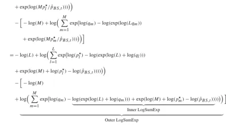
Depending on the sample sizeN, the number of MCMC drawsMand both the number of densities chosen to construct the importance densitySand the number of importance density drawsL, the vectors and matrices that result from evaluating the likelihoods will be large. Hence, the evaluated log-likelihoods may be small in absolute values (e.g.−0.1), but summing over a large number of log likelihoods and exponentiating this sum is prone to numerical underflow. Therefore, we suggest a specific evaluation scheme that has proved numerically stable in our computations. It is based on the idea that we can rewrite the log of the bridge sampling estimate of the marginal likelihood as a double log sum of exponentials. Then we can exploit the following identity:
log i exi =max(xi)+log i exi−max(xi) .
This LogSumExp function can be used to generate an exact and numerically stable estimate of the logarithm of the sum of exponential terms. To employ this function in the bridge sampling procedure, we rewrite the equation of the bridge sampling estimate as follows. log ˆ pB S,t+1 =log L−1lL=1 p l Lql+M p l/pBSˆ ,t M−1M m=1Lqm+M pqmm/pBSˆ ,t = −log(L)+log L l=1 explog( p l Lql+M pl/pˆB S,t) −−log(M)+log M m=1 explog( qm Lqm+M pm/pˆB S,t) = −log(L)+log L l=1
explog(pl)−log(Lql+M pl/pˆB S,t) −−log(M)+log M m=1 explog(qm) −log(Lqm+M pm/pˆB S,t) = −log(L)+log L l=1
+exp(log(M pl/pˆB S,t)))
−−log(M)+log
M m=1
explog(qm)−log(exp(log(Lqm))
+exp(log(M pm/pˆB S,t)))
= −log(L)+log
L l=1
explog(pl)−log(exp(log(L)+log(ql)))
+exp(log(M)+log(pl)−log(pˆB S,t))))
−−log(M)
+log
M m=1
explog(qm)−log(exp(log(L)+log(qm)))+exp(log(M)+log(pm)−log(pˆB S,t))
Inner LogSumExp )) Outer LogSumExp
where the evaluated log likelihoods and the LogSumExp function defined above can be used to generate estimates of the logarithm of the marginal likelihood that are reasonably robust to numeric under- and overflow.
D Simulation study results
See Tables5,6and7.
Table 5 Simulation study results forN=3000
Parameter True Standard prior SSVS Normal gamma
Est. SE Est. SE Est. SE
Group 1 β1,1 0.80 0.82 0.08 0.77 0.08 0.76 0.08 β1,2 1.00 1.02 0.08 0.99 0.07 0.98 0.07 β1,3 2.00 2.04 0.10 2.00 0.09 1.99 0.09 β1,4 0.50 0.53 0.08 0.52 0.07 0.51 0.07 β1,5 0.00 −0.01 0.08 0.00 0.06 −0.01 0.05 β1,6 0.00 −0.01 0.08 −0.01 0.06 0.00 0.04 β1,7 0.00 −0.01 0.08 0.00 0.06 0.00 0.05 β1,8 0.00 0.00 0.07 0.00 0.06 0.00 0.04 β1,9 0.00 −0.02 0.07 −0.01 0.06 0.00 0.04 β1,10 0.00 0.03 0.07 0.02 0.06 0.01 0.04 β1,11 0.00 0.02 0.07 0.01 0.06 0.00 0.04 β1,12 0.00 0.00 0.07 0.00 0.06 0.00 0.04 β1,13 0.00 0.00 0.07 0.00 0.06 0.00 0.04
Table 5 continued
Parameter True Standard prior SSVS Normal gamma
Est. SE Est. SE Est. SE
β1,14 0.00 0.00 0.07 0.00 0.06 0.00 0.03 β1,15 0.00 0.01 0.07 0.01 0.06 0.00 0.04 β1,16 0.00 0.01 0.07 0.00 0.06 0.00 0.04 β1,17 0.00 −0.02 0.07 −0.01 0.06 −0.01 0.04 β1,18 0.00 0.02 0.07 0.01 0.06 0.01 0.04 β1,19 0.00 0.01 0.07 0.01 0.06 0.01 0.04 β1,20 0.00 −0.04 0.07 −0.03 0.06 −0.02 0.04 Group 2 β2,1 0.30 0.28 0.08 0.22 0.08 0.21 0.09 β2,2 0.00 0.00 0.08 0.00 0.06 0.00 0.05 β2,3 0.00 −0.03 0.10 −0.02 0.08 −0.01 0.06 β2,4 0.00 0.00 0.08 0.00 0.06 0.00 0.04 β2,5 −1.00 −1.02 0.08 −1.00 0.08 −0.99 0.07 β2,6 1.70 1.73 0.09 1.69 0.08 1.69 0.08 β2,7 −2.00 −2.06 0.10 −2.01 0.09 −2.00 0.08 β2,8 0.00 0.00 0.08 0.00 0.06 0.00 0.04 β2,9 0.00 −0.02 0.08 −0.01 0.06 0.00 0.03 β2,10 0.00 −0.01 0.08 −0.01 0.06 −0.01 0.04 β2,11 0.00 0.00 0.08 0.00 0.06 −0.01 0.04 β2,12 0.00 0.01 0.08 0.01 0.06 0.00 0.03 β2,13 0.00 0.02 0.08 0.02 0.06 0.01 0.04 β2,14 0.00 0.01 0.08 0.01 0.06 0.01 0.04 β2,15 0.00 0.00 0.08 0.00 0.06 0.00 0.04 β2,16 0.00 0.01 0.08 0.00 0.06 0.00 0.04 β2,17 0.00 0.00 0.08 0.00 0.06 0.00 0.04 β2,18 0.00 0.01 0.08 0.01 0.06 0.00 0.04 β2,19 0.00 0.01 0.08 0.00 0.06 0.00 0.04 β2,20 0.00 0.00 0.08 0.00 0.06 0.01 0.04 Group 3 β3,1 0.30 0.30 0.07 0.24 0.08 0.24 0.08 β3,2 1.00 1.04 0.08 1.02 0.08 1.01 0.07 β3,3 −2.00 −2.06 0.11 −2.01 0.10 −1.99 0.09 β3,4 0.80 0.82 0.08 0.80 0.07 0.79 0.07 β3,5 0.90 0.94 0.08 0.92 0.08 0.91 0.07 β3,6 0.00 0.00 0.08 0.00 0.06 0.00 0.04 β3,7 0.00 −0.03 0.08 −0.02 0.06 −0.01 0.04 β3,8 0.00 0.01 0.07 0.01 0.06 0.01 0.03 β3,9 0.00 −0.03 0.07 −0.01 0.06 0.00 0.04
Table 5 continued
Parameter True Standard prior SSVS Normal gamma Est. SE Est. SE Est. SE β3,10 0.00 0.00 0.07 0.00 0.06 0.00 0.04 β3,11 0.00 0.03 0.07 0.02 0.06 0.01 0.05 β3,12 0.00 −0.01 0.07 −0.01 0.06 −0.01 0.04 β3,13 0.00 0.01 0.07 0.01 0.06 0.00 0.04 β3,14 0.00 0.00 0.07 0.00 0.06 0.00 0.04 β3,15 0.00 0.03 0.07 0.02 0.06 0.01 0.04 β3,16 0.00 0.01 0.07 0.00 0.06 0.00 0.04 β3,17 0.00 0.00 0.07 0.00 0.06 0.00 0.04 β3,18 0.00 0.01 0.07 0.00 0.06 0.00 0.04 β3,19 0.00 0.00 0.07 0.00 0.06 0.00 0.04 β3,20 0.00 0.00 0.07 0.00 0.06 0.00 0.04 RMSE (zeroes) − 6.16 3.94 2.16 RMSE (nonzeroes) − 8.83 8.35 8.35 RMSE (overall) − 6.69 4.94 3.92 RMSE (predicted probabilities) − 3.60 2.94 2.29 Time in sec. − 448.56 449.60 461.41
The estimates correspond to the mean of the posterior means across 25 runs. RMSEs are multiplied by a factor of 100
Table 6 Simulation study results forN=300
Parameter True Standard prior SSVS Normal gamma
Est. SE Est. SE Est. SE
Group 1 β1,1 0.80 1.08 0.30 0.60 0.24 0.52 0.23 β1,2 1.00 1.42 0.33 0.99 0.25 0.92 0.27 β1,3 2.00 2.66 0.42 1.96 0.29 1.97 0.30 β1,4 0.50 0.66 0.29 0.35 0.23 0.28 0.21 β1,5 0.00 0.04 0.32 0.01 0.19 −0.01 0.16 β1,6 0.00 0.01 0.31 −0.03 0.16 −0.01 0.13 β1,7 0.00 0.06 0.32 0.02 0.17 0.00 0.13 β1,8 0.00 −0.06 0.29 0.00 0.14 0.00 0.11 β1,9 0.00 −0.01 0.29 −0.01 0.15 −0.01 0.12 β1,10 0.00 0.06 0.29 0.03 0.15 0.02 0.12 β1,11 0.00 0.00 0.30 −0.01 0.15 −0.01 0.11 β1,12 0.00 0.00 0.29 −0.01 0.16 −0.01 0.13 β1,13 0.00 −0.06 0.29 0.00 0.16 0.00 0.13 β1,14 0.00 0.03 0.29 0.02 0.14 0.01 0.11