Location-aware Associated Data Placement for
Geo-distributed Data-intensive Applications
Boyang Yu and Jianping Pan
University of Victoria, Victoria, BC, Canada
Abstract—Data-intensive applications need to address the problem of how to properly place the set of data items to distributed storage nodes. Traditional techniques use the hashing method to achieve the load balance among nodes such as those in Hadoop and Cassandra, but they do not work efficiently for the requests reading multiple data items in one transaction, especially when the source locations of requests are also distributed. Recent works proposed the managed data placement schemes for online social networks, but have a limited scope of applications due to their focuses. We propose an associated data placement (ADP) scheme, which improves the co-location of associated data and the localized data serving while ensuring the balance between nodes. In ADP, we employ the hypergraph partitioning technique to efficiently partition the set of data items and place them to the distributed nodes, and we also take replicas and incremental adjustment into considerations. Through extensive experiments with both synthesized and trace-based datasets, we evaluate the performance of ADP and demonstrate its effectiveness.
I. INTRODUCTION
Recent Internet developments encourage the emerging of data-intensive applications [1], which leads to a large amount of data stored in the geographically distributed datacenters across regions and a high frequency of data access from the clients or users [2]. Each data request from the users can be fulfilled only at the datacenter holding the requested data or its replicas, so the storage location of the data items really matters to the user-experienced performance. Meanwhile, the optimized data placement can help the service providers by lowering their cost with the improved system efficiency and ensuring the high system availability. Thus we face a general problem of how to efficiently place the data items and replicas to the distributed datacenters, with the requests for them varying across different regions.
Storing the requested data closer to the users is the moti-vation of most existing work on data placement, which helps to reduce the latency experienced by the users and lower the relaying traffic among datacenters. In the network applications that can utilize geographically distributed datacenters, Content Distribution Network (CDN) [3] is broadly applied to help the access of videos, pictures and texts. Different from traditional CDNs where each content is replicated to every datacenter, people need to constrain the number of replicas allowed for each data item under the increasing scale of data items and data traffic. That leads to the problem of how to choose the proper datacenters to store the replicas with a limited number. The issue of multi-get hole [4] has not been paid enough attention to until recently, but it can also affect the decision in placing data items to distributed locations. The issue is
triggered when multiple items are requested in one transaction. People discovered that using fewer nodes to fulfill such a request is better in terms of the system efficiency, because the request dispatched to each node will introduce a certain over-head to the node regardless of the amount of data requested. To overcome the issue, a favorable paradigm is to place the strongly associated data items, those who are often requested together in the same transaction, at the same location. It has profound applications to Online Transaction Processing systems, where a transaction is fulfilled only after accessing multiple data tables, to Online Social Network (OSN) services, where the polling of news feeds involves not only the data of a user itself but also that of its friends, and even to regular web services, since visiting a webpage actually needs to download multiple files, such as the hypertexts, images and scripts.
The balance of the workload or stored items among dis-tributed datacenters is another factor important to the data placement. The maximum serving capacity in a modern data-center seems to be unlimited to an individual service provider, especially when designed as a public cloud. However, a poor balance between datacenters would result in the excessive dependence on some critical locations, which increases the worst-case recovery time after a site failure, and therefore should be avoided as much as possible. Here we only consider the balance among the number of data items (or replicas) placed in different datacenters, but it can partially reflect the balance of workload because of the law of large numbers, assuming the randomness of request rates.
It is challenging to solve a data placement problem that combines these different aspects. We will address the cor-responding issues progressively from three scenarios. First, for the scenario without replicas, we address the placement problem by the hypergraph partitioning formulation, through which the optimized solution can be obtained. Second, we consider thescenario with replicaswhere a certain number of replicas are allowed for each item. The existence of multiple replicas in different locations introduces the decision problem of routing a request, because any one of the corresponding replicas can be used to fulfill the request. A round-robin scheme that iteratively makes the routing decision and replica placement decision is proposed. Third, we consider that the workload may change after a certain time, which makes the earlier solution sub-optimal. Then the problem of replica migration is formulated, i.e., how to change the locations of no more than K replicas based on the existing placement to achieve a better performance. To solve the problem, we
discuss how to generate the candidates for replica migration and determine the optimal number of selected candidates.
The state-of-the-art implementation in most distributed stor-age systems today, such as HDFS [5] and Cassandra [6], is mainly hash-based which can be intuitively understood as random placement. Among the related work that discussed the managed data placement, some existing work either just focused on the distance between data and user, such as [7] and [8], or only addressed the co-location of associated data items, such as [9]–[11]. Some others discussed the issues under the scenario of OSN [12]–[14], where the discussed association of stored entities is only based on pairs of users (each pair consists of a user and one of its friends), which overlooks the relationship between concrete data items as well as the association that involves more than two entities. [15] is the work most related to ours in the problem definition, but it relaxed the group association to pairwise in an early stage of the solution. To the best of our knowledge, our data placement scheme makes the advancement of jointly improving the co-location of associated data and localized data serving without a relaxation of the original objective. Besides, the developed methods to support replicas and to address replica migration are also novel and make the scheme more comprehensive.
The rest of this paper is structured as follows. Section II summarizes some related work. Section III presents our modeling framework for the data placement problem. In Sec-tion V, the locaSec-tion-aware associated data placement scheme is proposed. In Section VI, the scheme is evaluated through extensive experiments. Section VII concludes the paper.
II. RELATEDWORK
Due to the availability of geo-distributed datacenters, there exist multiple choices in selecting the location to store data or the destination to fulfill user requests. In [15], Agarwal et al. presented the automatic data placement across geo-distributed datacenters, which iteratively moves a data item closer to both clients and the other data items that it communicates with. In [16], the replica placement in distributed locations was discussed with the QoS considerations. In [7], Rochman et al. discussed how to place the contents or resources to distributed regions in order to serve more requests locally for a lower cost. In [8], Xu et al. solved the workload management problem, in order to maximize the total utility of serving requests minus the cost, which is achieved through the reasonable request mapping and response routing.
Besides fulfilling the request at a location near to the user, there are other factors that affect the system performance, such as the multi-get hole effect, firstly cited in [4]. The effect can be intuitively explained as follows: for a request to obtain multiple items which are stored distributedly, we favor to use fewer nodes to fulfill the request for a higher system efficiency. It incurs the problem of how to co-locate the strongly correlated data items through the managed data placement. [9] proposed to create more replicas of data items to increase the chance of serving more requested items in one node. [10] mentioned that frequent request patterns can be
discovered through trace analysis, and each group of items frequently accessed can be treated as a whole in the distributed storage. [17] discussed how to co-locate the related file blocks in the Hadoop file system. [11] improved the hypergraph partitioning by compression to more efficiently partition the data items into sets. Such work did not consider the necessity of fulfilling the request locally and was not aware of the difference among locations, which result in that many requests might need to be served at a remote node inefficiently.
Recent research has studied the data and replica placement in OSN, which favors to place data items from close friends together. In [12], Pujol et al. showed the necessity to co-locate the data of a user and its friends and proposed the dynamic placement scheme. In [13], it was stated that different data items from the same user may be requested with a heterogeneous rate or pattern, and the method to determine the proper number of replicas for each data item was given. In [14], Jiao et al. summarized the relationships of entities in the OSN system and proposed the multi-objective data placement scheme. The friendship-based one-to-one data relationship discussed in these works can be considered as a special case of the multi-data association in our modeling.
III. MODELINGFRAMEWORK A. Data Items and Nodes
1 2 3 4 5 (a) (b) 4 5 1 4 1 2 3
Datacenters Request patterns Data item Request pattern Request rateRpy
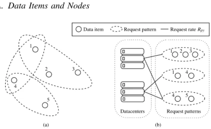
Fig. 1. Problem inputs: (a) request pattern setP; (b) request rate setR
A setXofmdata itemsis used to represent the data stored in the system. Depending on the actual type of data storage, the data items can be files, tables or segments in practice. Users of the service may request at most d different items from the set X in each transaction. We denote the space of
request patternsbyP={X,∅}d. The requests in a practical
system actually fall in a subset of the space, denoted by P ⊂P={X,∅}d . (1)
As illustrated in Fig. 1a, the example system contains 5 different data items and 3 request patterns, which are(1,2,3),
(1,4) and (4,5). The paradigm of accessing multiple data items in one transaction has many applications. For example, the news feed updating in OSN involves the data of multiple users. In data analysis systems, the output is made through combining or processing multiple data files, each captured from a different data source, possibly remotely distributed.
We consider the scenario that the data items are stored in geographically distributed datacenters, represented by a set Y of n nodes. Compared with the centralized storage, the distributed storage can improve the access latency of most users and achieve a higher level of fault tolerance. We term a datacenter as a node or a location interchangeably in the following. Initially, we consider each data item x ∈ X is stored at a unique location y ∈Y. Thus the data-to-location mapping function is defined as
D:x→y , (2)
which specifies the storage locationy of each itemx. Funda-mentally, our work focuses on designing the placement scheme that provides a reasonable solution of D. Besides, we useDy
to represent the set of data items stored in node y.
In the state-of-the-art implementation of such a function, the hash-based methods are adopted most broadly, such as in HDFS and Cassandra, since at the time of their design, the main concern was to achieve the load balance between nodes. Although some other policies take effect in their data placement, such as to avoid placing the replicas of a data item in the same datacenter in order to improve the fault tolerance, the schemes can still be understood as random placement. Obviously the hash-based schemes did not pay enough atten-tion to the system performance affected by the data locaatten-tions and ignored the potential performance improvement through the managed data placement. To attack this deficiency, we start with modeling the metrics of placing data at different locations and the effect of introducing data replicas, and then propose the efficient data placement scheme that fully exploits the benefits of the managed data placement.
B. Data Placement Problem
1) Workload: We assume the request from a client is directed to the datacenter closest to the location of the client. The client can be located outside or inside the datacenters for data storage. When a human user is using the service, they are always from outside locations. Another case is the running jobs or processes inside the datacenter who also can request data items. Without loss of generality, we consider the datacenter that a request is initially accessed to as the source location of the request. So the datacenter or node in our modeling has two roles simultaneously: thesource location of requestsand the destination location holding the stored data.
The workload or request rate of each patternp∈P from the requesting nodey∈Y can be measured, denoted byRpy. We
use the predicted request rates as the input of our scheme to make the data placement decision. There exist mature methods in predicting the rates from a series of rate measurements in the previous time slots, such as EWMA [18], so the details of dealing with prediction are not included in this paper. Although the predicated rates are not the same as the measured ones, we use the same notations in the following for simplicity. First we denote theworkload or request rateset as
R={Rpy|p∈P, y∈Y} . (3)
In the example of Fig. 1b, the request rate setRis illustrated as a bipartite graph, where datacenters and request patterns are the two sets of vertices, and the edges between these two sets are weighted by the rateRpy. Besides, for each data item
x, we calculate its total request rate at each nodey by Rxy=
X
p∈P
Rpy1(x∈p), (4)
where1(x∈p)indicates whether the data itemxis a member of the patternp, returning 1 if true or 0 otherwise. For each pattern p, we calculate its total request rate by
Rp=
X
y∈Y
Rpy . (5)
2) Metrics: Data placement can affect the system perfor-mance in both the system efficiency and user-experienced la-tency. We investigate the relationships between the placement and system performance and summarize them as two metrics. Co-location of Associated Data: The system efficiency is characterized by the necessary system time to fulfill the given workload. According to the observation of [4], in distributed systems, the average system time of a request is not only related to amount of information accessed, but also related to the number of distributed nodes involved due to the processing overhead at each node. Denote the span of a requestpbySp,
representing the number of items requested by it, and denote the number of items in request p that are fulfilled at node y bySpy, since a single node may not be able to provide all
the items inp. They have the relationship ofP
y∈Y Spy =Sp.
Note thatSpyis a variable determined by the mapping function
DandSp is a constant. We model the necessary system time
to partially or fully fulfill a requestpat node y as
Spy+λ·1(Spy), (6)
where the 0-1 function 1(Spy) indicates whether Spy ≥ 1.
The idea behind it is that the system time consists of the part proportional to Spy and the constant overhead of handling
the request, denoted by λ. The latter is introduced by the routine operations in handling a request, such as the TCP connection establishment. With the request rates of different patterns, the total system time of fulfilling all the requests is P p∈PRp P y∈Y[Spy+λ·1(Spy)], which is equal to X y∈Y X p∈P Rp[Spy+λ·1(Spy)] . (7)
Minimizing (7) helps to lower the cost of the service provider, i.e., the amount of resource allocation or the monetary expense on clouds. It can be achieved by the co-location of strongly associated data. For example, in the extreme case, when placing all the items in a pattern pto the same location, the system time on pis at the lower bound Rp(Sp+λ).
BecauseP
y∈Y
P
p∈PRp·Spy in (7) is a constant for any
given workload, we can summarize the metric as CA=X
y∈Y
X
p∈P
Localized Data Serving: The location difference between the requesting node and the node holding the requested data affects the system performance through incurring the relay-ing traffic and enlargrelay-ing the user-experienced latency. To be specific, when the data serving node is not the same as the requesting node, the relaying traffic is introduced, so we use the total relaying traffic as the second metric, denoted by
CL =X
x∈X
X
y∈Y
Rxy·[1−1(x∈Dy)] , (9)
where 1(x ∈ Dy) indicates whether x is stored at node y.
Here we use the relaying traffic as the metric of localized data serving, but it is still possible to use thelogical distance
between each user and its requested data as the metric instead, which is not included in the paper due to the page limit.
Note that [14] summarized the relationships in the data placement for OSN as two categories: (a) between data and data; (b) between data and node. Our work is different at (a), as we consider each request may involve a group of multiple data. We cannot adapt to their scheme through simply decomposing the multi-data relationship to the pairwise relationships of all the pairs in the group. Due to the generalized hypegraph formulation shown later, our scheme can be extended to incorporate most of the metrics considered in that paper.
3) Optimization Problem: Our objective is to improve the performance of a placementD, represented by
C(D) =CA+αCL , (10) whereαis used to tradeoff the two metrics above. To minimize C(D) helps to improve the system efficiency and the user-experienced latency. Besides, the balance among nodes is also necessary. To ensure the worst-case recovery time upon site failure, the number of data items stored in different datacenters should be balanced. Therefore, we set the balance constraint
that the number of items stored in each datacenter y, should be in a range [(1−)ha,(1 +)ha], whereha is the average
number of items in all nodes and is the balance parameter. The formulated problem can be generalized as: given I = {P, R}, find the optimal placement solution ofD:x→y that minimizes the value ofC(D), subject to the balance constraint.
C. Data Replicas
The data placement problem is more challenging if the replicas of data items are allowed. We would not differentiate the data item itself and its replicas, so both of them are treated as replicas below. The allowed number of replicas for each item is given from a separate process not discussed here, due to the scope of this paper. Below we assume the number of replicas for each data item is k, but the scheme still applies when the number is heterogenous for different items. Because the locations of replicas need to be determined, the data-to-location mapping function is updated to
D:x→ {y1, y2, ..., yk}. (11)
Meanwhile, we have to face the routing decision problem, since the request for an itemxcan be fulfilled at any location
Data−node edge 1 2 3 4 5 A B Data item Node Hyperedge Set Vertex Set
Request pattern edge
Fig. 2. Hypergraph formulation
holding a replica ofx. We adopt the deterministic routing and represent the routing as a mapping function
M: (x, p, y)→yd , (12)
which can give the routing destination yd ∈Y for each item
xin a patternprequested from nodey. Note that the solution for the scenario with replicas should include bothDandM. Besides, we realize that the routing decision should be made based on a given placement of replicas, however after the decision is made, the previously generated placement might be sub-optimal. This makes the problem more complicated and we will present our solution gradually in the following.
IV. ASSOCIATEDDATAPLACEMENT A. Placement without Replicas
We start with showing that without data replicas, the opti-mization problem can be formulated as ann-way hypergraph partitioning problem. Note that in the existing work that also used hypergraph to model to the relationship among multiple items, e.g., [11], the exact data location was not addressed because of their unawareness of the difference between loca-tions. A hypergraph G(V, E)is a further generalization of a graph, i.e., the hypergraph allows each of its hyperedges to involve multiples vertices while the edge of an ordinary graph can only involve two vertices at most. In our scheme, we set up the vertex set V with all the data items and all the nodes in the considered system, such as
V ={X, Y} . (13)
The hyperedge setE contains all the request patterns and the pairs between each node and each data item. For each request pattern hyperedge, it involves multiple data items and that is the main reason of introducing hypergraph. Formally,
E=n{ep|p∈P},{exy|x∈X, y∈Y}
o
. (14) Each hyperedge e ∈ E is assigned a weight. Due to the objective (10), the weights are set according to
we=
(
λRp, for the request pattern hyperedgeep
αRxy, for the data-node hyperedgeexy
. (15) An example of formulating the problem into a weighted hypergraph is illustrated in Fig. 2. In the hypergraph, there are two types of vertices: storage node (square) and data item (circle), and two types of edges, the request pattern hyperedge
(dashed circle) and the data-node hyperedge (solid line). We may term hyperedge as edge for short below.
An n-way partitioning of the hypergraph is to partition its vertices intonoutput sets, such that each vertex only belongs to one of the n sets. The cut weight of the partitioning is counted as the sum of the cut weights of its hyperedges. A hyperedge e is cut if its vertices fall to more than one sets; thecut weight of edgeeis counted as(t−1)weif its vertices
fall to t sets. Meanwhile we can pre-assign some vertices to the noutput sets before applying the hypergraph partitioning algorithm, i.e., they are fixed-location vertices. In our scheme, each of thennodes is pre-assigned to a different set before the partitioning. By that, after the partitioning, we obtain where to place a data directly from the noutput sets, because each node and the data items stored in it would fall to the same set. Next we show the equivalence between the cut weight of an n-way hypergraph partitioning and the objective value C(D)
of the data placement based on the partitioning result.
Theorem 1: For any inputI, we can formulate it into a hy-pergraph through the method above. Partition the hyhy-pergraph into n sets of vertices, from which, we can obtain the data placement D. Denoting the cut weight of the partitioning by H, it satisfies that H =C(D)−B, where B is a constant.
Proof: First, we discuss the cut weight of a request pattern edge ep, denoted by Hp. According to the definition
of the cut of hyperedges, Hp = [Py∈Y 1(Spy)−1]wep = [P
y∈Y 1(Spy) − 1]λRp. With (8), We can obtain CA −
P
p∈PHp =Pp∈PλRp =B, which is a constant. Second,
we discuss the cut weight of a data-node edge exy, denoted
by Hxy. For any data item x, it was connected to all the
nodes in the formulated hypergraph. After the partitioning, it can be connected to only one node, because otherwise some sets in the partitioning result would be connected by x, considering that we have assigned each node to a different set. Assuming the item xis finally connected with node fx,
the sum of the cut weights of data-node edges related toxis P
y∈Y Hxy = Py∈Y /fxαRxy. After placing the data items
according to the partitioning, with (9), we obtain the metric CL = P x∈X P y∈Y /fxRxy. Therefore, H = P p∈PHp+ P x∈X P y∈Y Hxy =C A−B+αCL=C(D)−B.
From the thereom, to minimize the cut weight of the hy-pergraph partitioning is the same as to minimize the objective function (10). The minimum n-way hypergraph partitioning has been shown to be NP-Hard, but different heuristics have been developed to solve the problem approximately, because of the wide applications of the hypergraph partitioning, such as in VLSI, data mining and bioinformatics. The PaToH tool [19] is what we use to partition the formulated hypergraph.
The general steps of the algorithm in PaToH [19] are as follows: 1) coarsen the initial hypergraph into smaller and smaller scales gradually; 2) solve the partitioning problem on the smallest scale graph; 3) gradually uncoarsen the partitions into the larger scale graph with refinements. The coarsening process may eliminate the chance of placing some vertices in the same set, but with a reasonable coarsening and later refinement, its performance can be still quite well.
B. Placement with Replicas
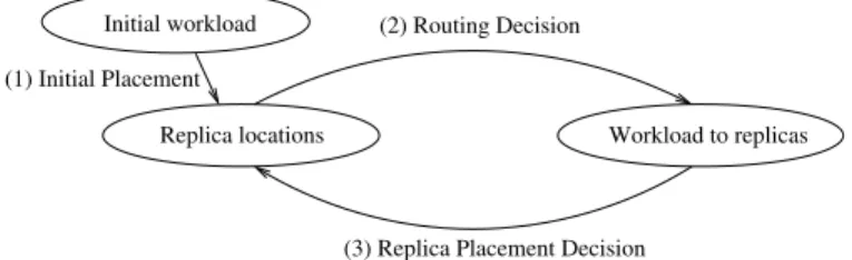
To overcome the issues introduced by the replicas, we design the round-robin scheme as shown in Fig. 3. In phase (1), we address the initial placement of data replicas by a simple greedy method. In phase (2), the local routing decision is made for each request pattern from each node, considering the existence of replicas. Then the request patternpattached with each request rateRpy is refined towards specific replicas. In
phase (3), based on the refined request rates towards replicas, we can make the replica placement decision. Phase (2) and (3) are applied repeatedly until the improvement is smaller than a threshold. The general steps of the whole scheme are shown in Alg. 1. Details of each phase are given as follows.
Initial workload (1) Initial Placement
(2) Routing Decision
(3) Replica Placement Decision
Workload to replicas Replica locations
Fig. 3. Logic flow of the scheme with replicas
1) Initial Placement: First we present a greedy method of generating the initial replica placement, which is illustrated as phase (1) in Fig. 3. For each datax∈X, we obtain the set Wx={Rxy|y ∈Y}, representing the request rates to datax
from different locations, and sort it to the descending order. Based on the allowed number of replicas for datax, which isk in our model, we chooseknodes that are with the highest rate inWx to store the replicas of item x. This initial placement
at least ensures that the resultant total relaying traffic of the system is minimized, which is better than a random initial placement. Although the metric of data co-location is not considered in this phase, the final performance of the scheme is not affected, since that metric takes effect in the later steps.
2) Routing Decision: A main problem introduced by al-lowing replicas is to make the optimal routing decision based on the current status of the replica placement, which is shown as phase (2) in Fig. 3. We formulate the optimization problem for the routing of patternpat nodej as follows.
min λX y∈Y Ay+α X x∈p X y∈Y /j Xxy s.t. X y∈Y Xxy·1(x∈Dy) = 1,∀x∈p Xxy≤Ay, Xxy∈ {0,1}, Ay∈ {0,1},∀x∈p (16)
The optimal solution of (16) ensures the minimized value of (10) under any given replica placement. The binary variable Xxy is used to represent whether an itemx∈pwill be routed
to the node y. And the binary variable Ay indicates whether
the node y is utilized (or active) in the routing of p. The constraints ensure that each item x ∈ p is actually routed to one node holding the replica of x and being active. The objective is to minimize the cost incurred by the fulfillment
of request p from node j. Its first part is about the number of nodes involved. The second part is the relaying traffic in fulfillingp. Indeed they would contribute to the objective (10). We can generalize a feasible solution to (16) as two cases: the local node j is or is not included in the chosen active data serving nodes. For the former, we prefer to choose any itemx∈pto be served locally if possible, because otherwise, moving the serving to the other locations would introduce the extra relaying traffic. The latter is still necessary, because if we assume that all the items are not served at the local node j, it saves the cost of λAj compared with the former, which
may be able to compensate for the extra relaying traffic. No matter either case is chosen, the amount of relaying traffic would be determined, and then the objective becomes λP
y∈Y Ay, which makes the problem to the classical
set-cover problem. The set-set-cover problem is proved to be NP-hard, however we can use any Integer Linear Programming solver or heuristics to obtain the approximate solution. In our method, we obtain the solution of two cases first and then choose the one with a lower objective value for (16). For the former case, we choose data items to be served locally as much as possible and then apply the set-cover heuristic to the remaining items. For the latter, we directly apply the set-cover heuristic to all the data items. The heuristic is to iteratively choose the node that covers the highest number of data items not covered yet by the nodes chosen in the earlier iterations.
3) Placement Decision: The placement decision is obtained through extending the solution for the case without replicas. We denote the set of replicas byZ and denote a replica byz. After phase (2), because the routing decisionMis obtained, we can determine the request rate to each replica. We refine the workload set from R={Rpy} toR0={Rp0y}, which is
shown asF uncRin Alg. 1. The difference betweenpandp0is that p0 is based on the replica space. Formally,p0 ∈ {Z,∅}d.
Specifically, pcan only indicate whether a data item x is in the pattern p, but p0 indicates which specific replica of each
itemx∈pis actually involved in fulfilling the request. Then in phase (3), with the obtained workload on the replica space, we make the replica placement decision through extending the hypergraph formulation. The vertices in the hypergraph become the union of the replica set and node set. In the edge set, the data-node edges are substituted by the replica-node edges. The weights of edges are set according to
we=
(
λRp0, for the request pattern edgeep0
αRzy, for the replica-node edgeezy
. (17) Based on the above formulation, we can still apply the hyper-graph partitioning algorithm as in the scheme without replica. The time complexity of the n-way hypergraph partitioning algorithm is O (|V|+|E|) logn
, so the time complexity of our scheme is no more than O (|P|+km)nlogn
.
After applying the hypergraph partitioning, we obtain the replica placement result, which in fact is the input of making routing decision in the next round. After rounds of iterations of the routing decision and placement decision, the obtained
Algorithm 1 Associated Data Placement with Replicas
1: D ←P hase1(I) .Initial replica placement
2: C←0
3: repeat
4: M ←P hase2(D) .Routing decision
5: R0 ←F uncR(M,I) . Obtain workload to replicas
6: I0← {R0, P} .Inputs on the replica space
7: D ←P hase3(I0) .Hypergraph partitioning
8: Clast ←C
9: C←C(M,D) 10: untilC−Clast < γ
11: return M,D
performance tends to keep stable, and we would stop the iteration after the improvement is less than a threshold γ. Finally, the placement and routing decision in the last round are informed to the nodes in the system. With the deterministic routing decisionM, we can obtain a hash mapping function for each node, whose input is a request pattern and output is the routing destination of each item in the pattern. Such a function ensures the dispatch of any requests can be made in a very short time which is important for a practical system.
C. Replica Migration
When the workload changes, it is not necessary to adjust the system through completely overriding the existing data place-ment. Therefore we formulate the replica migration problem and propose the incremental adjustment method. In a practical system, we are given a budget of changing the locations of data replicas. So in the formulatedreplica migration problem, we try to minimize the objective (10) through changing the locations of no more than K replicas, based on the exiting placement solutionD, under the changed workload.
Consider that there are N replicas in total, we can set N −K of them as fixed-location vertices in the hypergraph formulation, just as we pre-assigned each node to a set previously, and then continue the iterative process above to determine the locations of the remainingK replicas, who are chosen as candidates of replica migration. Then the problem is how to choose the K candidates. Our idea is to select those replicas whose location change can potentially provide a higher gain to the system performance. The strategy in the choosing theKcandidates is given as follows. For each replica z of data itemxthat previously located at nodej, we define the gain of its migration as
gz= max j0∈Y /j
gz,jA →j0+α·gLz,j→j0} , (18)
which is the maximum benefit after moving it to any other location j0. In (18), gA
z,j→j0 and gz,jL →j0 correspond to the
two metrics in the modeling. For the former, we calculate the benefit of moving replicaz fromj toj0, from the perspective of co-locating associated data. Note that the location change of z would affect related request patterns. Representing the benefit in terms of the number of nodes used to fulfill a request
since the moving by the function∆jpy→j0, we define gAz,j→j0=−λ X p∈P 1(x∈p)X y∈Y Rpy∆j→j 0 py . (19)
For the latter, we define it as the maximum relaying traffic decrease at the new location j0 deducting the traffic increase at the old location j, such as
gLz,j→j0 = (1−1(x∈Dj0))Rxj0−Rzj . (20)
After sorting the migration gaingzof all the replicas in the
system, the replica with a higher gain is preferred to be moved away from the original location. Meanwhile, we realize that more thanKcandidates can be chosen at the beginning, but it may result in more thanKreplicas with location changed after the hypergraph partitioning. So a binary search is applied to find the optimal candidate number that yields a solution with at most K replicas being migrated finally.
Algorithm 2 Replica Migration
1: Zc← ∅;G← ∅;Nt←N;Nb←K
2: forz∈Z do . Obtain migration gain of replicas
3: G← {G, gz}
4: end for
5: whileNt6=Nb do .Binary search in [K, N]
6: Nc ←(Nt+Nb)/2
7: Zc ←ChooseNc replicas as candidates based onG
8: M0,D0← Apply Alg. 1 with{Z−Z
c} being fixed
9: Nm←Location changes betweenD0 and original D
10: IfNm> K,Nt←Nc; otherwise, Nb←Nc
11: end while
12: returnthe bestM0,D0 ensuring N
m≤K
The pseudo-code of replica migration is shown in Alg. 2. We obtain the set G containing the migration gain of all replicas through line 2–4. The iteration of binary search is executed in line 5–11. In each iteration, Nc is the number
of selected candidates before hypergraph partitioning and the replicas with a higher gain in the sorted G are selected as candidates, denoted by Zc. The replicas not included in Zc
are marked as fixed in applying the hypergraph partitioning. Nm is the number of replicas actually migrated, obtained by
comparing the new placement and the old one. The binary search ensures that Nmin the solution can get close toK.
V. PERFORMANCEEVALUATION A. Experiment Settings
We have implemented the proposed scheme and conducted several studies. In the experiments, we consider there aren= 10datacenters (or nodes), which are geo-distributed. The total number of data items ism= 10,000. The number of request patterns in the system is |P| = 40,000. In the simulation, for each request pattern, the data items involved are generated first, by randomly selecting at mostd= 40items from the set of mitems. Previous studies, e.g., [20], have shown that in a broad range of network services, the request rates to different
contents follow the Zipf distribution [21]. So the request rate for each pattern is generated following the Zipf distribution with indexH = 0.8. After that, a node is uniformly generated, set as the source location of that request pattern. The default values of other parameters are λ= 5.0,α= 1.0 and= 0.1, considering the general small-size data item storing scenario. Besides the proposed schemeADP, the other schemes imple-mented and being compared with include:Hash,Closest,
Multigetand their variants to fit the case in which replicas
are allowed. Hash places the data items to the nodes based on the hashing results, representing the state-of-the-art imple-mentation.Closestplaces a data item to the node that has the largest request rate to that particular item. Multiget
optimizes to place the associated data in the same location extremely, but does not consider the localized data serving.
The metrics we used in the evaluation include:
Co-location: We calculate the average number of data serv-ing nodes involved to fulfill each request, which is weighted by the request rate, and then show the result of dividing it by n= 10. It is directly related to the metricCAin the modeling. Localization: We also show the percentage of the data items thatis notserved locally among all the requests. It is directly related the metricCL in the modeling.
Objective: Our optimization objective is given in (10), which is the weighted sum of CA and CL. The objective value
shown in the figures is normalized with regard to the obtained objective value ofHashunder the same settings by default.
Balance: We also evaluate the balance of each scheme. Denoting the number of replicas in nodes byh1, ..., hn, it is
calculated bymaxn
i=1|hi−ha|/ha, whereha=P n i=1hi/n.
B. Experiment Results
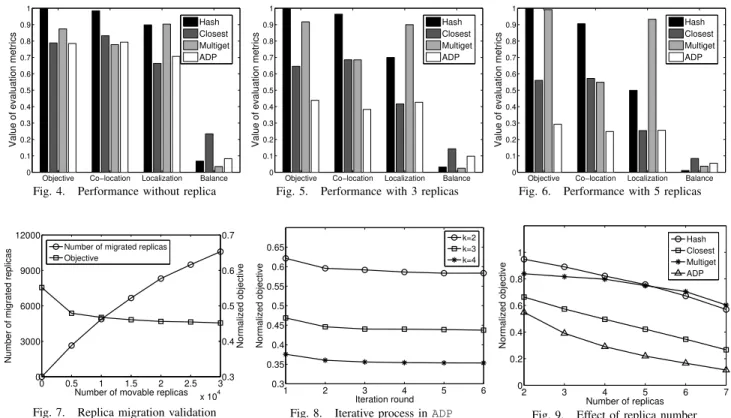
1) Scenario without Replicas: In the first experiment, we study the performance ofADPand compared schemes in a no-replica scenario. Fig. 4 compares the metrics obtained based on their placement results. We can observe thatADPperforms the best on the objective and the gap betweenHashand other three schemes is apparent. In terms of co-location,Multiget
achieves the best performance, because it focuses on the associated relationship among data items in the placement.
Closestachieves the best performance on localization, since
in its design, each data item is always placed to the node with the largest request rate to it. However,Multiget and
Closest only consider one of the two aspects.
Compar-atively, by optimizing both aspects in a unified way, ADP
achieves the lowest objective value even if its performance is not the best on either individual metric. Here the shown improvement through ADP is not significant because of the conflict between the two metrics and the limited optimization space without replicas. We also compare the balance result of different schemes. Although it is shown that the balance of
ADPdegrades when compared withHash, the balance is still in the acceptable range. According to the results ofADP, the maximum and minimum number of items in each of the 10 nodes is1,083and937respectively, while the average number of items in each node is1,000.
Objective Co−location Localization Balance 0 0.1 0.2 0.3 0.4 0.5 0.6 0.7 0.8 0.9 1
Value of evaluation metrics
Hash Closest Multiget ADP
Fig. 4. Performance without replica
Objective Co−location Localization Balance
0 0.1 0.2 0.3 0.4 0.5 0.6 0.7 0.8 0.9 1
Value of evaluation metrics
Hash Closest Multiget ADP
Fig. 5. Performance with 3 replicas
Objective Co−location Localization Balance
0 0.1 0.2 0.3 0.4 0.5 0.6 0.7 0.8 0.9 1
Value of evaluation metrics
Hash Closest Multiget ADP
Fig. 6. Performance with 5 replicas
0 0.5 1 1.5 2 2.5 3 x 10⁴ 0 3000 6000 9000 12000
Number of movable replicas
Number of migrated replicas
0.3 0.4 0.5 0.6 0.7 Normalized objective
Number of migrated replicas Objective
Fig. 7. Replica migration validation
1 2 3 4 5 6 0.3 0.35 0.4 0.45 0.5 0.55 0.6 0.65 Iteration round Normalized objective k=2 k=3 k=4
Fig. 8. Iterative process inADP
2 3 4 5 6 7 0 0.2 0.4 0.6 0.8 1 Number of replicas Normalized objective Hash Closest Multiget ADP
Fig. 9. Effect of replica number
2) Scenario with Replicas: We further evaluate the perfor-mance of different schemes under the scenario with replicas. When the replica number is 3, the objective value of ADP
outperforms the others by more than 20%, as shown in Fig. 5. It achieves the near-optimal performance on the localized data serving and gives the best performance on the co-location of associated data, by exploiting the existence of replicas. When the replica number is increased to5, the performance of
ADP is even better, as shown in Fig. 6, such as the objective improvement is more than 90% when compared with other schemes. As for the balance, the node difference on the number of stored replicas is still not large in all the schemes. In fact, when compared with Closest, which more relies on the uniform workload from different locations to achieve the balance, in ADP, we can initiatively control the result of balance through adjusting the balance parameter of the hypergraph partitioning algorithm, which will be shown later.
3) Replica Migration: We simulate the workload change by randomly shuffling the request rates of all request patterns. The replica migration method is validated as follows: arbitrarily set the number of movable replicas before applying the placement algorithm, denoted by Nc; then after applying the algorithm,
obtain the number of replicas changing location, denoted by Nm, and the objective value. We set the replica number to
3, resulting in 30,000 replicas in total. Then we change Nc
from 0 to 30,000 in the experiment, where 0 indicates the performance without any migration and 30,000 indicates the performance of a complete overriding of the exiting placement. As shown in Fig. 7, the increase of Nc enlarges the scope of
movable replicas, which yields the decrease of the objective value. WhenNc = 5,000, more than50% of the replicas are
actually migrated and the objective value shows the largest decrease, which validate the effectiveness of our candidate selection. The monotonically increase ofNmwith the increase
of Nc validates that the binary search is applicable here.
4) Others: To further investigate the performance of ADP
and validate its effectiveness in design, we take extra experi-ments. Fig. 8 plots the change of the objective value in rounds of iterations in Alg. 1. We expect that the solution is improved through repeatedly making the routing and replica placement decision. As shown in the figure, after about 3–4 rounds, the objective value tends to keep stable. Besides, the method is effective to different numbers of replicas.
To show the effect of changing the number of replicas, we plot Fig. 9. The shown values are all normalized towards the objective value ofHashwithout replica, to show the trend of performance change under the same scheme. When the number of replicas is increased, the system performance is expected to be improved, such as more requests can be satisfied locally or through fewer nodes. In the figure, ADP shows a better performance in all the cases tested. In practice, the number of replicas cannot be too large as it increases the storage cost of the system and the difficulty of consistency maintenance.
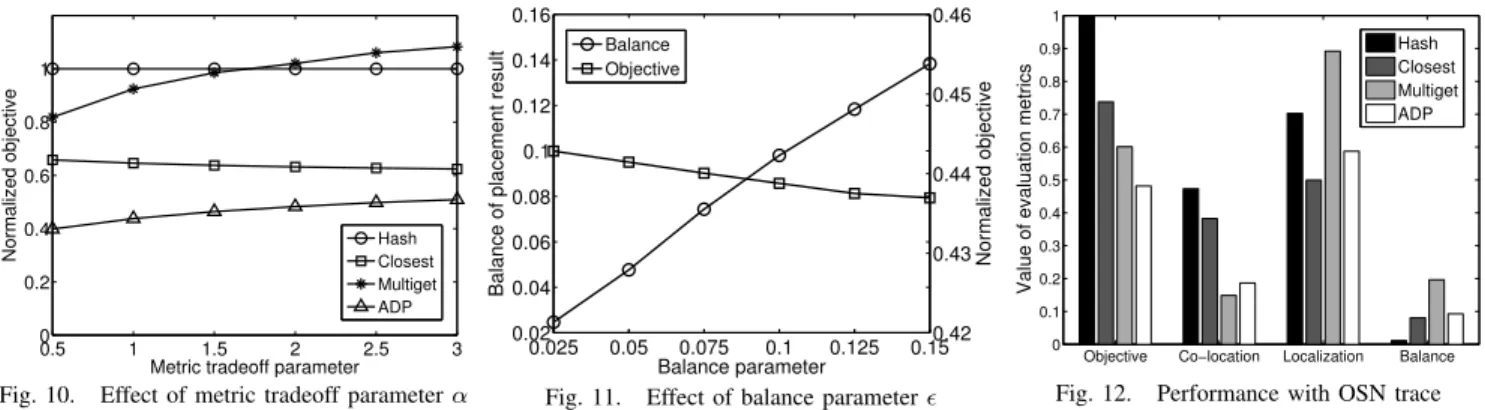
The parameter α in (10) can tradeoff the importance of the data co-location and localized data serving. We change its value, and show the corresponding objective value in Fig. 10. When α is larger, the improvement of ADP over
Closestbecomes less. It is because that the weight of the
localized data serving metric is increased in the objective function and the latter can give the optimal performance on that metric. Meanwhile, the performance ofMultigetgets worse because of not paying attention to that metric.
0.5 1 1.5 2 2.5 3 0 0.2 0.4 0.6 0.8 1
Metric tradeoff parameter
Normalized objective HashClosest
Multiget ADP
Fig. 10. Effect of metric tradeoff parameterα
0.025 0.05 0.075 0.1 0.125 0.15 0.02 0.04 0.06 0.08 0.1 0.12 0.14 0.16 Balance parameter
Balance of placement result
0.42 0.43 0.44 0.45 0.46 Normalized objective Balance Objective
Fig. 11. Effect of balance parameter
Objective Co−location Localization Balance
0 0.1 0.2 0.3 0.4 0.5 0.6 0.7 0.8 0.9 1
Value of evaluation metrics
Hash Closest Multiget ADP
Fig. 12. Performance with OSN trace
The hypergraph partitioning algorithm can take the balance parameter as input, which allows us to flexibly control the balance in ADP. We plot Fig. 11 to compare the results with different as the input of the algorithm. The increase of makes the nodes less balanced but results in a lower objective value. Besides, it is shown that the resultant balance metric is always lower than the input. So inADP, given the acceptable level of balance, we can tune the parameter to improve the system performance while satisfying the balance constraint.
We further make an experiment with an OSN dataset [22]. We extract the friend relationships from the dataset and simu-late the scenario that a user polls the updates of all its friends when using the news feed updating function. We consider each user as a data item, which results in 45,092 data items and 63,102 request patterns in the experiment. The request rates are randomly generated following the Zipf distribution and the source location of each request pattern is also random. On weighted average, each request pattern contains 11.22 items. The number of replicas is set to k = 2. The comparison results are shown in Fig. 12, which also validate the better performance of our proposed scheme. Here the running of
ADPlasts about 292.8 seconds on the Xeon E5645 CPU, and we will further improve the running efficiency in the future.
VI. CONCLUSIONS
We studied the balanced data placement problem for ge-ographically distributed datacenters, with joint considerations of the localized data serving and the co-location of associated data. By formulating the scenario without replicas using a hy-pergraph, we presented the framework to obtain the optimized solution. We further addressed the placement problem under the replica scenario, by introducing the iterative process of routing and replica placement. Besides, the method that mi-grates replicas based on the existing placement was proposed to deal with the workload change. Finally, we evaluated the proposed scheme through extensive experiments.
ACKNOWLEDGMENT
This work is supported in part by NSERC, CFI and BCKDF. REFERENCES
[1] M. Armbrust, A. Fox, R. Griffith, A. D. Joseph, R. Katz, A. Konwinski, G. Lee, D. Patterson, A. Rabkin, I. Stoica et al., “A view of cloud computing,”Communications of the ACM, vol. 53, no. 4, pp. 50–58, 2010.
[2] A. Greenberg, J. Hamilton, D. A. Maltz, and P. Patel, “The cost of a cloud: research problems in data center networks,” ACM SIGCOMM computer communication review, vol. 39, no. 1, pp. 68–73, 2008. [3] M. Rabinovich and O. Spatscheck, Web Caching and Replication.
Addison-Wesley, 2002.
[4] “Memcached Multiget Hole,” http://highscalability.com/blog/2009/10/ 26/facebooks-memcached-multiget-hole-more-machines-more-capacit. html.
[5] “HDFS Architecture Guide,” http://hadoop.apache.org/docs/r1.2.1/hdfs design.html.
[6] “About Replication in Cassandra,” http://www.datastax.com/docs/1.0/ cluster architecture/replication.
[7] Y. Rochman, H. Levy, and E. Brosh, “Resource placement and assign-ment in distributed network topologies,” inProc. of IEEE INFOCOM, 2013.
[8] H. Xu and B. Li, “Joint request mapping and response routing for geo-distributed cloud services,” inProc. of IEEE INFOCOM, 2013. [9] S. Raindel and Y. Birk, “Replicate and bundle (RnB)–a mechanism for
relieving bottlenecks in data centers,” inProc. of IEEE IPDPS, 2013. [10] R. Nishtala, H. Fugal, S. Grimm, M. Kwiatkowski, H. Lee, H. C. Li,
R. McElroy, M. Paleczny, D. Peek, P. Saabet al., “Scaling memcache at Facebook,” inProc. of USENIX NSDI, 2013, pp. 385–398. [11] A. Quamar, K. A. Kumar, and A. Deshpande, “Sword: scalable
workload-aware data placement for transactional workloads,” in Proc. of EDBT, 2013, pp. 430–441.
[12] J. M. Pujol, V. Erramilli, G. Siganos, X. Yang, N. Laoutaris, P. Chhabra, and P. Rodriguez, “The little engine (s) that could: scaling online social networks,” inProc. of ACM SIGCOMM, 2010.
[13] G. Liu, H. Shen, and H. Chandler, “Selective data replication for online social networks with distributed datacenters,” inProc. of IEEE ICNP, 2013.
[14] L. Jiao, J. Li, W. Du, and X. Fu, “Multi-objective data placement for multi-cloud socially aware services,” inProc. of IEEE INFOCOM, 2014. [15] S. Agarwal, J. Dunagan, N. Jain, S. Saroiu, A. Wolman, and H. Bhogan, “Volley: Automated data placement for geo-distributed cloud services,” inProc. of USENIX NSDI, 2010.
[16] X. Tang and J. Xu, “On replica placement for QoS-aware content distribution,” inProc. of IEEE INFOCOM, 2004.
[17] W. Wang, K. Zhu, L. Ying, J. Tan, and L. Zhang, “Map task scheduling in mapreduce with data locality: Throughput and heavy-traffic optimal-ity,” inProc. of IEEE INFOCOM, 2013.
[18] J. S. Hunter, “The exponentially weighted moving average.”Journal of Quality Technology, vol. 18, no. 4, pp. 203–210, 1986.
[19] U. V. Catalyurek and C. Aykanat, “PaToH: Partitioning tool for hyper-graphs,”http:// bmi.osu.edu/ umit/ PaToH/ manual.pdf.
[20] P. Gill, M. Arlitt, Z. Li, and A. Mahanti, “YouTube traffic characteriza-tion: a view from the edge,” inProc. of ACM IMC, 2007, pp. 15–28. [21] L. A. Adamic and B. A. Huberman, “Zipf’s law and the internet,”
Glottometrics, vol. 3, no. 1, pp. 143–150, 2002.
[22] J. Kunegis, “Konect - the koblenz network collection,” in Proc. of Int. Web Observatory Workshop, 2013. http://konect.uni-koblenz.de/ networks/facebook-wosn-links.