Time Varying Volatility and the Cross-Section of Equity Returns  

Time-Varying Volatility and the Cross-section of Equity

Returns

Chris Brooks

ICMA Centre, University of Reading

Xiafei Li

Nottingham University Business School

Joelle Miffre

EDHEC, Nice, France

March 2009

ICMA Centre Discussion Papers in Finance DP2009-01

Copyright 2009 Brooks, Miffre and Li. All rights reserved

.

ICMA Centre •University of Reading

Whiteknights •PO Box 242 • Reading RG6 6BA • UK Tel: +44 (0)1183 787402 • Fax: +44 (0)1189 314741 Web: www.icmacentre.ac.uk

Director: Professor John Board, Chair in Finance

Time-Varying Volatility and the Cross-section of

Equity Returns

Abstract

A vast literature has documented the value premium and the small firm effect as pervasive stylized facts in empirical asset pricing and yet research has been largely unable to provide entirely convincing explanations of why these phenomena exist. This paper demonstrates that the cross-sectional variation in returns between portfolios sorted by size and book-to-market value is significantly and positively related to the conditional volatility of those portfolios. We show that the explanatory power of the portfolios’ sensitivities to conditional volatility for the cross-section of returns is in addition to that embodied in the sensitivities to market risk, macroeconomic, book-to-market and market capitalization factors.

Keywords: cross-sectional variation in stock returns, CAPM, GARCH-M, conditional volatility, risk premium.

JEL classifications: G12, G14

I. Introduction

The Capital Asset Pricing Model (CAPM) of Sharpe (1964) and Lintner (1965) is one of the most important tenets of modern finance. The model predicts that differences in returns are solely driven by differences in systematic risk and that there is a static linear relationship between the two. The success of the model and its ability to sustain criticism is quite enduring given that numerous articles have called its major implications into question. In particular, it is now well-known that differences in returns relate to differences in size and book-to-market (B/M) values (for example, Fama and French, 1992) and that betas are time-dependent (e.g., Bollerslev et al., 1988). Along the same lines, conditional versions of both the CAPM and the consumption CAPM have been shown to perform substantially better than their static counterparts in explaining the cross-sectional variation in expected returns of size- and B/M-sorted portfolios (Jagannathan and Wang, 1996; Lettau and Ludvigson, 2001). Against this wealth of evidence, the failure of the static CAPM to explain the pricing of risky assets seems hard to dispute.

This paper adds to the asset pricing literature by studying the cross-sectional relationship between varying volatility and expected returns. Our measure of time-varying volatility takes into consideration the variance and therefore the idiosyncratic volatility of a portfolio’s returns as described by the generalized autoregressive conditional heteroskedasticity in mean (GARCH(1,1)-M) model of Engle et al. (1987). The rationale for choosing this model is twofold. First, our version of the asset pricing model augmented with a GARCH(1,1)-M specification explicitly deals with the problem of conditional heteroskedasticity that has plagued previous studies of the CAPM. As well as having constant betas, the static CAPM also assumes that the variances of the error terms are constant.

However, numerous researchers have found that for financial time series, the variances of the error terms change over time in a partially predictable fashion (see for example French et al., 1987; and Schwert and Seguin, 1990) and exhibit volatility clustering, where large (small) volatility changes tend to be followed by large (small) volatility changes. Our version of the CAPM augmented with a GARCH(1,1) specification suitably relaxes the assumption of homoscedasticity in the residuals by capturing the impact of new information (as measured by the error term) on the conditional variance of a portfolio’s returns through the most recent squared error. Second, our model augmented with GARCH(1,1)-M terms explicitly treats the conditional volatility of portfolio returns as a way to explain the cross-section of returns by adding to the mean equation of the CAPM a GARCH(1,1)-in-mean term. The essence of the rationale for our approach is that the release of new information (captured by the error term) may cause the risk (conditional variance) of size- and B/M-sorted portfolios to change over time in a way that is priced and can be captured by our augmented model.

We show that cross-sectional differences in average returns directly relate to differences in the total risk of the portfolio returns. Our finding that the return of small and value stocks is related to time-varying idiosyncratic risk in a fashion unrelated to unexpected changes in macroeconomic factors lends support to the idea that the CAPM anomalies based on size and B/M may well relate to a lack of diversification of the size and B/M-sorted portfolios. This result is in line with the notion that agents who fail to fully diversify their portfolios demand higher average returns to compensate them for bearing higher levels of firm-specific risk (Merton, 1987). Our paper therefore indirectly contributes to the debate on

the possible role of unsystematic risk in explaining stock returns.1 An alternative explanation

for our conclusion that conditional volatility is priced relates to a missing risk factor that is proxied by conditional volatility. Further evidence however suggests that the explanatory power of conditional volatility persists even after accounting for the risks embodied in size, B/M, macroeconomic and financial factors. So the missing factor does not seem to be related to the typical sources of risk documented in the asset pricing literature.

The rest of the study is organized as follows. Section II develops a model for expected returns that motivates our findings and that accounts for the cross-sectional explanatory power of time-varying volatility for stock returns. Section II also presents the methodology employed to study the relation between time-varying volatility and average returns. Section III describes the data. Section IV reports the results and finally section V offers some concluding remarks.

II. Methodology

A. Model for Expected Returns

Let us assume that the pricing of most stocks and all portfolios is governed by a two-factor conditional APT model and thus that returns are generated by a process such as

(1) R_Pt =E(R_P)+

β

_PM

(

R_Mt −E

(

R_M

)

)

+

β

_P1

(

F_1t −E

( )

F₁

)

+

υ

_Pt

1

While Ang et al. (2006, 2008) report that stocks with high levels of idiosyncratic risk have low future average returns, Goyal and Santa-Clara (2003), Ghysels et al. (2005), Jiang and Lee (2006), Diavatopoulos et al. (2008) and Fu (2009) found the opposite; namely, a positive relation between idiosyncratic risk and stock market returns. Note also that Bali et al. (2005) and Bali and Cakici (2008) argue that the results of Goyal and Santa-Clara (2003) could be spuriously driven by small, illiquid stocks traded on the Nasdaq and critically depend on the measure of idiosyncratic volatility used, the sample studied and data frequency.

where RPt is the time t return on a portfolio P, RMt is the return on a value-weighted portfolio of all assets present in the economy, E(.) is the expectation operator, F1t is a non-specified risk

factor with zero correlation with RMt,

β

PM (

β

P1) is the sensitivity of portfolio P to the market

portfolio M (risk factor F1) and

υ

Pt is a white-noise error term. Let us apply the no-arbitrage

argument of Ross (1976) to this hypothetical world with two conditional risk factors. In the absence of arbitrage opportunities, the following linear risk-return relationship must hold

(2) E R_{Pt t PM Mt P Ft} 1 1 0 ) ( =λ +β λ +β λ

where λ0t is the time t return on the risk-free asset, λMt =E

(

RMt

)

−Rft is the price of market

risk at time t, _Ft = E

( )

R_Ft −R_ft

1 1

λ is the risk premium associated with F1t and E

( )

RF₁t is the

expected return of a mimicking portfolio that has an unit sensitivity to factor F1t and zero correlation with RMt.

In anticipation of the results in Section IV, the paper shows that time-varying volatility is priced, since it governs a positive risk premium that is significant at the 10% level or better. This result suggests that the conditional CAPM misses a risk factor F1t that mimics

the behavior of the time-varying volatility of the portfolios’ returns. Once this omitted risk factor is explicitly modeled via our GARCH(1,1)-M approach, it explains the cross-sectional pricing of equity returns beyond the explanatory power of other factors such as size, B/M,

macroeconomic shocks and market returns; namely, 0

1t ≠

F

λ in equation (2).

B. Econometric Specification and Tests

The methodology we employ is a variant of the two-step methodology of Fama and MacBeth (1973). The first step follows Engle et al. (1987) and consists of a GARCH(1,1)-in-mean estimation of model (3)

(3)

(

)

1 2 1 − − + + = + + − + = − Pt P Pt P P Pt Pt Pt Ph ft Mt PM P ft Pt h h h R R R R

θ

ε

γ

ω

ε

β

β

α

where RPtare the 100 size- and B/M-sorted portfolios of Fama and French (1992), Rftis the

risk-free rate, RMtis the market return, εPt ~ N

(

0,hPt

)

, hPt is the conditional variance of portfolio P

returns, βPM and βPh are the sensitivities of portfolio P to the market portfolio M and to the

portfolio volatility h_Pt respectively, αP is a constant and ωP, γP, and θP are conditional

variance parameters to estimate. To ensure that hPt is non-negative, non-degenerate and that the GARCH(1,1) process is covariance stationary, requires that the conditions

0

>

P

ω

,0<

γ

_P <1,0≤

θ

_P <1 and

γ

_P +

θ

_P <1 are satisfied. The augmented model with a GARCH(1,1) specification for the conditional variance allows the conditional variance to depend not only on past shocks but also on past realizations of the conditional variance itself. Model (3) also adds to the mean equation a conditional standard deviation term and estimates

βPh, the loading of each size- and B/M-sorted portfolio P on its time-varying volatility hPt .

Model (3) is first estimated over the sample July 1926 to June 1936. While it is standard practice to apply the two-step methodology to size- and B/M-sorted portfolios over 60 consecutive observations, windows of 120 months are used in this study to ensure convergence of the GARCH model optimization routine. For the sake of consistency, the same 120 observations are used to test the CAPM and Fama and French (1992) model.

In a second step, we test whether the observed sensitivities to risk factors (βPM and β Ph) are priced sources of risk. Indeed, while equity returns may be sensitive to conditional

total risk, a necessary condition for this to be a source of priced risk is that investors receive a reward for bearing this risk. The estimates of βPM and β Ph for P (=1, …, 100) are used to

explain the section of mean returns in each month from July 1936 to June 1937. The cross-sectional regression in a given month is as follows

(4) R_i −R_f =λ₀ +λ_Mβ_Mi +λ_hβ_hi +ϑ_i

where the subscript i (=1, …, 100) denotes each of the 100 portfolios in the cross-sectional regression, λM is the price of market risk, λh is the price of volatility risk, λ0 is an intercept and

i

ϑ is an error term. Following Fama and French (1992), a variant of the second step that considers the size and book-to-market value of equity as potential sources of priced risk is also estimated each month

(5) Ri −Rf =λ0 +λMβMi +λMVMVi +λBMBMi +λhβhi +ϑi

where λMV and λBM are the prices of risk associated with the size and book-to-market value of

equity, respectively, MV is the log of the market value of the Fama and French (1992) portfolios measured in June 1936 and BM is the log of the book-to-market value of the Fama and French (1992) portfolios measured in December 1935. This step produces 12 estimates of the vector {λ0,

λM, λMV, λBM, λh}.

Finally, the sample is rolled-over by 12 observations at a time, with each repetition of the two steps producing 12 new estimates of each of the factor risk premia. t-tests are then performed on the resulting risk premia to determine which factors have explanatory power for the cross-section of realized stock returns. For the CAPM to be valid, the hypotheses that

0

=

MV

λ ,

λ

_BM =0 and λ_h =0 should not be rejected and

λ

_M should be positive at conventional levels of statistical significance.

For comparison and completeness, a variant to this general framework that involves a different specification of conditional volatility is also considered. Nelson (1991), Glosten et al. (1993) (hereafter GJR) and Rabemananjara and Zakoian (1993) show that good news (as

measured by positive shocks) and bad news (as measured by negative shocks) may have an asymmetric impact on the conditional variance of stock returns. In particular, it has been shown that volatility is higher for negative returns than positive returns of the same magnitude. This has been argued to arise either from “leverage” (the impact of falling versus rising stock prices on a firm’s debt-to-equity ratio) or “volatility feedback” effects. In equation (6), we explicitly capture this potential asymmetric effect and test whether the returns on size- and B/M-sorted portfolios respond in the same way to good and bad news. As a result, we amend model (3) as follows

(6)

(

)

1 2 1 1 2 1 − − − − + + + = + + − + = − Pt P Pt t P Pt P P Pt Pt Pt Ph ft Mt PM P ft Pt h I h h R R R R

θ

ε

η

ε

γ

ω

ε

β

β

α

ηP measures any asymmetric response of volatility to good and bad news, εPt ~N

(

0,hPt

)

,

1

1 =

− t

I if ε_Pt−1 <0 (bad news) and I_t−1 =0 otherwise. Now, the conditions for non-negative and non-degenerate hPt and covariance stationarity are

ω

P >0,0<

γ

P <1, 0≤

θ

P <1,

γ

P +

0 2

/ ≥

P

η

and

γ

_P +

η

_P /2+

θ

_P <1. We test the cross-sectional pricing of time-varying risk in that framework too by studying the significance of the parameter estimates of (4) and (5).

III. Data and Preliminary Analysis

Our dataset comprises the 100 size- and B/M-sorted portfolios of Fama and French (1992).2 The portfolios include all NYSE, AMEX, and NASDAQ stocks with market values as of December of t-1 and June of t and positive book value of equity for t-1. At the end of June, all stocks are ranked into 10-decile portfolios based on their size, each size decile is then split

2

We are thankful to Kenneth R. French for providing the series on his website: http://mba.tuck. dartmouth.edu/pages/faculty/ken.french/data_library.html.

into 10 B/M-sorted portfolios. The stocks in the portfolios are value-weighted and the positions are held over the following 12 months, when the portfolios are formed again. The full sample period for the 100 size- and B/M-sorted portfolios runs from July 1926 to December 2006 and is split into two sub-periods (pre and post June 1963) for consistency with Fama and French (2006) and Ang and Chen (2007) among others. The value-weighted return on all NYSE, AMEX, and NASDAQ stocks in excess of the one-month Treasury bill rate is used as a proxy for the market risk premium. To test the cross-sectional explanatory power of size and B/M, the average market value and book-to-market value of each portfolio are also downloaded.

Table 1, Panel A presents the reward-to-risk ratios of the 100 size- and B/M-sorted portfolios. To conserve space, the results are reported for the period July 1963 – December 2006 solely. The portfolios with small capitalization and high B/M outperform the portfolios with large market capitalization and low B/M on a risk-adjusted basis. The post-1963 value premium is greater for the portfolios with small market capitalization than for the portfolios with large market capitalization. Similarly, the size effect rises with the B/M value of the portfolios. These results are consistent with Loughran (1997), Daniel and Titman (1997), Davis et al. (2000),Fama and French (1992, 1993, 2006) and Ang and Chen (2007).

[Insert Table 1 around here]

We perform OLS regressions of the excess returns of the 100 size- and B/M-sorted portfolios on a constant and the market excess returns3. If the static CAPM is an adequate characterization of the temporal variation in returns, the variances of the error terms should be constant. This motivates us to perform a series of Lagrange Multiplier (LM) tests to assess the

3

validity of the static CAPM under the null hypothesis that there is no autoregressive conditional heteroskedasticity (ARCH) (Engle, 1982) in the errors. Following previous studies in the time-series literature, we test for ARCH(12)-effects. The test statistic is asymptotically distributed as a χ2 variate with 12 degrees of freedom under the null hypothesis of no ARCH. The results, reported in Table 1, Panel B, clearly indicate that the portfolios over the 1963-2006 period show substantial evidence of ARCH effects: With only 2 exceptions, all of the LM statistics are significant at the 5% level. Therefore, it is perhaps no surprise that previous authors (Fama and French, 1992, 1993, 2006; Ang and Chen, 2007) concluded that the static CAPM fails to explain the post-1963 performance of the 100 Fama and French portfolios. The misspecification of the static CAPM identified in Table 1, Panel B gives us a further incentive to augment the static CAPM with GARCH-M terms as in (3) or with GJR-GARCH-M terms as in (6).

IV. Empirical Results

This section estimates our augmented version of the CAPM that explicitly models time-varying volatility. Subsection A studies the time-series properties of the parameter estimates in (3) and (6) and subsection B analyzes the cross-sectional properties of conditional volatility within the CAPM of Sharpe (1964) and the three-factor model of Fama and French (1992). Finally, Subsection C brings forward some possible reasons for the observed results.

A. The CAPM with a (GJR-)GARCH(1,1)-M Specification: Time-Series Results

The preceding section highlighted the need to allow for heteroskedasticity in the errors of the CAPM models for the post-1963 period. This is done by assuming that the conditional

variances of portfolio returns follow a GARCH(1,1) process. We also add βPh hPt to the

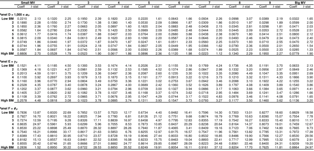
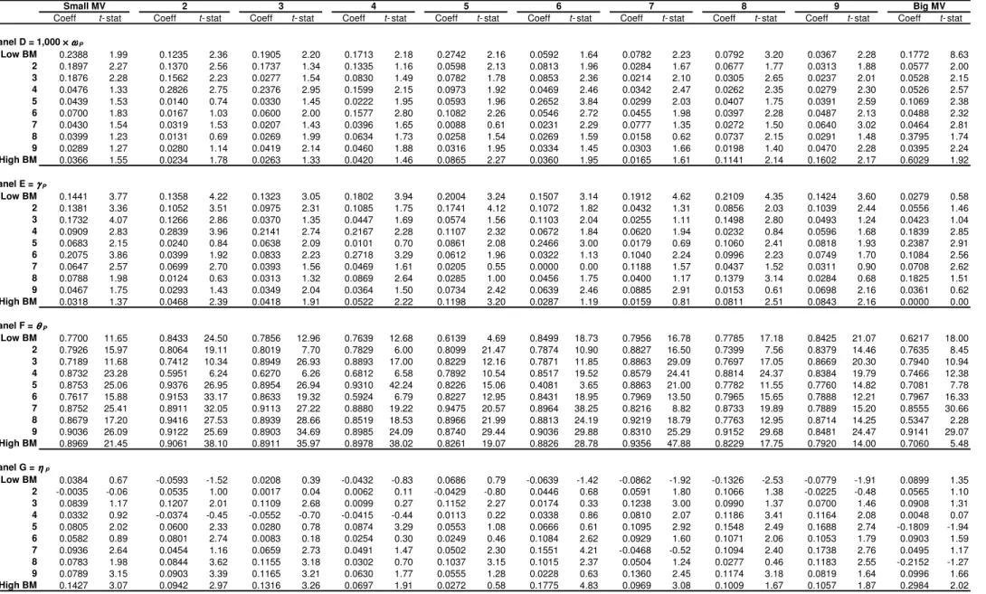
CAPM mean equation and subsequently estimate models (3) and (6). Tables 2 and 3 present the estimates of models (3) and (6), respectively. In each table, Panels A to C (D to G) report the coefficient estimates from the mean (conditional variance) equation.

[Insert Tables 2 and 3 around here]

Panels A of Tables 2 and 3 report the regression intercepts and Panels B of Tables 2 and 3 report the CAPM betas of the 100 portfolios for the specifications without and with the asymmetry term included in the conditional variance model respectively. The dispersion in market betas in Panels B mimics that of MV-sorted mean returns, with the average βPM of the

smallest capitalization portfolios exceeding that of the largest capitalization portfolios by 0.166 (t-statistic of 3.81) in Table 2 and by 0.205 (t-statistic of 6.78) in Table 3. This result is mainly driven by the lowest B/M portfolios for which the fall in market betas from the small MV to the large MV portfolios at 0.354 is particularly noticeable in both tables. However, the dispersion in market betas fails to reproduce that of B/M-sorted mean returns. Indeed, the performance of the highest B/M portfolios exceeds that of the lowest B/M portfolios; yet, the average βPM of the highest B/M portfolios is less than that of the lowest B/M portfolios with a

difference of -0.297 (t-statistic of -5.63) in Table 2 or -0.343 (t-statistic of -11.68) in Table 3. This result is consistent with Fama and French (2006) and Ang and Chen (2007), who show that the static CAPM is unable to account for the post-1963 value premium.

The results in Table 2 Panel C indicate that for a given size, the value portfolios are more sensitive to their conditional total risks than the growth portfolios: the coefficient βPh,

albeit universally insignificant at the 5% level, are indeed higher for the high B/M portfolios (0.0552 on average) and lower for the low B/M portfolios (-0.0353 on average), with a

difference in average βPh of 0.0905 that is significant at the 1% level (t-statistic of 6.04).

Similarly, for a given B/M, the portfolios with small capitalization tend to be more sensitive to their conditional total risks than the portfolios with large capitalization: the coefficient βPh,

albeit insignificant at the 5% level, are indeed higher for the low MV portfolios (0.0467 on average) and lower for the high MV portfolios (0.0041 on average), with a difference in average βPh at 0.0426 that is significant at the 1% level (t-statistics of 2.98). The same

conclusions apply to the results in Table 3, Panel C: The average βPh coefficientof the value

portfolios exceeds that of the growth portfolios by 0.0933 (t-statistic of 6.58) and the average

βPh coefficientof the small MV portfolios exceeds that of the large MV portfolios by 0.0411

(t-statistic of 2.99). Clearly, even though the coefficients βPh are insignificant, conditional

volatility seems to be doing a good job at capturing the dispersion in returns between the portfolios with high and low B/M and between the portfolios with small and large MV.

Panels D to F (G) of Table 2 (3) report coefficient estimates for the conditional variance equation of models (3) and (6). The coefficient estimates are often positive and significant at the 5% level, suggesting that, irrespective of the portfolio under consideration, the (GJR)-GARCH(1,1) specification does capture the time-variation in the total and idiosyncratic risks of the portfolio returns. We split the 100 portfolios into 4 quadrants of 25 portfolios (small-growth, small-value, large-growth and large-value) and calculate the average of the GARCH parameter estimates in each quadrant. γP in Table 2 and γP + 0.5×ηP inTable 3

measure the impact of recent information on volatility. It appears that γP averages 0.14 for the 25 portfolios in the North-West quadrant of Table 2 (small-growth) versus 0.12 for the remaining 75 portfolios. Similarly, γP + 0.5×ηP averages 0.14 for the portfolios in the

that the smaller the MV and the smaller the B/M of a stock, the higher the impact of recent information on the volatility of its returns. The θP coefficient captures the impact of historical

information on volatility. It is equal to an average of 0.82 (0.87) for the 25 portfolios in the small-value quadrant and to an average of 0.79 (0.81) for the remaining 75 portfolios, suggesting that older information has a slightly greater influence on the volatility of the value and small size stocks. Finally, ηP measures the asymmetric impact of bad and good news on

volatility. The average value of the estimated parameter is 0.03 for the portfolios in the small-growth quadrant versus 0.09 for the portfolios in the large-value quadrant. Thus, following the announcement of bad news, volatility rises more for value stocks with large capitalization than it does for growth stocks with small capitalization.

For the results presented in Tables 2 and 3, we also calculate the difference in each of the parameter estimates (averaged across all size deciles) between the extreme value and extreme growth deciles. These mean differences (with t-ratios to test the null hypothesis of no difference between B/M deciles 1 and 10 in parentheses) for the GJR-GARCH-M model (Table 3) parameters are:4 αP: 0.0025 (2.91); βPM: -0.34 (-11.68); βPh: 0.093 (6.58); ωP:

-0.00002 (-0.47); γP: -0.101 (-7.72); θP: 0.089 (3.91); ηP: 0.149 (5.65). It is evident that the

extreme value portfolios have significantly higher exposures to time-varying total volatility and also significantly different volatility dynamics (although their average levels of volatility are not significantly different, emphasizing the inadequacy of unconditional volatility as a potential explanation for the value premium). The extreme value decile portfolios have significantly less spiky variances (lower γP), although their volatility persistence is

4

Results are very similar for the model without asymmetry terms (CAAPM-GARCH-M in Table 2) and hence are not reported.

comparable. Volatility increases significantly more sharply for value stocks than growth stocks following bad news than following good news of the same magnitude.

We then repeat this analysis but this time focusing on the differences in the parameter estimates (averaged across all B/M deciles) between the very smallest and the very largest size sorted portfolios. These mean differences (t-ratios in parentheses) for the GJR-GARCH-M model (Table 3) are: αP: -0.0005 (-0.74); βPM: 0.20 (6.78); βPh: 0.04 (2.99); ωP:

-0.06 (-0.91); γP: 0.0098 (0.30); θP: 0.089 (2.25); ηP: 0.03 (0.67). These results show that the

stocks in the smallest decile have comparable conditional mean intercepts but statistically significantly higher exposures to both market risk (average difference in βPM is 0.20) and total

risk (average difference in βPh is 0.04). Small stocks show more persistence in volatility but

there are no significant differences in the average volatility (ωP), the volatility of volatility

(γP), or the degree of asymmetry (ηP) between the smallest and largest decile portfolios.

B. The CAPM and Fama and French (1992) Model Augmented with (GJR-) GARCH(1,1)-M Terms: Cross-Sectional Results

The preceding section relates the returns of size and B/M-sorted portfolios to their levels of time-varying volatility. A necessary condition for this risk to be priced is that investors receive a significant reward for bearing it; namely, the price of volatility risk has to be significant at conventional statistical levels. Results from these tests are reported in Tables 4 and 5 for the CAPM and Fama and French (1992) model, respectively. The tables present the average parameter estimates across the windows and their associated t-ratios. In each table, Panel A reports the results for the full sample from July 1926 to June 2006 (hereafter 26-06), Panels B and C focus on the two sub-sample periods from July 1926 to June 1963 (hereafter

26-63) and from July 1963 to June 2006 (hereafter 63-06), respectively. The first (second) sub-sample entails the estimation of 324 (522) rolling cross-sectional regressions, while the full sample entails the estimation of a total of 846 regressions.

[Insert Table 4 around here]

The main conclusion from Table 4 is that conditional volatility, as modeled by both the GARCH(1,1)-M and the GJR-GARCH(1,1)-M terms, is priced. The estimates of λh in

equation (4) are indeed positive and significant at the 1% level for the whole sample (Panel A) and for the second sub-sample (Panel C). They are also positive, albeit insignificant, in the first sample (Panel B). When the GARCH(1,1)-M model is used to measured conditional volatility, a 1% increase in βhi in (4) leads to 1.67%, 1.19% and 1.97% increases in monthly returns in

Panels A, B and C, respectively in column (3). Should the GJR-GARCH(1,1)-M specification be used instead (column (4)), a 1% rise in βhi leads to increases in returns of 1.37%, 0.67%

and 1.80% a month over the periods 26-06, 26-63 and 63-06, respectively. There is thus a positive relationship between average returns and βhi. This confirms our hypothesis that stocks

with high B/M and low MV characteristics earn more simply because they are more risky. In sharp contrast, market risk is never priced (the hypothesis that λM = 0 is not rejected at

conventional levels). This conclusion holds irrespective of whether or not conditional volatility is treated as a risk factor.

We also analyze the pricing of conditional volatility without the requirement for the specification of a market portfolio. In this case, the first step of the two-step methodology does not treat the market portfolio as a risk factor and considers only the conditional volatility of the portfolio returns in the mean equation. The second step is simply to regress mean excess returns on a constant and βhi as estimated from the first step. The results reported in

column (5) of Table 4 show that conditional volatility is also priced on its own and commands positive risk premia that range from 2.43% to 3.64% a month over the periods 26-63 and 63-06, respectively. The risk premium associated with conditional volatility is significant at the 1% level over the whole sample and the second sub-sample.

Note, however, that while conditional volatility is priced, the intercept of the cross-sectional regression λ0 remains positive and significant at the 1% level over the periods 26-06

and 63-06. This tells us that even our version of the CAPM augmented with conditional volatility fails to fully capture the cross-sectional variation in equity returns. However, the inclusion of conditional volatility in the CAPM cross-sectional equation (4) seems to consistently reduce the estimate of λ0 (from an average of 0.76% a month in column (2) to

averages of 0.62% and 0.61% in columns (3) and (4), respectively). This indicates that our specification of the model with (GJR)-GARCH(1,1)-M terms does a better job of describing the cross-sectional variation in equity returns than the standard CAPM. Altogether, the results reported in Table 4 confirm the general belief that the CAPM fails to explain the cross-section of equity returns because it embodies the wrong measure of risk.

Table 5 reports parameter estimates from the cross-sectional regression (5). In effect, we now augment the market model with the log of the size and the log of the B/M of the 100 Fama and French (1992) portfolios and analyze the pricing of time-varying volatility within this augmented model. The conclusions of Table 4 on the pricing of conditional volatility are robust to the inclusion of size and B/M. This suggests that volatility risk does not merely proxy for the risks previously measured with size and B/M. The risk premia associated with volatility risk are positive and significant at the 10% level or better over the periods 26-06 and 63-06. They are also positive, albeit insignificant, over the period 26-63. Volatility risk

commands monthly risk premia that range from 0.46% (GJR-GARCH(1,1)-M over the period 26-63) to 0.78% (GJR-GARCH(1,1)-M over the period 63-06). The monthly price of volatility risk equals 0.66% on average in the augmented Fama and French model of Table 5 versus 1.52% in the augmented CAPM of Table 4. While it represents only 43% of the corresponding figure in Table 4, the price of volatility risk in Table 5 is still significant in both economic and statistical terms. Conditional volatility risk is also priced when market beta is omitted and size and B/M only are considered as risk factors. As reported in column (5) of Panel A (Table 5), the price of volatility risk at 1.65% a month is then comparatively higher than in columns (3) and (4) (0.65% and 0.66% a month respectively).

[Insert Table 5 around here]

The results of Table 5 confirm the conclusions of Table 4 with respect to the failure of the CAPM to explain the cross-section of equity returns. Not only is the price of beta risk (λM) insignificant throughout all samples and models, but also two factors related to B/M and

conditional volatility are priced. In spite of the predictions of the CAPM to the contrary, cross-sectional differences in stock returns are not related to cross-sectional differences in market betas. Differences in average returns relate in a positive way to differences in the B/M value of equity and to differences in conditional volatility: the higher the later, the higher the former. Size commands a negative risk premium, but unlike previous studies (dating back to Banz, 1981 and Reinganum, 1983), this risk premium fails to be significant. The difference between this result and those previously reported could relate to the use of different rolling-windows.5 As in Table 4, the intercept (λ0) tends to decrease with the inclusion of volatility

5

As stated previously, to ensure convergence of the GARCH models, rolling-windows of 120 observations are used in the time-series regressions (3) and (6), while it is standard practice to use rolling-windows of only 60 observations.

risk in the three-factor model of Fama and French (1992). We see this as further evidence of the superiority of our augmented model at explaining the cross-sectional variation in equity returns.

C. Interpretation of the Results

This section examines possible reasons as to why time-varying volatility is priced in the cross-section of stock portfolio returns. We suggested in Section II.A. that time-varying volatility (in the notation of section II.B., h_Pt ) might be a proxy for a non-specified risk factor F1t that is orthogonal to the market portfolio. The question remains: What risk is

time-varying volatility a proxy for? We offer here two possible explanations: the first focusing on the relationship between the stock market and the macroeconomy, and the second relating to idiosyncratic risk.

A possible justification based on the business cycle could be brought forward as an explanation for the higher loadings on conditional volatility (as measured by βPh), and thus

the better performance (λh > 0), of value and small size stocks. Chan and Chen (1991), for

example, show that small capitalization stocks are fundamentally more risky than their large capitalization counterparts as they have a higher propensity to default, cut dividends or operate inefficiently. Similar results for value stocks are presented in Chen and Zhang (1998). This suggests that in periods of recession, value stocks with small capitalization might face a higher level of total risk as measured by hPt, and this risk is rewarded with a positive risk premium. Along the same lines, the time varying risk premium that we identify for value stocks possibly relates to the higher costs of value firms in reversing existing investment in

capital in periods of recession (Zhang, 2005).6 The implication is then that value firms are

indeed more risky than growth firms when risk is thought of as the possibility that the firm will be stuck with excess capacity that it cannot use or sell off.

We test the hypothesis that the performance of small and value firms relates to the difficulties that they experience in periods of recession by including additional terms in equation (4) that capture the macroeconomic environment.7 Following Chan et al. (1985) and Chen et al. (1986), the time-series of cross-sectional regressions that we run are of the form (7) R_i −R_f =λ₀ +λ_Mβ_Mi +λ_UIβ_UIi +λ_UIPβ_UIPi +λ_UTSβ_UTSi +λ_UDSβ_UDSi +λ_hβ_hi +ϑ_i

where the notation is as above but in addition, λUI, λUIP, λUTS and λUDS are the risk premia for

unexpected changes in inflation, industrial production, the term structure and default spread, respectively. βUIi, βUIPi, βUTSi and βUDSi are the sensitivities of portfolio i returns to these

unexpected changes in macroeconomic variables and are estimated using time-series regressions in the same fashion as the other factor sensitivities as described above. In particular, if the story concerning the heightened sensitivity of small and value stocks to recessions is correct, then we would expect that λUIP be positive and statistically significant,

and for the impact of the λh term to be reduced.

6

In bad states of the economy, value firms are burdened by more capital than they need and face large costs if they wish to reduce capacity. The relatively high cost of this capital for value firms will be most severe exactly when it is least productive; namely, in periods of recessions. Growth firms, on the other hand, hold options to expand, thus they do not have such excess capacity when demand falls.

7

The macroeconomic variables are all obtained from the FRED database held at the Federal Reserve Bank of St. Louis (http://research.stlouisfed.org/fred2/). Following Chan et al. (1985) and Chen et al. (1986), we assume that expectations for variables are identical to the most recently observed value so that the unexpected change in a variable is the entire change between this month’s level and the previous one.

However, the results from estimating equation (7), presented in Table 6, show that neither the magnitude of the parameter on conditional total risk (λh) nor its statistical

significance are qualitatively altered by allowing for the impact of macroeconomic information on the cross-sectional variation in returns across the portfolios.8 Of the four APT-style factors, only unexpected change in the term structure is statistically significant. We thus conclude that if our first explanation is still correct, and that the conditional volatility is a proxy for a missing risk factor, it is not related to the standard ones that have been used in studies of empirical tests of asset pricing models.

[Insert Table 6 around here]

Since our measure of total risk uses a GARCH(1,1) specification and thus depends on both past return volatility and past idiosyncratic risk, a second explanation for the observed cross-sectional pricing of time-varying volatility relates to the possibility that idiosyncratic risk is priced (Merton, 1987). For example, some of the Fama-French portfolios contain less than 20 stocks and thus can hardly be considered as well-diversified. Supporting evidence for this hypothesis is provided in Campbell et al. (2001) who argue that 50 randomly selected stocks are now needed to achieve full diversification. Besides, the composition of the portfolios tends to be tilted towards some specific industries (utilities, mining and basic manufacturing companies for value; technology, software, advertising and pharmaceutical companies for growth), leading to persistent non-trivial level of industry-specific unsystematic risk in the portfolios. We hypothesize here that the remaining idiosyncratic risk commands a risk premium that is unrelated to the CAPM beta and is captured by our conditional GARCH model. This paper could therefore indirectly contribute to the debate on

8

Note that due to a lack of availability of data over the early period, the sample for the second stage regression equation (7) starts in July 1973.

the possible role of unsystematic risk in explaining stock returns. Our results are therefore also consistent with those reported in Goyal and Santa-Clara (2003), Ghysels et al. (2005), Jiang and Lee (2006), Diavatopoulos et al. (2008) and Fu (2009), who found a positive relation between idiosyncratic risk and equity market.

V. Conclusions

This paper has examined whether a conditional volatility model can explain the cross-sectional variation in the returns of the 100 Fama-French size- and B/M-sorted portfolios. We have shown that the returns and their time-varying volatilities, as captured by a GARCH(1,1)-M model, are strongly and positively correlated. We offered two possible explanations for this empirical observation – first, that the conditional volatility may be acting as a proxy for a missing risk factor and second, that differences in the sensitivity of returns to conditional volatility may reflect differences in the levels of idiosyncratic risk. A further probing of the first suggestion revealed that neither the four macroeconomic factors typically used in empirical specifications of APT-style models nor the market capitalization and book-to-market factors of Fama and French have any impact on the importance of conditional volatility in the cross-sectional pricing of stocks. We thus conclude either that the missing risk factor is one that academic researchers are currently unaware of, or that the cross-sectional differences in returns between the size- and B/M-sorted portfolios that are captured by our conditional volatility model result from their differing sensitivities to idiosyncratic risk. There is still no emerging consensus on whether idiosyncratic risk is priced in financial assets, but it is certainly the case that some of the 100 portfolios comprise relatively small numbers of

stocks.9 In addition, it may be that the portfolios are not sectorally well stratified. For example, it is well known that value portfolios tend to comprise disproportionate numbers of utility, banking and basic manufacturing companies while growth portfolios include more advertising firms and pharmaceuticals. We see a continued exploration of the sensitivities of size- and B/M-sorted portfolio returns to idiosyncratic risk, and whether idiosyncratic risk commands a premium, as important areas for future research.

9

For example, Fama-French (1992) state that for the size and beta-sorted portfolios, the number of stocks in the large-firm portfolios is as small as 11-22 stocks, with an average over the 100 portfolios of around 23 firms.

References

Ang, A., and J. Chen. “The CAPM over the Long-Run: 1926-2001.” Journal of Empirical Finance, 14 (2007), 1-40.

Ang, A., R. J. Hodrick, Y. Xing, and X. Zhang. “The Cross-Section of Volatility and Expected Returns.” Journal of Finance, 61 (2006), 259-299.

Ang, A., R. J. Hodrick, Y. Xing, and X. Zhang. “High Idiosyncratic Volatility and Low Returns: International and Further U.S. Evidence”, NBER Working Paper No. W13739 (2008)

Bali, T. G., and N. Cakici. “Idiosyncratic Volatility and the Cross-Section of Expected Returns.” Journal of Financial and Quantitative Analysis, 43 (2008), 29-58.

Bali, T. G.., N. Cakici, X. Yan, and Z. Zhang. “Does Idiosyncratic Risk Really Matter?”

Journal of Finance, 60 (2005), 905-929.

Banz, R. “The Relationship between Return and Market Value of Common Stocks.” Journal of Financial Economics, 9 (1981), 3-18.

Bollerslev, T., R. F. Engle, and J. M. Wooldridge. “A Capital Asset Pricing Model with Time-Varying Covariances”. Journal of Political Economy, 96 (1988), 116-131.

Campbell, J. Y.; M., Lettau; B. G., Malkiel, and Y. Xu. “Have Individual Stocks Become More Volatile? An Empirical Exploration of Idiosyncratic Risk”. Journal of Finance,

56 (2001), 1-43.

Chan, K.C., and N-F. Chen. “Structural and Return Characteristics of Small and Large Firms”. Journal of Finance, 46 (1991), 1467-1484.

Chan, K.C., and N-F. Chen, D.A. Hsieh. “An Exploratory Investigation of the Firm Size Effect”. Journal of Financial Economics, 14 (1985), 451-471.

Chen, N-F, R.Roll, and S. Ross. “Economic Forces and the Stock Market”. Journal of Business, 59 (1986), 383-403.

Chen, N-F., and F. Zhang. “Risk and Return of Value Stocks”. Journal of Business, 71 (1998), 501-535.

Daniel, K., and S. Titman. “Evidence on the Characteristics of Cross Sectional Variation in Stock Returns”. Journal of Finance, 52 (1997), 1-33.

Davis, J., E. F. Fama, and K. R. French. “Characteristics, Covariances, and Average Returns: 1927-1997”. Journal of Finance, 55 (2000), 389-406.

Diavatopoulos, D.; J. S. Doran, and D. R. Peterson. “The Information Content in Implied Idiosyncratic Volatility and the Cross-Section of Stock Returns: Evidence from the Option Markets”. Journal of Futures Markets, 28 (2008), 1013-1039.

Engle, R. F. “Autoregressive Conditional Heteroskedasticity with Estimates of the Variance of United Kingdom Inflation”. Econometrica, 50 (1982), 987-1008.

Engle, R.F., D.M. Lilien, and R.P. Robins. “Estimating Time-varying Risk Premia in the Term Structure: The ARCH-M Model”. Econometrica, 55 (1987), 391-407.

Fama, E. F., and K. R. French. “The Cross-Section of Expected Stock Returns”. Journal of Finance, 47 (1992), 427-465.

Fama, E. F., and K. R. French. “Common Risk Factors in the Returns on Stocks and Bonds”.

Journal of Financial Economics, 3 (1993), 3-56.

Fama, E. F., and K. R. French. “The Value Premium and the CAPM”. Journal of Finance, 61 (2006), 2163-2185

Fama, E. F., and J. D., MacBeth. “Risk, Returns, and Equilibrium: Empirical Tests”. Journal of Political Economy, 81 (1973), 607-636

French, K. R., G. W. Schwert, and R. F. Stambaugh. “Expected Stock Returns and Volatility”. Journal of Financial Economics, 19 (1987), 3-30.

Fu, F. “Idiosyncratic Risk and the Cross-Section of Expected Stock Returns”. Journal of Financial Economics, 91 (2009), 24-37.

Ghysels E., P. Santa-Clara, and R. I. Valkanov. “There is a Risk-Return Tradeoff After All”.

Journal of Financial Economics, 76 (2005), 509-548.

Glosten, L. R., R. Jagannathan, and D. E. Runkle. ”On the Relation between the Expected Value and the Volatility of the Nominal Excess Return on Stocks”. Journal of Finance,

48 (1993), 1779-1801.

Goyal, A., and P.Santa-Clara. “Idiosyncratic Risk Matters!”. Journal of Finance, 58 (2003), 975-1007.

Jagannathan, R., and Z. Wang. “The Conditional CAPM and the Cross-Section of Expected Returns”. Journal of Finance, 51 (1996), 3-53.

Jiang X., and B.-S. Lee. “The Dynamic Relation between Returns and Idiosyncratic Volatility”. Financial Management, 35 (2006), 43-65.

Lettau, M., and S. Ludvigson. “Resurrecting the (C)CAPM: A Cross-Sectional Test when Risk Premia are Time-Varying”. Journal of Political Economy, 109 (2001), 1238-1287. Lintner, J.. “The Valuation of Risky Assets and the Selection of Risky Investments in Stock

Portfolios and Capital Budgets”. Review of Economics and Statistics, 47 (1965), 13-37. Loughran, T. “Book-to-Market across Firm Size, Exchange, and Seasonality: Is there an

Effect?”. Journal of Financial and Quantitative Analysis, 32 (1997), 249-268.

Merton, R.C. “A Simple Model of Capital Market Equilibrium”. Journal of Finance, 42 (1987), 483-510.

Nelson, D. B. “Conditional Heteroskedasticity in Asset Returns: A New Approach”.

Econometrica, 59 (1991), 347-370.

Rabemananjara, R., and J.-M. Zakoian. “Threshold ARCH Models and Asymmetries in Volatility”. Journal of Applied Econometrics, 8 (1993), 31-49.

Reinganum, M.R. “The Anomalous Stock Market Behavior of Small Firms in January: Evidence for a Tax-Loss Selling Effect”. Journal of Financial Economics, 12 (1983), 89-104.

Ross, S.A. “The Arbitrage Pricing Theory of Capital Asset Pricing”. Journal of Economic Theory, 13 (1976), 341-360.

Schwert, G. W., and P. J. Seguin. “Heteroskedasticity in Stock Returns”. Journal of Finance,

45 (1990), 1129-1155.

Sharpe, W. F. “Capital Asset Prices: A Theory of Market Equilibrium under Conditions of Risk”. Journal of Finance, 19 (1964), 425-442.

TABLE 1

Sharpe Ratios and Serial Correlation Tests for the Residuals of the Market Model

Panel A reports the Sharpe ratios of the 100 Fama and French (1992) size- and B/M-sorted portfolios over the period 1963-2006. Panel B reports LM(12), autoregressive conditional heteroskedasticity (ARCH) Lagrange Multiplier test statistics for the null hypothesis that there is no ARCH up to order 12 in the residuals of the market model. The associated critical value at the 5% level is 21.03. The sample covers the period 1963-2006.

Small MV 2 3 4 5 6 7 8 9 Big MV

Panel A = Sharpe ratio

Low BM 0.0084 0.0525 0.1043 0.1222 0.1645 0.1048 0.3166 0.2666 0.2631 0.2775 2 0.2078 0.2954 0.3293 0.2873 0.3371 0.3323 0.3213 0.2785 0.3876 0.3361 3 0.3671 0.3604 0.3828 0.2890 0.4176 0.3830 0.4101 0.3422 0.3665 0.3495 4 0.5265 0.3566 0.3260 0.4531 0.6426 0.4406 0.3530 0.2774 0.3819 0.4064 5 0.4796 0.4816 0.5201 0.4767 0.4300 0.4687 0.3730 0.6128 0.4932 0.2983 6 0.5093 0.4889 0.6508 0.6487 0.6328 0.4660 0.5838 0.4555 0.4083 0.3886 7 0.6429 0.7158 0.5944 0.5971 0.6494 0.5423 0.5686 0.5487 0.5370 0.4044 8 0.6676 0.5401 0.6421 0.6635 0.5951 0.6076 0.6041 0.6626 0.4768 0.2418 9 0.7165 0.6632 0.7222 0.6750 0.6621 0.5807 0.6055 0.5890 0.4606 0.3332 High BM 0.7066 0.6514 0.6164 0.3992 0.5986 0.6349 0.4894 0.4615 0.4757 0.2402

Panel B = LM(12) test of serial correlation in the residuals of the market model

Low BM 137.94 129.28 88.67 116.54 94.08 62.22 50.34 41.93 64.93 14.62 2 141.32 169.13 55.83 50.50 101.80 23.02 46.78 22.70 42.94 57.55 3 211.05 125.64 42.87 27.69 23.03 43.33 59.41 85.92 107.38 85.24 4 77.98 153.09 45.65 48.20 25.49 60.54 54.83 139.42 125.95 96.01 5 62.80 36.49 48.71 31.06 54.15 56.68 109.96 57.15 154.23 60.68 6 62.26 50.30 59.26 37.17 18.20 111.57 151.25 163.85 185.65 71.87 7 59.21 62.95 57.29 40.87 46.65 96.87 62.91 91.72 141.60 125.02 8 58.05 73.53 57.02 113.78 72.17 70.14 48.06 90.70 163.93 108.87 9 65.95 84.26 92.54 44.18 57.92 47.35 100.53 39.51 91.59 101.94 High BM 57.77 51.34 62.30 40.82 42.09 40.19 38.88 59.33 52.13 88.34

TABLE 2

Estimates of the CAPM with a GARCH(1,1)-M Specification

The table reports parameter estimates and t-ratios for the CAPM with GARCH(1,1)-M terms. The conditional mean equation is given by R_Pt −R_ft =

(

Mt ft

)

Ph Pt Pt PM

P

β

R R

β

h

ε

α

+ − + + , while the conditional variance equation is h_Pt =ω_P +γ_Pε_Pt2₋₁+θ_Ph_Pt−1. RPt is the time t return of the 100 Fama and

French (1992) size- and B/M-sorted portfolios, RMt is the value-weighted return on the market portfolio of all assets, Rft is the one-month T- bill rate. αP, βPM, βPh,

ωP, γP and θP are coefficients to estimate,εPt ~ N(0,hPt), hPt is the conditional variance of portfolio returns. The sample covers the period 1963-2006.

Coeff t-stat Coeff t-stat Coeff t-stat Coeff t-stat Coeff t-stat Coeff t-stat Coeff t-stat Coeff t-stat Coeff t-stat Coeff t-stat

Panel A = αααα_P Low BM -0.0036 -0.36 -0.0054 -0.61 -0.0026 -0.31 -0.0027 -0.34 -0.0005 -0.07 -0.0022 -0.33 -0.0002 -0.03 -0.0012 -0.19 -0.0014 -0.31 -0.0001 -0.02 2 -0.0022 -0.23 -0.0016 -0.19 0.0005 0.08 0.0001 0.01 -0.0008 -0.13 0.0006 0.11 0.0008 0.20 -0.0002 -0.04 -0.0006 -0.16 -0.0002 -0.08 3 -0.0006 -0.06 -0.0013 -0.18 0.0015 0.24 -0.0006 -0.09 0.0010 0.18 0.0006 0.12 0.0006 0.13 0.0000 0.00 0.0002 0.04 0.0002 0.04 4 0.0018 0.24 -0.0006 -0.07 -0.0001 -0.01 -0.0001 -0.02 0.0019 0.38 0.0011 0.25 0.0001 0.02 0.0006 0.12 -0.0002 -0.04 0.0003 0.07 5 0.0005 0.08 0.0010 0.18 0.0016 0.28 0.0015 0.27 0.0008 0.16 0.0010 0.21 0.0001 0.02 0.0012 0.26 0.0008 0.17 -0.0004 -0.08 6 -0.0004 -0.04 0.0010 0.18 0.0022 0.38 0.0018 0.35 0.0026 0.49 0.0017 0.36 0.0015 0.31 0.0004 0.08 0.0008 0.17 0.0009 0.18 7 0.0009 0.13 0.0010 0.18 0.0023 0.44 0.0028 0.55 0.0024 0.47 0.0016 0.34 0.0004 0.08 0.0013 0.27 0.0014 0.31 0.0006 0.12 8 0.0007 0.11 0.0012 0.22 0.0028 0.53 0.0016 0.27 0.0022 0.41 0.0015 0.29 0.0007 0.14 0.0011 0.21 0.0003 0.06 0.0030 0.30 9 0.0022 0.35 0.0032 0.56 0.0031 0.49 0.0031 0.54 0.0023 0.58 0.0010 0.17 0.0017 0.28 0.0013 0.23 0.0013 0.22 0.0001 0.01 High BM 0.0021 0.31 0.0026 0.37 0.0033 0.48 0.0005 0.07 0.0007 0.10 0.0029 0.37 0.0028 0.33 0.0006 0.08 0.0017 0.22 -0.0030 -0.20 Panel B = ββββ_PM Low BM 1.3372 24.53 1.5640 31.29 1.5432 32.58 1.4688 31.89 1.4334 35.70 1.3719 37.27 1.2411 39.23 1.2916 43.12 1.2032 46.02 0.9827 39.30 2 1.2794 23.96 1.3919 33.81 1.3429 31.31 1.2882 34.49 1.2659 35.84 1.2105 43.28 1.1673 43.03 1.1151 48.37 1.0511 55.97 0.9833 48.65 3 1.2558 29.27 1.2819 31.44 1.2480 36.68 1.1948 31.93 1.1834 40.71 1.1066 36.54 1.0954 40.40 1.1015 46.37 1.0157 48.15 0.9792 46.13 4 1.1492 25.90 1.1890 30.17 1.1976 34.93 1.1193 33.77 1.1518 35.94 1.0819 41.36 1.0906 40.46 1.0721 45.31 1.0426 37.32 0.9434 39.40 5 1.0896 27.13 1.1372 32.90 1.0784 32.71 1.0721 31.42 1.0569 34.98 1.0250 36.81 1.0814 46.03 1.0034 41.47 0.9744 43.53 0.8493 30.10 6 1.0307 25.33 1.0144 28.91 1.0643 31.49 1.0191 35.08 1.0223 29.21 0.9172 33.87 1.0126 38.56 1.0286 38.66 0.9255 39.76 0.8910 28.24 7 0.9436 24.62 1.0303 30.30 0.9734 31.71 1.0011 33.09 0.9581 32.90 0.9787 36.66 1.0108 31.12 0.9298 35.15 0.9737 39.24 0.8303 26.08 8 0.9381 25.55 1.0357 30.75 0.9687 29.20 1.0295 30.87 0.9524 34.00 0.9065 28.72 0.9370 29.89 0.9219 30.56 0.8770 38.27 0.8221 14.69 9 0.9694 26.32 1.0321 26.30 0.9831 25.83 1.0425 27.87 0.9836 30.48 0.9770 26.24 0.9614 27.81 0.9302 27.99 0.8207 27.48 0.9462 11.96 High BM 0.9890 24.66 1.0512 23.38 1.0862 27.96 1.1344 23.62 1.1271 25.78 1.0667 23.12 1.0021 21.54 1.0502 22.79 0.8680 19.37 1.0936 10.21 Panel C = ββββPh Low BM -0.0546 -0.33 -0.0612 -0.37 -0.0510 -0.30 -0.0466 -0.28 -0.0388 -0.24 -0.0551 -0.33 0.0055 0.03 -0.0142 -0.08 -0.0220 -0.13 -0.0152 -0.09 2 -0.0131 -0.08 0.0009 0.00 0.0063 0.04 -0.0083 -0.05 0.0068 0.04 0.0025 0.02 -0.0045 -0.03 -0.0207 -0.13 0.0145 0.09 -0.0047 -0.03 3 0.0227 0.13 0.0175 0.10 0.0193 0.12 -0.0055 -0.03 0.0498 0.31 0.0171 0.10 0.0222 0.13 0.0047 0.03 0.0074 0.04 0.0034 0.02 4 0.0563 0.36 0.0178 0.10 0.0020 0.01 0.0364 0.22 0.0845 0.53 0.0323 0.20 0.0063 0.04 -0.0157 -0.09 0.0117 0.07 0.0222 0.13 5 0.0437 0.27 0.0427 0.27 0.0526 0.32 0.0415 0.25 0.0307 0.19 0.0385 0.23 0.0090 0.05 0.0746 0.46 0.0481 0.28 -0.0016 -0.01 6 0.0551 0.32 0.0463 0.29 0.0857 0.53 0.0822 0.52 0.0776 0.48 0.0401 0.24 0.0716 0.43 0.0393 0.23 0.0218 0.13 0.0192 0.12 7 0.0811 0.50 0.0994 0.62 0.0703 0.44 0.0739 0.46 0.0829 0.51 0.0560 0.34 0.0635 0.38 0.0611 0.37 0.0566 0.34 0.0246 0.14 8 0.0868 0.54 0.0562 0.35 0.0835 0.52 0.0831 0.51 0.0687 0.42 0.0728 0.44 0.0716 0.45 0.0847 0.53 0.0390 0.23 -0.0132 -0.05 9 0.0971 0.61 0.0857 0.54 0.0988 0.62 0.0867 0.54 0.0654 0.56 0.0659 0.41 0.0750 0.46 0.0655 0.40 0.0391 0.24 0.0125 0.04 Small MV 2 3 4 5 6 7 8 9 Big MV

TABLE 2 – Continued

Coeff t-stat Coeff t-stat Coeff t-stat Coeff t-stat Coeff t-stat Coeff t-stat Coeff t-stat Coeff t-stat Coeff t-stat Coeff t-stat

Panel D = 1,000 ××××ωωωωP Low BM 0.2210 2.13 0.1320 2.25 0.1950 2.39 0.1820 2.23 0.2220 1.61 0.0643 1.66 0.0934 2.26 0.0998 3.07 0.0389 2.19 0.0322 1.65 2 0.1890 2.28 0.1550 2.74 0.1730 1.38 0.1380 1.40 0.0530 2.09 0.0866 1.87 0.0309 1.86 0.0510 1.97 0.0298 1.89 0.0599 2.00 3 0.1850 2.36 0.1760 2.27 0.0663 2.05 0.0897 1.60 0.1820 2.04 0.0883 2.48 0.0408 2.15 0.0345 2.81 0.0298 1.81 0.0471 2.03 4 0.0582 1.64 0.2780 2.64 0.2330 2.76 0.1420 2.50 0.0989 2.09 0.0485 2.48 0.0444 2.55 0.0445 2.09 0.0353 2.72 0.0528 2.51 5 0.0612 1.77 0.0416 1.74 0.0387 1.88 0.0407 2.03 0.0764 2.00 0.2680 3.88 0.0438 2.38 0.0670 1.80 0.0414 2.51 0.0800 2.12 6 0.0815 2.09 0.0340 1.84 0.0613 2.49 0.1620 2.83 0.1090 2.20 0.0587 2.34 0.0646 2.20 0.0493 2.46 0.0479 2.34 0.0473 2.40 7 0.0749 1.86 0.0440 1.97 0.0372 1.87 0.0470 1.87 0.0247 1.61 0.0511 2.33 0.0560 2.25 0.0373 1.93 0.0710 2.55 0.0470 2.72 8 0.0744 1.96 0.0755 1.91 0.0524 2.18 0.0747 1.84 0.0607 2.05 0.0449 1.95 0.0366 1.62 0.0790 2.36 0.0500 2.01 0.2650 1.54 9 0.0587 1.84 0.0697 1.84 0.0740 2.51 0.0566 2.00 0.0393 2.26 0.0389 1.68 0.0374 1.89 0.0525 2.23 0.0500 2.33 0.0285 1.33 High BM 0.8806 2.70 0.0528 1.79 0.0523 1.90 0.0617 1.86 0.0896 2.36 0.1120 1.98 0.0223 1.12 0.1340 2.29 0.1950 2.27 0.0779 1.90 Panel E = γγγγP Low BM 0.1521 4.11 0.1185 4.50 0.1393 3.53 0.1674 4.14 0.2026 2.31 0.1155 3.18 0.1769 4.24 0.1736 4.35 0.1191 3.70 0.0633 2.13 2 0.1369 4.18 0.1221 4.27 0.0981 2.59 0.1132 2.53 0.1585 4.52 0.1374 2.86 0.0847 2.98 0.1332 3.20 0.0956 2.97 0.0849 2.46 3 0.2013 4.59 0.1911 3.75 0.1209 3.36 0.0497 2.36 0.2087 2.60 0.1235 3.30 0.1022 3.35 0.2080 4.49 0.1047 3.35 0.0951 2.69 4 0.1100 3.92 0.2697 3.93 0.1879 3.13 0.1870 3.15 0.1161 2.77 0.0913 3.22 0.1216 3.73 0.1210 3.32 0.1311 4.33 0.1866 3.90 5 0.1160 3.96 0.0770 2.94 0.0804 3.49 0.0750 3.36 0.1221 3.02 0.2753 3.67 0.0942 3.46 0.2088 3.10 0.1922 4.22 0.1255 3.22 6 0.2328 4.35 0.0787 3.40 0.0878 3.24 0.2867 4.00 0.0689 2.42 0.1060 3.52 0.1626 3.89 0.1797 4.08 0.1409 3.89 0.1540 3.86 7 0.1202 3.37 0.0877 3.62 0.0960 3.21 0.0794 2.96 0.0709 3.00 0.1327 3.94 0.0886 3.17 0.1063 3.66 0.1384 3.65 0.0971 4.41 8 0.1405 3.27 0.0820 2.92 0.1082 3.78 0.1037 3.46 0.1168 3.37 0.1074 3.62 0.0718 2.95 0.1484 3.69 0.1241 3.47 0.1286 1.66 9 0.1108 3.39 0.0762 2.72 0.0865 3.71 0.0676 2.95 0.1047 4.29 0.0744 3.17 0.1522 4.83 0.0976 3.46 0.1141 4.08 0.0791 1.65 High BM 0.2578 4.48 0.0818 3.08 0.1023 3.78 0.0885 3.74 0.1311 3.93 0.1547 3.73 0.0793 3.27 0.1177 3.50 0.1460 3.62 0.1136 3.20 Panel F = θθθθP Low BM 0.7836 13.87 0.8320 22.69 0.7852 13.57 0.7523 12.17 0.6734 4.40 0.8482 16.41 0.7596 14.30 0.7303 13.01 0.8277 18.60 0.8829 18.58 2 0.7927 16.70 0.8021 18.22 0.8025 7.94 0.7780 6.81 0.8126 21.12 0.7751 9.68 0.8674 18.79 0.7769 10.63 0.8390 15.07 0.7554 7.78 3 0.7274 12.59 0.7195 9.28 0.8326 17.11 0.8839 16.97 0.6458 4.97 0.7795 12.83 0.8355 17.19 0.7542 16.27 0.8333 15.40 0.8010 11.17 4 0.8635 24.97 0.5961 5.93 0.6299 5.96 0.7055 8.53 0.7873 10.85 0.8437 20.29 0.8238 20.64 0.8164 14.37 0.8073 19.01 0.7459 12.67 5 0.8530 23.22 0.8898 25.49 0.8870 28.32 0.8897 28.26 0.7940 11.87 0.4065 3.41 0.8409 19.16 0.7123 7.06 0.7462 14.80 0.7665 9.73 6 0.7540 16.21 0.8966 33.17 0.8617 21.63 0.5853 6.76 0.8255 12.97 0.8175 16.57 0.7547 11.96 0.7561 13.82 0.7785 13.31 0.7972 17.39 7 0.8389 17.43 0.8810 30.95 0.8710 23.57 0.8728 19.19 0.9046 27.44 0.8033 16.80 0.8532 18.85 0.8486 19.90 0.7566 12.27 0.8530 29.56 8 0.8182 15.13 0.8557 16.63 0.8461 22.52 0.8395 16.08 0.8233 15.75 0.8463 19.04 0.8893 22.41 0.7717 12.99 0.7995 13.32 0.6079 2.91 9 0.8555 20.42 0.8746 21.65 0.8666 27.01 0.8882 24.77 0.8614 29.85 0.8987 28.09 0.8223 24.48 0.8561 22.46 0.8400 24.31 0.9209 19.20 High BM 0.2836 1.52 0.8950 30.22 0.8722 28.53 0.8850 35.52 0.8249 19.91 0.8054 16.11 0.9161 37.12 0.8204 17.70 0.7625 11.81 0.8864 24.97 Small MV 2 3 4 5 6 7 8 9 Big MV

TABLE 3

Estimates of the CAPM with a GJR-GARCH(1,1)-M Specification

The table reports parameter estimates and t-ratios for the CAPM with GARCH(1,1)-M terms. The conditional mean equation is given by R_Pt −R_ft =

(

Mt ft

)

Ph Pt Pt PM

P

β

R R

β

h

ε

α

+ − + + , while the conditional variance equation is 1

2 1 1 2 1 − − − − + + + = P P Pt P t Pt P Pt Pt I h

h ω γ ε η ε θ . RPt is the time t return of the 100

Fama and French (1992) size- and B/M-sorted portfolios, RMt is the value-weighted return on the market portfolio of all assets, Rft is the one-month T- bill rate. αP,

βPM, βPh, ωP, γP, ηP and θ P are coefficients to estimate, εPt ~ N(0,hPt), hPt is the conditional variance of portfolio returns, I_t−1 =1 if

ε

Pt−₁ <0 (bad news) and

0

1 =

−

t

Coeff t-stat Coeff t-stat Coeff t-stat Coeff t-stat Coeff t-stat Coeff t-stat Coeff t-stat Coeff t-stat Coeff t-stat Coeff t-stat Panel A = ααααP Low BM -0.0039 -0.38 -0.0048 -0.54 -0.0027 -0.33 -0.0024 -0.31 -0.0008 -0.11 -0.0017 -0.25 0.0002 0.02 -0.0003 -0.05 -0.0011 -0.23 0.0000 -0.01 2 -0.0021 -0.23 -0.0020 -0.23 0.0005 0.08 0.0000 0.01 -0.0006 -0.08 0.0003 0.06 0.0005 0.11 -0.0003 -0.08 -0.0005 -0.13 -0.0004 -0.11 3 -0.0011 -0.13 -0.0021 -0.28 0.0010 0.16 -0.0006 -0.10 0.0011 0.27 0.0005 0.11 0.0000 0.00 -0.0003 -0.07 -0.0002 -0.05 0.0000 -0.01 4 0.0014 0.20 -0.0004 -0.04 0.0001 0.02 -0.0001 -0.01 0.0019 0.37 0.0010 0.22 -0.0003 -0.06 -0.0001 -0.03 -0.0006 -0.14 0.0003 0.07 5 -0.0001 -0.02 0.0005 0.09 0.0014 0.25 0.0008 0.14 0.0005 0.10 0.0008 0.18 -0.0004 -0.10 0.0005 0.10 0.0001 0.02 0.0001 0.01 6 -0.0008 -0.11 0.0001 0.02 0.0021 0.37 0.0017 0.33 0.0025 0.49 0.0015 0.32 0.0011 0.22 -0.0001 -0.03 0.0004 0.08 0.0004 0.07 7 -0.0002 -0.03 0.0006 0.11 0.0017 0.32 0.0024 0.48 0.0020 0.39 0.0010 0.21 0.0006 0.11 0.0005 0.10 0.0008 0.17 0.0004 0.06 8 0.0001 0.02 0.0007 0.12 0.0021 0.40 0.0015 0.25 0.0015 0.28 0.0009 0.16 0.0004 0.08 0.0009 0.18 -0.0003 -0.06 0.0032 0.32 9 0.0014 0.22 0.0026 0.45 0.0020 0.32 0.0028 0.49 0.0014 0.25 0.0009 0.15 0.0008 0.13 0.0008 0.15 0.0006 0.11 -0.0003 -0.02 High BM 0.0011 0.16 0.0020 0.29 0.0018 0.26 0.0000 0.00 0.0005 0.07 0.0019 0.25 0.0015 0.18 -0.0003 -0.04 0.0011 0.15 -0.0026 -0.18 Panel B = ββββPM Low BM 1.3341 25.86 1.5647 33.58 1.5431 31.75 1.4709 34.21 1.4272 37.41 1.3755 34.96 1.2442 39.58 1.2923 45.94 1.2126 48.07 0.9801 43.88 2 1.2797 24.41 1.3932 32.52 1.3428 32.33 1.2881 35.45 1.2684 39.98 1.2108 41.08 1.1706 47.57 1.1061 47.33 1.0529 52.57 0.9805 49.41 3 1.2517 29.46 1.2717 31.06 1.2476 35.96 1.1919 29.91 1.1674 44.29 1.1054 36.77 1.0862 45.93 1.1028 48.04 1.0178 52.03 0.9743 46.67 4 1.1509 27.32 1.1914 30.86 1.2010 34.84 1.1212 34.21 1.1512 34.26 1.0816 39.11 1.0863 44.56 1.0765 42.41 1.0360 39.88 0.9433 38.89 5 1.0888 27.19 1.1291 32.87 1.0758 32.96 1.0620 37.44 1.0503 34.83 1.0218 36.98 1.0712 42.04 0.9878 40.16 0.9765 45.12 0.8544 32.92 6 1.0286 26.12 1.0048 30.86 1.0642 30.19 1.0188 32.74 1.0184 29.37 0.9090 33.25 1.0084 38.16 1.0260 39.97 0.9240 40.28 0.8879 32.73 7 0.9441 24.78 1.0237 29.96 0.9730 32.03 1.0005 33.71 0.9541 32.74 0.9545 39.43 1.0190 29.88 0.9282 35.28 0.9692 36.81 0.8282 28.13 8 0.9375 28.44 1.0124 32.93 0.9592 28.38 1.0239 31.11 0.9487 32.80 0.8917 28.83 0.9339 29.51 0.9209 31.80 0.8736 37.12 0.8163 14.11 9 0.9738 27.04 1.0231 29.70 0.9639 26.29 1.0270 29.09 0.9856 30.55 0.9774 27.07 0.9584 28.66 0.9408 28.02 0.8192 26.87 0.9236 11.71 High BM 0.9726 24.69 1.0370 25.68 1.0767 28.02 1.1210 26.64 1.1278 27.07 1.0553 23.03 1.0029 22.81 1.0333 22.18 0.8697 20.14 0.7253 6.26 Panel C = ββββPh Low BM -0.0546 -0.33 -0.0612 -0.37 -0.0510 -0.30 -0.0467 -0.28 -0.0385 -0.24 -0.0553 -0.33 0.0052 0.03 -0.0142 -0.08 -0.0229 -0.14 -0.0150 -0.09 2 -0.0131 -0.08 0.0008 0.00 0.0063 0.04 -0.0083 -0.05 0.0064 0.04 0.0025 0.02 -0.0049 -0.03 -0.0198 -0.12 0.0143 0.09 -0.0043 -0.03 3 0.0229 0.13 0.0182 0.11 0.0194 0.12 -0.0053 -0.03 0.0329 0.29 0.0172 0.10 0.0231 0.14 0.0044 0.03 0.0072 0.04 0.0039 0.02 4 0.0562 0.36 0.0177 0.10 0.0017 0.01 0.0362 0.22 0.0845 0.53 0.0323 0.20 0.0066 0.04 -0.0161 -0.10 0.0124 0.07 0.0223 0.13 5 0.0439 0.27 0.0435 0.27 0.0528 0.32 0.0427 0.26 0.0312 0.19 0.0387 0.24 0.0100 0.06 0.0765 0.47 0.0485 0.28 -0.0021 -0.01 6 0.0553 0.32 0.0472 0.29 0.0858 0.53 0.0822 0.51 0.0780 0.48 0.0410 0.25 0.0722 0.43 0.0397 0.23 0.0221 0.13 0.0195 0.12 7 0.0817 0.51 0.1001 0.63 0.0708 0.44 0.0742 0.46 0.0845 0.52 0.0586 0.35 0.0629 0.37 0.0614 0.37 0.0574 0.34 0.0248 0.14 8 0.0874 0.54 0.0583 0.36 0.0847 0.53 0.0835 0.51 0.0692 0.42 0.0744 0.45 0.0722 0.45 0.0848 0.53 0.0397 0.23 -0.0128 -0.04 9 0.0978 0.61 0.0869 0.55 0.1013 0.63 0.0878 0.55 0.0826 0.50 0.0659 0.41 0.0756 0.46 0.0649 0.39 0.0393 0.24 0.0125 0.04 High BM 0.0935 0.59 0.0857 0.54 0.0747 0.46 0.0284 0.18 0.0703 0.43 0.0789 0.49 0.0490 0.27 0.0439 0.27 0.0437 0.26 0.0109 0.04 Small MV 2 3 4 5 6 7 8 9 Big MV

TABLE 3 – Continued

Coeff t-_{stat Coeff} t-_{stat Coeff} t-_{stat Coeff} t-_{stat Coeff} t-_{stat Coeff} t-_{stat Coeff} t-_{stat Coeff} t-_{stat Coeff} t-_{stat Coeff} t-_stat

Panel D = 1,000 ××××ωωωωP Low BM 0.2388 1.99 0.1235 2.36 0.1905 2.20 0.1713 2.18 0.2742 2.16 0.0592 1.64 0.0782 2.23 0.0792 3.20 0.0367 2.28 0.1772 8.63 2 0.1897 2.27 0.1370 2.56 0.1737 1.34 0.1335 1.16 0.0598 2.13 0.0813 1.96 0.0284 1.67 0.0677 1.77 0.0313 1.88 0.0577 2.00 3 0.1876 2.28 0.1562 2.23 0.0277 1.54 0.0830 1.49 0.0782 1.78 0.0853 2.36 0.0214 2.10 0.0305 2.65 0.0237 2.01 0.0528 2.15 4 0.0476 1.33 0.2826 2.75 0.2376 2.95 0.1599 2.15 0.0973 1.92 0.0469 2.46 0.0342 2.47 0.0262 2.35 0.0279 2.30 0.0526 2.57 5 0.0439 1.53 0.0140 0.74 0.0330 1.45 0.0222 1.95 0.0593 1.96 0.2652 3.84 0.0299 2.03 0.0407 1.75 0.0391 2.59 0.1069 2.38 6 0.0700 1.83 0.0167 1.03 0.0600 2.00 0.1577 2.80 0.1082 2.26 0.0546 2.72 0.0455 1.98 0.0397 2.28 0.0487 2.13 0.0488 2.32 7 0.0430 1.54 0.0319 1.53 0.0207 1.43 0.0396 1.65 0.0088 0.61 0.0231 2.29 0.0777 1.35 0.0272 1.50 0.0640 3.02 0.0464 2.81 8 0.0399 1.23 0.0131 0.69 0.0269 1.99 0.0634 1.73 0.0258 1.54 0.0269 1.59 0.0158 0.62 0.0737 2.15 0.0291 1.48 0.3795 1.74 9 0.0289 1.27 0.0280 1.14 0.0419 2.14 0.0460 1.88 0.0316 1.95 0.0334 1.45 0.0303 1.66 0.0198 1.40 0.0470 2.28 0.0395 2.24 High BM 0.0366 1.55 0.0234 1.78 0.0263 1.33 0.0420 1.46 0.0865 2.27 0.0360 1.95 0.0165 1.61 0.1141 2.14 0.1602 2.17 0.6029 1.92 Panel E = γγγγP Low BM 0.1441 3.77 0.1358 4.22 0.1323 3.05 0.1802 3.94 0.2004 3.24 0.1507 3.14 0.1912 4.62 0.2109 4.35 0.1424 3.60 0.0279 0.58 2 0.1381 3.36 0.1052 3.51 0.0975 2.31 0.1085 1.75 0.1741 4.12 0.1072 1.82 0.0432 1.31 0.0856 2.03 0.1039 2.44 0.0556 1.46 3 0.1732 4.07 0.1266 2.86 0.0370 1.35 0.0447 1.69 0.0574 1.56 0.1103 2.04 0.0255 1.11 0.1498 2.80 0.0493 1.24 0.0423 1.04 4 0.0909 2.83 0.2839 3.96 0.2141 2.74 0.2167 2.28 0.1107 2.32 0.0672 1.84 0.0620 1.94 0.0232 0.84 0.0596 1.68 0.1839 2.85 5 0.0683 2.15 0.0240 0.84 0.0638 2.09 0.0101 0.70 0.0861 2.08 0.2466 3.00 0.0179 0.69 0.1060 2.41 0.0818 1.93 0.2387 2.91 6 0.2075 3.86 0.0399 1.92 0.0833 2.23 0.2718 3.29 0.0612 1.96 0.0322 1.13 0.1040 2.24 0.0996 2.23 0.0749 1.70 0.1084 2.56 7 0.0647 2.57 0.0699 2.70 0.0393 1.56 0.0469 1.61 0.0205 0.55 0.0000 0.00 0.1188 1.57 0.0437 1.52 0.0311 0.90 0.0708 2.62 8 0.0788 1.98 0.0124 0.63 0.0313 1.32 0.0869 2.64 0.0285 1.00 0.0456 1.75 0.0400 1.17 0.1379 3.14 0.0284 0.68 0.1825 1.51 9 0.0467 1.75 0.0293 1.43 0.0349 2.04 0.0364 1.50 0.0734 2.42 0.0639 2.46 0.0885 2.91 0.0153 0.61 0.0698 2.16 0.0361 0.62 High BM 0.031