Bayesian Model Averaging in the Presence of Structural Breaks

Bayesian Model Averaging in the Presence of

Structural Breaks

∗

Francesco Ravazzolo, Richard Paap,

Dick van Dijk

, and Philip Hans Franses

Econometric Institute Erasmus University Rotterdam

Econometric Institute Report EI 2006-33

August 2006

Abstract

This paper develops a return forecasting methodology that allows for instabil-ity in the relationship between stock returns and predictor variables, for model uncertainty, and for parameter estimation uncertainty. The predictive regres-sion specification that is put forward allows for occaregres-sional structural breaks of random magnitude in the regression parameters, and for uncertainty about the inclusion of forecasting variables, and about the parameter values by em-ploying Bayesian Model Averaging. The implications of these three sources of uncertainty, and their relative importance, are investigated from an active investment management perspective. It is found that the economic value of incorporating all three sources of uncertainty is considerable. A typical in-vestor would be willing to pay up to several hundreds of basis points annually to switch from a passive buy-and-hold strategy to an active strategy based on a return forecasting model that allows for model and parameter uncertainty as well as structural breaks in the regression parameters.

Keywords: Stock return predictability, model uncertainty, Bayesian model averaging, structural breaks, portfolio selection.

JEL Classification: G11, G12, C11

∗_{We thank Marno Verbeek and Wessel Marquering for providing their data set.}

†_{Corresponding author: Econometric Institute, Erasmus University Rotterdam, P.O. Box 1738,}

1

Introduction

A growing body of empirical evidence suggests the presence of a certain (albeit mod-est) level of predictability in stock returns. Several financial and macro-economic variables have been reported as being useful predictors of future stock returns, in-cluding interest rates and different interest rate spreads (such as the yield spread, term spread and credit spread), as well as valuation ratios such as the dividend yield and the price-earnings ratio. There is, however, little consensus about which variables really are the relevant predictor variables that should enter a successful re-turn forecasting model. Put differently, an investor who intends to use a predictive

regression to forecast future stock returns faces model uncertainty.

At the same time, recent studies demonstrate that the relationship between stock returns and predictor variables is not stable over time, see Pesaran and Timmermann (2002), among others. Important political and economic events, such as changes in monetary policy, oil crises and recessions fundamentally change the economic environment including financial markets. In terms of predictive regressions for stock returns, an investor should take into account that parameters exhibit occasional

structural breaks.

A third related issue that investors have to cope with is the fact that parameters in return forecasting model are estimated using historical data, implying the presence of parameter (estimation) uncertainty.

While model uncertainty and structural breaks in the context of return prediction models have been studied in isolation, attempts to consider both features simultane-ously are very rare, but see Pettenuzzo and Timmermann (2005). In this section we develop the return forecasting methodology that allows for instability in the relation-ship between stock returns and predictor variables, for model uncertainty, and for parameter estimation uncertainty simultaneously. On the one hand, the predictive regression specification that we put forward allows for occasional structural breaks of random magnitude in the regression parameters. On the other hand, we allow for uncertainty about the inclusion of the forecasting variables in the model and about the parameter values by employing Bayesian model averaging.

The paper proceeds as follows. In Section 2 we describe our methodology, and put forward the predictive regression specification that incorporates all three relevant sources of uncertainty together. Given that the Bayesian analysis of our model is non-standard, we provide a detailed description of the prior specification and the simulation of the posterior distributions. In Section 3 we report results from an empirical application of the approach developed in Section 2 to predicting US stock

returns using a set of 11 financial and macro-economic predictor variables. We find that over the period 1966-2005, several structural breaks occurred in the relationship between US stock returns and predictor variables such as the dividend yield and interest rates. These changes appear to be caused by important events such as the oil crisis, changes in monetary policy, the October 1987 stock market crash, and the internet bubble at the end of the 1990s. The economic value of incorporating the different sources of uncertainty in investment decisions in real-time is assessed in Section 4, by means of an ex-ante recursive forecasting experiment. We find that a typical investor would be willing to pay up to several hundreds of basis points annually to switch from a passive buy-and-hold strategy to an active strategy based on a return forecasting model that allows for model and parameter uncertainty as well as structural breaks in the regression parameters. Section 5 concludes.

2

Methodology

In this section we develop the return forecasting methodology that allows for insta-bility in the relationship between stock returns and predictor variables, for model uncertainty, and for parameter estimation uncertainty simultaneously. On the one hand, the predictive regression specification that we put forward allows for occa-sional structural breaks of random magnitude in the regression parameters. On the other hand, we allow for uncertainty about the inclusion of the forecasting variables in the model and about the parameter values by employing Bayesian Model Aver-aging (BMA). Given that the Bayesian analysis of our model is non-standard, we provide a detailed description of the prior specification and the simulation of the posterior distributions. Finally, we conclude with some remarks on possible uses of the posterior results, including forecasting future returns. How to use those in active investment strategies is discussed in Section 4.

2.1

The Model

Letrt denote the stock return in excess of the risk-free rate during periodt, and let

xt = (x1t, x2t, . . . , xkt)0 denote a vector of k predictor variables (which are observed

at the beginning of periodt) fort= 1, . . . , T. The benchmark model in the literature

for predicting stock returns is the standard linear regression model

rt =β0+ k

X

j=1

whereεt∼N(0, σ2). Two crucial assumptions (among others) underlying the linear

regression model are, first, that the set of relevant predictor variablesxtis given and

fixed, and second that the regression parameters β = (β0, β1, . . . , βk) are constant

over time. Both assumptions are questionable in empirical practice, and extensions of the model that drop either of the two assumptions have been developed in recent years. These are briefly discussed first, before we introduce our general model that allows for both uncertainty about the relevant predictor variables and for possible structural breaks in the regression parameters.

First, the fact that the set of predictor variables xt in (1) is given and fixed a

priori is unrealistic, in the sense that the investor rarely knows with certainty which particular forecasting variables are the relevant ones to include. Avramov (2002) and Cremers (2002) have analyzed this issue of model uncertainty, advocating the use of

Bayesian model averaging where all 2k _{possible models are considered (assuming the}

intercept is always included in the model) and averaged according to their posterior probabilities.

A possible way to represent model uncertainty in the linear regression is by means

of a latent binary random variable sj = 0,1 determining the inclusion of xjt in the

model, with Pr[sj = 1] = λj for j = 1, . . . , k. The return forecasting model with

uncertainty about the relevant predictor variables (but with constant parameters) then is given by rt=β0+ k X j=1 sjβjxjt+εt. (2)

The k sj variables can be summarized in a k-dimensional vector S = (s1, . . . , sk).

The vectorS can take 2k _{different values resulting in 2}k _{possible different regression}

models. Model selection is therefore defined in terms of variable selection, see George and McCulloch (1993) and Kuo and Mallick (1998). We denote each model by the

index i = (s1, . . . , sk)2. Note the intercept parameter β0 is always included in the

model, as typically assumed.

Second, as discussed in the introduction, there is abundant empirical evidence showing that the relationship between stock returns and typical predictor variables such as the dividend yield is not stable over time, implying that the assumption of

constant regression parameters βj as in (1) is invalid.

There are several ways to extend the linear regression model in order to capture parameter instability. An attractive flexible specification that allows for occasional

structural breaks in the regression parameters is as follows: rt=β0t+ k X j=1 βjtxjt+εt, (3)

where βt = (β0t, β1t, . . . , βkt) is a vector of time-dependent regression parameters,

which evolve over time according to

βjt =βj,t−1+κjtηjt, j = 0, . . . , k, (4)

where ηjt ∼ N(0, qj2) for j = 0, . . . , k, and κjt is an unobserved uncorrelated 0/1

process with Pr[κjt = 1] =πj forj = 0, . . . , k. Hence, the value of thejth regression

parameter βjt stays the same as βj,t−1 unless κjt = 1 in which case it changes with

ηjt, see, for example, Koop and Potter (2004) and Giordaniet al.(2006) for a similar

approach. The predictor variablesxt are demeaned to exclude that any break in one

of the βjt implies also a break in the coefficient of the constant term, β0t. Then, β0t

represent the unconditional equity premium.

The specification in (4) implies that the regression parameters βjt, j = 0, . . . , k,

are allowed to change every time period, but they need not change at any point in time. The presence of a change is described by the latent binary random variable

κjt, while the magnitude of the change is determined by ηjt, which is assumed to

be normally distributed with mean zero. Note that the changes in the separate regression parameters are not restricted to coincide as in Pesaran and Timmermann (2002) but rather are allowed to occur at different points in time, see also Giordani

et al. (2006).

While model uncertainty and structural breaks in the context of return pre-diction models have been studied in isolation, attempts to consider both features simultaneously are very rare, but see Pettenuzzo and Timmermann (2005). Using the representation of model uncertainty as given in (2), it actually turns out to be fairly straightforward to incorporate structural breaks as well, for example by adding the time-varying parameter specification as given in (4). Hence, we propose

the following linear regression model for the excess stock return rt:

rt =β0t+ k

X

j=1

sjβjtxjt+εt, (5)

where εt ∼ N(0, σ2) and βt = (β0t, β1t, . . . , βkt)0 evolves over time according to (4)

as before.

For inference in our model (5) with (4) we opt for a Bayesian approach. This

and t = 1, . . . , T. Bayesian inference on S leads to posterior probabilities of the

2k _{possible models which can in turn be used for Bayesian model selection and}

Bayesian model averaging. Notice thatκjt does not depend on S. At the same time

the estimate ofκjt can be different across different values of S and hence breaks can

occur in different parameters and at different time periods across models. Below we first discuss prior specification, followed by a description of the posterior simulation algorithm.

2.2

Prior Specification and Posterior Simulation

The parameters in the model (5) with (4) are the variances of the residual returns,

σ2_{, and of the magnitude of the breaks in the regression parameters, q}2

0, . . . , qk2, in

addition to the variable inclusion probabilities λ1, . . . , λk and the structural break

probabilities π0, . . . , πk. The model parameters are collected in the (3(1 +k)×1)

vector θ = (σ2_{, λ}

1, . . . , λk, q02, . . . , qk2, π0, . . . , πk). To facilitate the posterior

simula-tion we make use of independent conjugate priors. For the variance parameters we take the inverted Gamma-2 prior

σ2 _∼IG-2(ν

s, δs) (6)

and

q2_j ∼IG-2(νj, δj) (7)

for j = 0, . . . , k, where the ν and δ are prior parameters which can be chosen to reflect the prior beliefs about the variances.

For the probability parameters we take Beta distributions,

λj ∼Beta(aj, bj) for j = 1, . . . , k, and (8) πj ∼Beta(cj, dj) for j = 0, . . . , k. (9)

The parametersaj andbjcan be set according to ones prior belief about the inclusion

of the jth explanatory variable in the model. Prior beliefs about structural breaks

are incorporated through the parameters cj and dj. Realistic values of these prior

parameters depend on the problem at hand. In Section 3 we discuss the prior settings for our application.

Posterior results are obtained using the Gibbs sampler of Geman and Geman (1984) combined with the technique of data augmentation of Tanner and Wong

(1987). The latent variables S = (s1, . . . , sk), B = {βt}Tt=1 and K = {κt}Tt=1 with

The complete data likelihood function is given by p(r, B, K, S|x, θ) = T Y t=1 p(rt|S, xt, βt, σ2) T Y t=1 p(βt|βt−1, κt, θ) k Y j=1 λsj j (1−λj)1−sj T Y t=1 k Y j=0 πκjt j (1−πj)1−κjt, (10)

where r = (r1, . . . , rT) and x = (x01, . . . , xT0 )0. The terms p(rt|S, xt, βt, σ2) and

p(βt|βt−1, κt, θ) are normal density functions, which follow directly from (5) and

(4), respectively. If we combine (10) together with the prior density p(θ), which

follows from (6)–(9), we obtain the posterior density

p(θ, B, K, S|r, x)∝p(θ)p(r, B, K, S|x, θ). (11) To derive the Gibbs sampler we combine the Kuo and Mallick (1998) algorithm

for variable selection and the efficient sampling algorithm of Gerlachet al. (2000) to

handle the (occasional) structural breaks. The sampling scheme can be summarized as follows:

1. Draw S conditional on B,K,θ, r and x.

2. Draw K conditional on S,θ, r and x.

3. Draw B conditional on S,K,θ, r and x.

4. Draw θ conditional S, B, K,r and x.

Step 1 is done similarly to Kuo and Mallick (1998), which is a simplified version of the George and McCulloch (1993) algorithm. Starting from the previous iteration,

the variableSis drawn from its full conditional posterior distribution. The complete

data likelihood function (10) is computed forsj = 0 and sj = 1 resulting inpj,0 and

pj,1. The full conditional posterior is then given by

Pr[sj = 1|r, x, θ, B, K, S−j] =

pj,1

pj,0 +pj,1

, (12)

for j = 1, . . . , k, where S−j = (s1, . . . , sj−1, sj+1, . . . , sk).

The (occasional) structural breaks, measured by the latent variableκjt, are drawn

in step 2 using the algorithm of Gerlach et al. (2000), which derives its efficiency

from generatingκjt without conditioning on the statesβjt. The conditional posterior

density forκt, t= 1, . . . , T unconditional on B is

p(κt|K−t, S, θ, r, x)∝p(r|K, S, θ, x)p(κt|K−t, S, θ, x) ∝p(rt+1, . . . , rT|r1, . . . , rt, S, θ, x)

p(rt|r1, . . . , rt−1, κ1, . . . , κt, S, θ, x)p(κt|K−t, S, θ, x),

where K−t = {κs}Ts=1,s6=t. Note that the term p(κt|K−t, S, θ, x) is simply given by

Q_k

j=0π κjt

j (1−πj)1−κjt given that κjt does not depend on sj. The two remaining

densities p(rt+1, . . . , rT|r1, . . . , rt, S, θ, x) and p(rt|r1, . . . , rt−1, κ1, . . . , κt, S, θ, x) can

easily be evaluated as shown in Gerlach et al. (2000). Because κt can take a finite

number of values, the integrating constant can easily be computed by normalization.

The full conditional posterior density for the latent regression parameters B in

step 3 is computed using the simulation smoother as in Carter and Kohn (1994). The Kalman smoother is applied to derive the conditional mean and variance of the

latent factors; for the initial value β0 a multivariate normal prior with mean 0 is

chosen.

Note in case the variable xj is not selected, the full conditional distributions of

κjt and βjt for t = 1, . . . , T do not depend on the data r and x. Hence, in this case

we sample unconditionally from the process in (4) and the binary random process for κjt.

To sample the parameters θ in step 4 we can use standard results in Bayesian

inference. Hence, the variance parameters σ2 _{and q}2

j are sampled from inverted

Gamma-2 distributions and the probabilities πj and λj are sampled from Beta

dis-tributions.

2.3

Using the Posterior Results

The output of the Gibbs sampler can be used to compute several quantities of

interest. First, the marginal posterior distribution of the individual sj parameters

p(sj|r, x) represents the posterior probability that variable xj is included in the

model. This can used to assess the (relative) importance of the different predictor variables for forecasting stock returns. The interaction of different predictor variables can also be examined. For example, following Doppelhofer and Weeks (2005) the

degree of dependence or jointness among two explanatory variablesxj andxl can be

formally computed by the following measure of jointness:

Jj,l = log µ p(sj = 1∩sl = 1|r, x) p(sj=1|r, x)∗p(sl = 1|r, x) ¶ (14) where the numerator is the posterior joint probability of inclusion of the couple of

variables xj and xl, and the denominator is the product of the marginal posterior

probabilities of the inclusion of the ith and jth variables. We define two variables

significant substitutes if Jj,l < −1, and significant complements if Jj,l > 1. In

addition, posterior model probabilities are easily obtained form the joint posterior of S p(S|r, x).

Second, we can use the simulated draws ofK to do inference on the occurrence of structural breaks in the regression parameters during the sample period. Obviously,

one might consider the marginal posterior distribution of a single κjt p(κjt|r, x),

but the presence of contemporaneous breaks in different parameters can also be evaluated. Similarly, one can examine whether posterior evidence for breaks differs across models by conditioning on the inclusion/exclusion of certain variables in the model, for example, the posterior probability of a break in the regression parameter

of variable xj given that variables xl and xm are included in the model is given by

p(κjt|sl =sm = 1, r, x).

Third, the model in (5) with (4) can be used to predict future returns rT+h for

h≥ 1. As our inference is Bayesian, we can explicitly take into account parameter

uncertainty, uncertainty in variable selection, and uncertainty in the occurrence of structural breaks. In the empirical application in the next section, we focus on one-step ahead forecasting. For that reason the discussion below is limited to the case

h= 1, but it can be generalized to h >1 straightforwardly.

The one-step ahead predictive density of rT+1 made at time T conditional on r,

x and xT+1 is given by p(rT+1|r, x, xT+1) = Z Z X S X K X KT+1 p(rT+1|S, xT+1, βT+1, σ2) p(βT+1|βT, κT+1, θ) k Y j=0 πκj,T+1 j (1−πj)1−κj,T+1p(B, K, S, θ|r, x)dBdθ, (15)

where p(rT+1|S, xT+1, βT+1, σ2) andp(βT|βT−1, κT+1, θ) follow directly from (5) and

(4) and were p(B, K, S, θ|r, x) is the posterior density.

As we average over the posterior distribution of S we implicitly take a weighted

average over all possible model specifications, where the weights are the poste-rior model probabilities. The posteposte-rior distribution also reflects our posteposte-rior

be-liefs about the in-sample structural breaks K. Finally, note that we also

aver-age with respect the unknown KT+1 variable to account for the possibility that a

break may occur in the out-of-sample periodT + 1, where the weights are given by

Q_k

j=0π κj,T+1

j (1−πj)1−κj,T+1.

SimulatingrT+1from the one-step ahead distribution (15) is in fact rather

straight-forward. In each step of the Gibbs sampler, we use the simulated values of πj to

draw the out-of-sample values ofκj,T+1 for j = 0, . . . , k. Given the simulated values

of κj,T+1 and given the Gibbs draws of qj2 and βT one can simulate βT+1 using (4).

Equation (5) in combination with the simulated value ofβT+1 and the current Gibbs

draws of S and σ2 _{then provide a simulated value forr}

Of course, often forecasting returns in itself is not the ultimate goal, but rather a means for determining the optimal asset allocation, for example. We postpone a detailed discussion of this issue in the context of our empirical application to Section 4.

3

Model uncertainty and structural breaks in

re-turn forecasting models for the S&P 500

In the remainder of this paper we report results from an empirical application of the approach developed in Section 2 to predicting US stock returns using a set of 11 financial and macro-economic predictor variables. We start with a brief description of the data set and the choices made for prior specification. Next, we present full-sample estimation results, which can be considered as an ex-post analysis of the occurrence of structural breaks and the relevance of the different forecasting variables. An ex-ante recursive forecasting experiment, which assesses the usefulness of our approach for predicting stock returns and active investment strategies in real-time is taken up in the following section.

3.1

Data

We use an update of the data set of Marquering and Verbeek (2004) covering the period from January 1966 until December 2005, for a total of 480 monthly obser-vations. We use as our dependent variable the continuously compounded monthly return on the S&P 500 index in excess of the 3-month T-Bill rate. The set of

po-tential predictor variables includes the price-earnings ratio (P E), the dividend yield

(DY), the 3-month T-Bill rate (I3), the 12-month Treasury Bond rate (I12),

an-nual inflation (IN F), the annual growth rate of industrial production (IP), annual

growth of the monetary base (MB), the commercial paper-Treasury yield spread

(CP) and the logarithmic transformation of the realized monthly volatility (V ol),

which is computed as an adjusted estimator based upon the assumption that daily

returns in month t are appropriately described by a first-order autoregressive

pro-cess, following French et al. (1987) and Akgiray (1989). To avoid look-ahead bias,

the financial variables are included with a one-month lag and the macroeconomic variables with a two-month lag. The second lag of the short- and long-term interest rates are included as well to allow for the possibility that changes in the interest rates affect investment decisions more than their levels.

3.2

Prior specification

For the hyperparametersaj and bj in the beta distribution that is used for the prior

probability of inclusion of the variable xjt we assume aj =bj = +∞, implying that

Pr[sj = 1] =λj = 0.5 for allj = 1, . . . , k. As in our framework the λj’s are

indepen-dent across j, a ‘diffuse’ prior for λj implies that all individual models have equal

prior probability, as discussed in Fern´andez et al. (2001). For the hyperparameters

cj anddj in the Beta distribution for the prior probability of breaks in the regression

parameters,pj = Pr[κjt = 1], we assumecj = 0.7 anddj = 35 for anyj. This implies

that the prior mean duration between breaks in a particular regression parameter is

equal to 51 months. Finally, for the conjugate inverted Gamma-2 densities for σ2

and ω2

j, we assume a very peaked prior for the ω2j with mode near zero to limit the

number of potential breaks.

3.3

Full-sample estimation results

We estimate the linear regression model with variable selection and occasional struc-tural breaks in the parameters (5) with (4) using the complete sample period from January 1966 until December 2005. This enables us to provide an ex-post analy-sis of the relevance of the different predictor variables and possible breaks in their

regression parameters.1

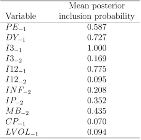
Table 1 provides the posterior mean for the probability of inclusion parameter

λj. We observe that the first lag of the 3-month T-Bill rate I3−1 is included with

probability 1. This perhaps is not surprising given that the dependent variable is the stock return in excess of the 3-month rate. The only other variables for which the posterior probability of inclusion is higher than the prior probability are the

first lag of 12-month T-bond rate I12−1 (0.775), the dividend yield DY−1 (0.727)

and the price-earnings ratioP E−1 (0.587). Obviously, bonds are alternative

invest-ments to stocks, in particular during bear markets, such that it is to be expected that they have some predictive power for stock returns. By contrast, the dividend yield is often referred to as an indicator of stock market performance. Note that the second lags of both interest rates have rather low posterior inclusion probabili-ties, indicating that movements in interest rates have substantially lower in-sample

predictive power than the interest rate levels. The credit spread CP−1 and stock

1_{We point out that the predictor variables are demeaned to exclude that possible breaks in the}

relation between the excess returns and some predictors imply also a breaks in the coefficient of the constant term.

return volatilityLV OL−1 have particular low posterior inclusion probabilities,

indi-cating that these variables have not been useful as predictors of stock returns over the sample period considered. Finally, all three macroeconomic variables have pos-terior inclusion probabilities slightly below the prior value of 0.5, suggesting lower predictive power than the financial variables.

Additional insight into the variable selection results can be obtained from the joint selection of different variables. For that purpose, Table 2 presents the poste-rior joint probabilities of inclusion for all possible pairs of variables. Note that the prior probability of joint inclusion for any two variables is equal to 0.25, given that all individual prior probabilities are equal to 0.5 and independent across variables. Table 3 shows the values of the measure of jointness results of Doppelhofer and Weeks (2005). Note that the jointness measure involving the 3-month T-Bill rate takes the value zero by construction. Obviously, the results in Table 2 partly follow directly from the variable-specific selection probabilities in Table 1. For example, given that the dividend yield and the two interest rate variables have such high indi-vidual probabilities of inclusion, their combinations have high posterior probability

to be selected together as well. The measure of jointness for (DY−1,I12−1) has a

correspondingly large value. The couple (P E−1,DY−1) has a posterior probability of

being selected together of 0.316, which is very close to the lower bound (0.314) that is possible given their individual inclusion probabilities. Although not borne out by their coefficient of jointness, this indicates that these variables are close substitutes. This is not surprising given that both the price-earnings ratio and the dividend yield are well-accepted valuation measures having similar predictive content for the

development of the stock market. For the monetary base growth variable MB−2

the posterior probability of joint inclusion with the dividend-yield, price-earnings ratio, and both short- and long-term interest rates is higher than its prior, while the corresponding jointness measures in Table 3 confirm that money growth is com-plementary to these financial variables. Almost all other combinations of variables have posterior probabilities lower than the prior value of 0.25. Nevertheless, the

jointness measures for industrial production growth IP−2 and volatility LV OL−1

indicate that these variables may include some useful information that complements the financial variables.

Finally, Table 4 provides the ten models which have the highest probabilities to be selected. The conclusions from this table agree with the findings from Tables 1-3

as discussed above. First, the variables I3−1 and I12−1 are always included in the

ratio P E−1 also enters the model, but these two variables are not often included

together because they are complements. Third, even though in several models one of the macro-economic variables is included, their importance does not seem very large. Finally, it is worth nothing that the sum of the posterior probabilities for these ten models is larger than 0.5, suggesting that financial variables are the most important predictor variables for stock returns.

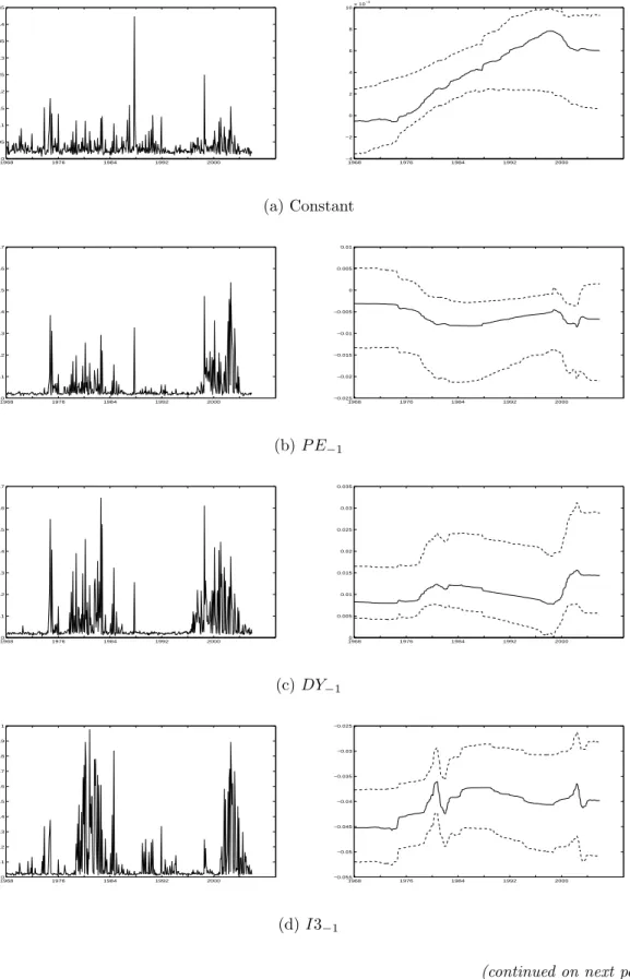
We now turn to the analysis of the regression parameters and possible structural breaks therein. Figure 1 shows the posterior mean for the latent binary variable

κjt governing the occurrence of changes in the regression parameters, together with

the associated posterior mean for βjt. For the latter, 25th and 75th percentiles of

the posterior distributions are also shown. One of the things that stands out most clearly from the graphs in Figure 1 is the spiky nature of the posterior mean of

κjt, suggesting that the probabilities of structural breaks in the parameters vary

considerably from one period to the next.2 _{This occurs for two reasons. First,}

κj,t can be different across different values of S, such that breaks can occur at

different times across models. Second, in case a break is estimated to have occurred in a certain month, the probability of a break in the next month will be much lower. Despite the volatile behavior of the break probabilities, three periods with considerable probability mass can be identified: during the years 1974-1975, around 1982 and around 2001. Political reasons and the oil price shocks provide possible explanations for the first break period. The change of the Federal Reserve’s operating procedures at the beginning of the 1980’s explain the second break, and the crash of the internet bubble the third one. Also note that the stock market crash in October 1987 gives rise to an isolated jump in the break probability for some variables

(notably the constantC, the price-earnings ratio P E−1, industrial productionIP−2,

the credit spread CP−1 and volatility LV OL−1). This seems to suggest that this

event did not give rise to a permanent change in the relationship between stock returns and the predictor variables, but rather is identified as an outlier.

The 25th-75th percentile bands for the regression parameters βjt in Figure 1 are

quite wide and furthermore, the magnitudes of the changes in the posterior mean when a break occurs do not seem very large. This is due to the fact that variables are not always selected in the model, and when they are not, values for their regression parameters are drawn from their prior distributions. This explains, for example, why the variables with a low probability to be selected have rather flat posterior means

2_{Recall that the posterior mean ofκ}

jtis identical to the posterior probability of a break occurring

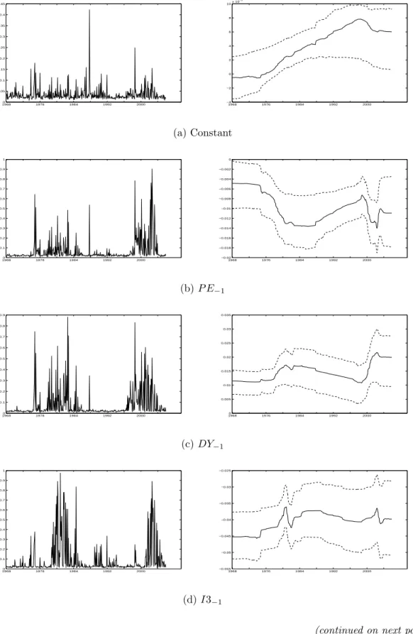
for βj,t, around the prior value. In Figure 2 we therefore consider the posterior

densities for κjt and βj,t conditional on inclusion of the variable j, that is sj = 1.

Obviously, the posterior probabilities of structural breaks are much higher in this case, while the magnitudes of the breaks become larger and vary considerably over the set of variables. Several interesting findings emerge. First, the pattern of the

interceptβ0t reveals a gradual increase in the unconditional equity premium during

the 1980s and 1990s, followed by a decline just before the turn of the millennium.

Second, for the price-earnings ratio P E−1 and the dividend yield DY−1 the most

substantial changes in parameters occur during the period 1999-2002 (in addition to

the drop in theP E−1 coefficient during the second half of the 1970s). These changes

reflect the large decline in the dividend yield and corresponding large increase in the price-earnings ratio due to the dramatic boom of stock prices during that period. Third, the largest breaks in the coefficients related to interest rates appear to have occurred around 1982, around the time the Federal Reserve changed its monetary policy. Fourth, the coefficients related to inflation and industrial production growth display the largest change around 1974, due to the oil price shocks and the higher level of inflation and slowdown in economic growth that followed. Fifth and finally, the coefficients of the monetary base and the credit spread display very large breaks at October 1987. Hence, contrary to our prior observation that the stock market crash probably is considered to be an outlier, it does seem to have led to structural breaks in at least some relationships between stock returns and predictor variables. In that respect, the pattern in the coefficient of volatility also is interesting, showing a gradual decline up to the moment of the crash, and a gradual increase thereafter.

4

Active investment strategies allowing for model

uncertainty and structural breaks

The full-sample results presented in the previous section provides a useful ex post

characterization of the (relative) importance of financial and macroeconomic vari-ables as predictors in return forecasting models and of possible breaks in the re-gression parameters. For an investor, both issues of variable selection and model

instability are most interesting from an ex ante perspective. That is, the relevant

questions are whether we can identify the appropriate predictor variables and detect structural breaks in regression parameters in real time, and how these may affect investment decisions. Answering these questions is the purpose of this section.

4.1

A utility-based performance measure

Several papers consider the effects of either model uncertainty or model instability on optimal asset allocation decisions, see Kandel and Stambaugh (1996), Barberis (2000), Avramov (2002) and Pettenuzzo and Timmermann (2005). Most of these analyses focus on horizon effects, that is the issue how uncertainty about the relevant predictor variables or the possibility of structural breaks changes the decisions of investors with different horizons, typically ranging from a single month up to ten years. Here we only consider an active short-term investor, with an investment horizon of one month. The investor’s portfolio consists of stocks and riskfree bonds

only. At the start of each monthT+ 1, the investor decides upon the fraction of her

portfolio to be invested in stocks wT+1, based upon a forecast of the excess stock

return rT+1. The investor is assumed to maximize a power utility function with

coefficient of relative risk aversion γ:

u(WT+1) =

W_T1−₊₁γ

1−γ, γ >0, (16)

whereWT+1 is the wealth at the end of period T + 1, which is equal to

WT+1 =WT((1−wT+1) exp(rf,T+1) +wT+1exp(rf,T+1+rT+1)), (17)

whereWT denotes initial wealth, and where rf,T+1 is the riskfree rate.

Without loss of generality we set initial wealth at one, WT = 1, such that the

investor’s optimization problem is given by max wT+1 ET(u(WT+1)) = max wT+1 ET µ ((1−wT+1) exp(rf,T+1) +wT+1exp(rf,T+1+rT+1))1−γ 1−γ ¶ , (18)

where ET is the conditional expectation given information at time T. How this

expectation is computed depends on the treatment of model uncertainty and model instability by the investor. Consider the most general case, both allowing for uncer-tainty concerning which predictor variables to include and allowing for the possibility of structural breaks in the regressions parameters, as given by model (5) with (4).

The marginal predictive density for future excess stock returns p(rT+1|r, x, xT+1) in

(15) should then be used to derive the proportion of the portfolio allocated to stocks according to (18). That is, the investor solves the following problem:

max

wT+1

Z

u(WT+1)p(rT+1|r, x, xT+1)drT+1. (19)

The integral in (19) is approximated by generating Gindependent draws {rg_T+1}G

g=1

optimization method to maximize the quantity: 1 G G X g=1 µ ((1−wT+1) exp(rf,T+1) +wT+1exp(rf,T+1+rTg+1))1−γ 1−γ ¶ (20) Two further cases are included in the empirical analysis below. First, we con-sider an investor who incorporates model uncertainty but ignores the possibility of structural breaks in the regression parameters. This investor obtains a forecast of

the excess stock return rT+1 from model (5) but with βjt = βj for j = 0,1, . . . , k

and t = 1, . . . , T + 1. Second, we consider an investor who also is ignorant about model uncertainty and simply includes all available predictor variables in the model, effectively using the benchmark model (1) for return forecasting.

As explained by Barberis (2000), the weight wT+1 in (17) cannot be left

uncon-strained in the optimization problem (18) as expected utility would be equal to−∞

in that case. We consider the following two restrictions on wT+1. First, we restrict

wT+1 ∈ [−1,2], allowing some extent of short-sales and leveraging of the

portfo-lio. Second, we do not allow for short-sales or leveraging at all, by constraining

wT+1 to be in the [0,1] interval. Hence, in total we consider six active investment

strategies. For comparison, we include three static benchmark strategies: I) holding stocks only, II) holding a portfolio consisting of 50% stocks and 50% bonds, and III) holding bonds only.

We evaluate the different investment strategies by computing the ex post utility

levels substituting the realized return of the portfolios at time T + 1 in (18). Total

utility is then obtained as the sum of u(WT+1) across all investment periods T =

T0, . . . , T0+T∗. In order to compare two alternative strategies we compute the return

that equates their average utilities. For example, suppose we compare the strategy based on excess return forecasts from the benchmark model (1) with a fixed set of predictor variables and constant regression parameters to the strategy based on the general model (5) with (4) that incorporates model uncertainty and structural

breaks. The wealth provided at timeT+ 1 by the two resulting portfolios is denoted

asW1,T+1 and W2,T+1, respectively. We then determine the value of ∆ such that

TX0+T∗ T=T0 u(W1,T+1) = TX0+T∗ T=T0 u(W2,T+1/exp(∆)). (21)

Following Fleming et al. (2001), we interpret ∆ as the maximum performance fee

the investor would be willing to pay to switch from the first strategy to the second. In that sense, ∆ represents the economic value of model uncertainty and model instability, in the example above.

Finally, the portfolio weights in the active investment strategies change every month, and the portfolio must be rebalanced accordingly. Hence, transaction costs play a non-trivial role and should be taken into account in evaluating the relative performance of different strategies. Rebalancing the portfolio at the start of month

T + 1 means that the weight invested in stocks is changed from wT to wT+1. We

assume that transaction costs amount to a fixed percentagecon each traded dollar.

Setting the initial wealthWT equal to 1 for simplicity, transaction costs at timeT+1

are equal to

cT+1 = 2c|wT+1−wT| (22)

where the multiplication by 2 follows from the fact that the investor rebalances her investments in both stocks and bonds. The net portfolio return is then given by

rT+1−cT+1. We apply two scenarios with transaction costs of 0.1% and 0.5%. Note

that for a passive strategy the inclusion of transaction costs matters only in buying the portfolio at the beginning.

4.2

Empirical Results

The analysis for the active investment strategies is implemented for the period from

January 1976 until December 2005, involving T∗ _{= 360 one month ahead return}

forecasts. The models are estimated recursively using an expanding window of

ob-servations, with the firstT = 120 months being used to estimate the initial models

that are used to obtain the first return prediction. The investment strategies are

implemented for two levels of relative risk aversion,γ = 5 and 10. Before we analyze

the performance of the different portfolios, we summarize the statistical accuracy of the forecasts of the excess stock returns.

The forecasts obtained from the model allowing for uncertainty concerning which predictor variables to include and allowing for the possibility of structural breaks in the regressions parameters (5) with (4) have mean error (ME) of 0.33% and a root mean square prediction error (RMSPE) of 4.58%. This is slightly more accurate than the linear and BMA forecasting models, both of which have RMSPEs equal to 4.64%. The ME of these models are 0.45% and 0.41%, respectively. Figure 3 shows five-year moving averages of the excess returns’ RMSPE and the hit ratio, defined as the proportion of correctly predicted signs. Both graphs show that the model performs quite well until October 1987. The stock market crash causes a large upward jump in the RMSPE, and marks the beginning of a period with less accurate forecasts and a steady decline in the hit ratio. Forecast accuracy improves again considerably during the period 1991-1997 with the RMSPE reaching a low of

just under 3% and the hit ratio peaking at 0.67. Predictability of the stock returns then deteriorates dramatically due to the internet bubble and its burst, and the hit ratio sharply drops to less than 0.4 in 2004. In sum, predictive accuracy varies considerably over time, even if a flexible forecast approach allowing for structural breaks and model uncertainty is employed.

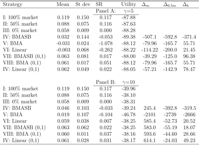
Table 5 provides summary statistics for the performance of the nine different investment strategies considered, ignoring transaction costs for the moment. In addition to the total utility levels and the performance fee ∆ relative to the buy-and-hold stock portfolio, we report traditional performance measures including the annualized mean and standard deviation of portfolio returns, and the Sharpe ratio (computed as the ratio of the mean monthly excess return on the portfolio and the monthly standard deviation of the portfolio return).

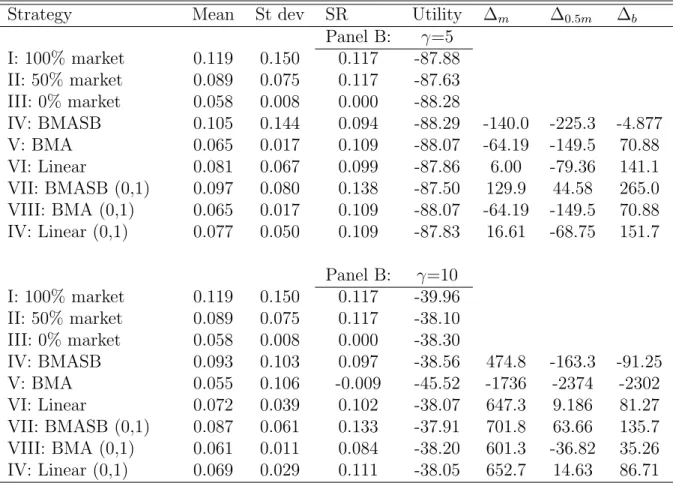
Over the complete investment period from January 1976 until December 2005, the average annualized return on the buy-and-hold stock portfolio is 11.91% with an estimated unconditional standard deviation of 15%, while the bonds portfolio pro-vides a mean return of 5.82% with a standard deviation of 0.85%. The Sharpe ratio of the stock portfolio is 0.117, while for the bond portfolio it is zero by construction. In terms of utility levels, the buy-and-hold mixed portfolio consisting of 50% stocks and 50% bonds renders the best results.

Next consider the active investment strategies based on excess return forecasts that account for model uncertainty and breaks (Strategies IV and VII). We observe that these all render lower average returns than the buy-and-hold stock portfolio. At the same time, portfolio risk is reduced considerably as well. For example, the restricted portfolios render return standard deviations that are 8.0% and 6.1% for

γ = 5 and 10, respectively, compared to 15% for the passive stock portfolio. This

reduction in volatility comes at the cost of lower mean returns by 2.2% and 3.2% for low and high risk averse investors, respectively. Despite this substantial return sacrifice, the Sharpe ratios of the active portfolios are higher at 0.138 and 0.133. The benefits of the active investment strategy also are revealed clearly by the performance fee ∆. We find that the investor would be willing to pay 130 and 700 basis points to switch from the passive to the active strategy. The passive mixed portfolio is outperformed as well, although the estimates of ∆ are considerably lower at 45 and 64 basis points. The reduction in average returns is less for the unrestricted portfolios, but the corresponding reduction of return volatility also is much smaller such that the resulting Sharpe ratios are below that of the passive stock portfolio.

higher utility, resulting in a negative performance fee of −140 basispoints for the active strategy. The high risk averse still prefers the active strategy though, and would be willing to pay 475 basis points annually to trade it against the buy-and-hold stock portfolio.

The performance of the other active investment strategies based on excess return forecasts from more restricted models is less convincing. Although these strategies lower the volatility of portfolio returns even more than the strategy based on forecasts from the general model, the reduction in average returns is considerably larger as well. For example, the restricted portfolio based on excess return forecasts from the model that only accounts for model uncertainty but ignores structural breaks (Strategy VIII) renders volatility of 1.1% but at a mean return of only 6.1% for

γ = 10. In all cases the resulting Sharpe ratios is lower compared to the portfolios

based on the general model. Also in terms of the utility levels and performance fee, Strategy VII achieves the best performance.

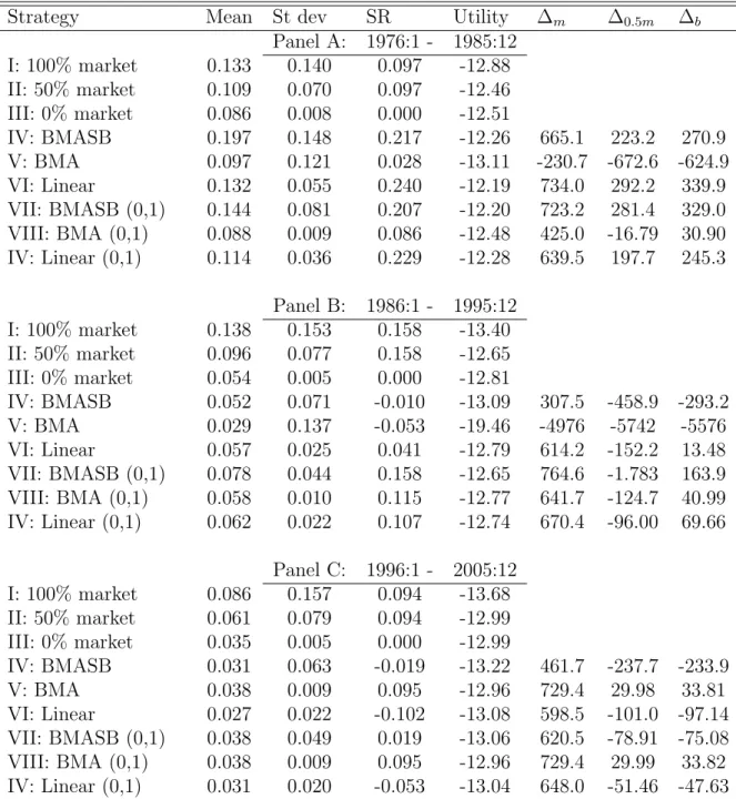
Figure 3 suggests that the accuracy of the excess return forecasts varies consider-ably over time. How this affects the performance of the active strategies can be seen from Table 6, which shows performance statistics for three sub-periods each covering

a decade for the investor with high relative risk aversion (γ = 10).3 _{We focus on the}

restricted active portfolios that results from forecasts of the general model allowing for model uncertainty and structural breaks (Strategy VII). Its performance is quite impressive during the first decade of the investment period, from January 1976 until December 1985, with a Sharpe ratio of 0.207, more than double the Sharpe ratios of the passive portfolios held in Strategies I and II. This is due to the fact that the mean return of the active strategy during this period is actually higher than the mean return of the buy-and-hold portfolio (14.4% compared to 13.2%), while volatility is reduced by about 40%. The corresponding performance fees are positive and large. The Sharpe ratios of the active and passive strategies are exactly equal during the second decade from January 1986 until December 1995, although in terms of utility level the buy-and-hold stock portfolio is still outperformed by the active strategy. The mixed portfolio achieves exactly the same level of utility however, resulting in a performance fee close to zero. The active strategy’s performance dete-riorates during the third and final decade, from January 1996 until December 2005. Although the reduction in portfolio returns’ volatility is of the same magnitude as before, the loss in average return is much larger. This results in a Sharpe ratio of

3_{Sub-sample results for the investor with low relative risk aversion (γ = 5) are qualitatively}

0.019, compared to 0.094 for the passive portfolios. It is quite remarkable then that the active strategy still achieved higher utility than the buy-and-hold stock portfolio

(−13.06 compared to −13.68). The mixed passive portfolio in turn renders higher

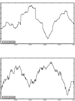
utility than the active strategy, resulting in a negative performance fee. In sum, it seems that the performance of the active strategies has gradually declined over time. Our analysis of the active investment strategies so far has ignored transaction costs. Obviously, their effects on the strategies; performance crucially depends on the average absolute change in portfolio weights, see (22). Figure 4 shows the portfolio weight for stocks in the restricted portfolios based on excess stock return forecasts from the general model, allowing for model uncertainty and structural breaks in the regression parameters (Strategy VII). Although there are extended periods of time when the investment in stocks is at high or low levels, month-to-month variation in the portfolio weight seems quite substantial. Hence, a proper analysis of the effects of transaction costs is warranted.

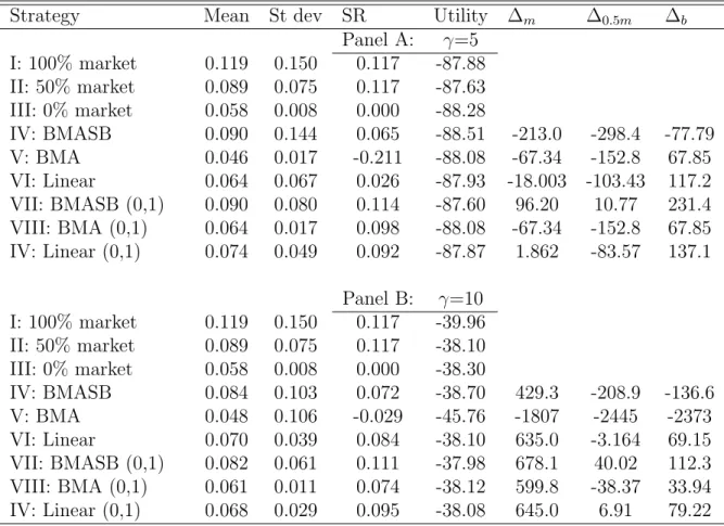
Tables 8 and 8 present results for the complete 30-year investment period for low (0.1%) and moderate (0.5%) levels of transaction costs, respectively. The pres-ence of transaction costs obviously hurts the active strategies’ performance. For low transaction cost levels, the restricted portfolio based on return forecasts from the general model continues to outperform the buy-and-hold stock and mixed portfolios, although the performance fees ∆ become somewhat lower. For moderate transaction cost levels, only the high risk averse investor prefers the active strategy over the pas-sive stock portfolio. For both levels of risk aversion considered, the mixed portfolio renders superior results on all measures considered: it has higher mean return, lower volatility (and thus a higher Sharpe ratio) and higher utility.

5

Conclusion

Optimal portfolio decisions force investors to make a number of important decisions concerning the return forecasting model used. These decisions involve in particu-lar the treatment of different sources of uncertainty, about the relevant predictor variables (model uncertainty), the values of the regression parameters (parameter uncertainty), and their stability (structural breaks). In this paper we have devel-oped a framework to incorporate all three sources of uncertainty simultaneously. This extends previous research allowing for either parameter uncertainty and model uncertainty (Avramov (2002), Cremers (2002)), or parameter uncertainty and

Our empirical results suggest, first, that over the period 1966-2005, several struc-tural breaks occurred in the relationship between US stock returns and predictor variables such as the dividend yield and interest rates. These changes appear to be caused by important events such as the oil crisis, changes in monetary policy, and the October 1987 stock market crash. Second, we find that allowing for model un-certainty, and structural breaks has considerable economic value. A typical investor would be willing to pay up to several hundreds of basis points annually to switch from a passive buy-and-hold strategy to an active strategy based on a return fore-casting model that allows for model and parameter uncertainty as well as structural breaks in the regression parameters. The active strategy that incorporates all three sources of uncertainty performs considerably better than strategies based on more restricted return forecasting models.

References

Akgiray, V. (1989), Conditional Heteroskedasticity in Time Series of Stock Returns: Evi-dences and Forecasts, Journal of Business,62, 55–80.

Avramov, D. (2002), Stock Return Predictability and Model Uncertainty,Journal of Fi-nancial Economics,64, 423–458.

Barberis, N. (2000), Investing for the Long Run When Returns Are Predictable, Journal of Finance,55, 225–264.

Carter, C. and R. Kohn (1994), On Gibbs Sampling for State-Space Models,Biometrika, 81, 541–553.

Cremers, K. (2002), Stock Return Predictability: A Bayesian Model Selection Perspective,

Review of Financial Studies,15, 1223–1249.

Doppelhofer, G. and M. Weeks (2005), Jointness of Growth Determinants,Working paper. Fern´andez, C., E. Ley, and M. Steel (2001), Benchmark priors for Bayesian model

averag-ing, Journal of Econometrics, 381–427.

Fleming, J., C. Kirby, and B. Ostdiek (2001), The Economic Value of Volatility Timing,

Journal of Finance,56, 329–352.

French, K., G. Schwert, and R. Stambaugh (1987), Expcted Stock Returns and Volatility,

Journal of Financial Economics,19, 3–29.

Geman, S. and D. Geman (1984), Stochastic Relaxation, Gibbs Distributions and the Bayesian Restoration of Images, IEEE Transaction on Pattern Analysis and Machine Intelligence,6, 721–741.

George, E. I. and R. E. McCulloch (1993), Variable Selection Via Gibbs Sampling,Journal of the American Statistical Association,88, 881–889.

Gerlach, R., C. Carter, and R. Kohn (2000), Efficient Bayesian Inference for Dynamic Mixture Models, Journal of the American Statistical Association,95, 819–828.

Giordani, P., R. Kohn, and D. van Dijk (2006), A Unified Approach to Nonlinearity, Outliers and Structural Breaks, Journal of Econometrics, to appear.

Kandel, S. and R. Stambaugh (1996), On the Predictability of Stock Returns: An Asset Allocation Perspective, Journal of Finance,51, 385–424.

Koop, G. and S. Potter (2004), Forecasting and Estimating Multiple Change-point Models with an Unknown Number of Change-points,Working paper.

Kuo, L. and B. Mallick (1998), Variable Selection for Regression Models, The Indian Journal of Statistics,60, 65–81.

Marquering, W. and M. Verbeek (2004), The Economic Value of Predicting Stock Index Returns and Volatility, Journal of Financial and Quantitative Analysis, 39 (2), 407– 429.

Pesaran, M., D. Pettenuzzo, and A. Timmermann (2004), Forecasting Time Series Subject to Multiple Structural Breaks, Working paper.

Pesaran, M. and A. Timmermann (2002), Market Timing and Return Predictability Under Model Instability,Journal of Empirical Finance,9, 495–510.

Pettenuzzo, D. and A. Timmermann (2005), Predictability of Stock Returns and Asset Allocation under Structural Breaks, Working paper.

Tanner, M. and W. Wong (1987), The Calculation of Posterior Distributions by Data Augmentation, Journal of the American Statistical Association,82, 528–550.

Table 1: Probability of variable selec-tion

Mean posterior

Variable inclusion probability

P E−1 0.587 DY−1 0.727 I3−1 1.000 I3−2 0.169 I12−1 0.775 I12−2 0.095 INF−2 0.208 IP−2 0.352 MB−2 0.435 CP−1 0.070 LV OL−1 0.094

The table presents the marginal poste-rior probability of any single explanatory variable to be selected.

T able 2: P osterior probabilit y of join t selection P E− 1 D Y− 1 I 3− 1 I 3− 2 I 12− 1 I 12− 2 IN F− 2 IP − 2 M B− 2 C P− 1 LV O L− 1 C 0.587 0.727 1.000 0.169 0.775 0.095 0.208 0.352 0.435 0.070 0.094 P E− 1 0.319 0.587 0.017 0.522 0.095 0.124 0.285 0.278 0.034 0.044 D Y− 1 0.727 0.169 0.541 0.035 0.126 0.185 0.321 0.069 0.076 I 3−1 0.169 0.775 0.095 0.208 0.352 0.435 0.070 0.094 I 3−2 0.050 0.000 0.021 0.013 0.000 0.050 0.003 I 12− 1 0.030 0.134 0.300 0.341 0.070 0.090 I 12− 2 0.021 0.035 0.093 0.000 0.000 IN F− 2 0.117 0.110 0.004 0.004 IP − 2 0.155 0.014 0.009 M B− 2 0.003 0.073 C P− 1 0.003 The table presen ts p osterior probabilit y of couples of explanatory variables to b e selected.

T able 3: Biv ariate join tness among tw o regressors D Y− 1 I 3− 1 I 3−2 I 12− 1 I 12− 2 IN F− 2 IP − 2 M B− 2 C P− 1 LV O L− 1 P E− 1 -0.291 -0.214 -2.297 1.383 0.255 1.837 1.359 0.596 0.110 1.900 D Y− 1 0.000 0.000 1.418 -0.744 1.853 0.927 0.740 0.818 2.447 I 3−1 0.000 0.000 0.000 0.000 0.000 0.000 0.000 0.000 I 3−2 -0.963 0.000 0.061 -1.728 0.000 0.496 -0.785 I 12− 1 -0.898 1.914 1.410 0.801 0.832 2.616 I 12− 2 0.061 -0.738 -0.499 0.000 0.000 IN F− 2 0.469 -0.331 -2.030 -0.498 IP − 2 0.012 -0.777 0.313 M B− 2 -2.317 2.406 C P− 1 -0.785 The table presen ts the degree of dep endence or join tness among couples of explanatory variables.

T able 4: P osterior mo del probabilities Mo del P osterior probabilit y C , D Y− 1 , I 3− 1 , I 3− 2 0.0950 C , D Y− 1 , I 3− 1 , I 12− 1 , M B− 2 0.0810 C , P E− 1 , D Y− 1 , I 3− 1 , I 12− 1 0.0670 C , P E− 1 , I 3−1 , I 12− 2 , IP − 2 0.0560 C , P E− 1 , I 3−1 , I 12− 1 0.0480 C , P E− 1 , D Y− 1 , I 3− 1 , I 12− 1 , IP − 2 0.0430 C , D Y− 1 , I 3− 1 , I 12− 1 0.0380 C , P E− 1 , D Y− 1 , I 3− 1 , I 12− 1 , M B− 2 0.0370 C , D Y− 1 , I 3− 1 , I 12− 1 , M B− 2 , LV O L− 1 0.0370 C , P E− 1 , D Y− 1 , I 3− 1 , I 12− 1 , IP − 2 , M B− 2 0.0340 The table lists the ten mo dels with highest p osterior probabilities and the resp ec-tiv e probabilities.

Table 5: No transaction costs

Strategy Mean St dev SR Utility ∆m ∆0.5m ∆b

Panel B: γ=5 I: 100% market 0.119 0.150 0.117 -87.88 II: 50% market 0.089 0.075 0.117 -87.63 III: 0% market 0.058 0.008 0.000 -88.28 IV: BMASB 0.105 0.144 0.094 -88.29 -140.0 -225.3 -4.877 V: BMA 0.065 0.017 0.109 -88.07 -64.19 -149.5 70.88 VI: Linear 0.081 0.067 0.099 -87.86 6.00 -79.36 141.1 VII: BMASB (0,1) 0.097 0.080 0.138 -87.50 129.9 44.58 265.0 VIII: BMA (0,1) 0.065 0.017 0.109 -88.07 -64.19 -149.5 70.88 IV: Linear (0,1) 0.077 0.050 0.109 -87.83 16.61 -68.75 151.7 Panel B: γ=10 I: 100% market 0.119 0.150 0.117 -39.96 II: 50% market 0.089 0.075 0.117 -38.10 III: 0% market 0.058 0.008 0.000 -38.30 IV: BMASB 0.093 0.103 0.097 -38.56 474.8 -163.3 -91.25 V: BMA 0.055 0.106 -0.009 -45.52 -1736 -2374 -2302 VI: Linear 0.072 0.039 0.102 -38.07 647.3 9.186 81.27 VII: BMASB (0,1) 0.087 0.061 0.133 -37.91 701.8 63.66 135.7 VIII: BMA (0,1) 0.061 0.011 0.084 -38.20 601.3 -36.82 35.26 IV: Linear (0,1) 0.069 0.029 0.111 -38.05 652.7 14.63 86.71

The table presents the annualized average % return, the annualized standard deviation, the Sharpe ratio (SR), and the utility value of the 9 different strategies for the full forecasting sample period 1976:1-2005:12. The last 3 columns present the annualized return in basis points that an active strategy gives in surplus of the return of a passive strategy.

Table 6: Subperiods,γ = 10

Strategy Mean St dev SR Utility ∆m ∆0.5m ∆b

Panel A: 1976:1 - 1985:12 I: 100% market 0.133 0.140 0.097 -12.88 II: 50% market 0.109 0.070 0.097 -12.46 III: 0% market 0.086 0.008 0.000 -12.51 IV: BMASB 0.197 0.148 0.217 -12.26 665.1 223.2 270.9 V: BMA 0.097 0.121 0.028 -13.11 -230.7 -672.6 -624.9 VI: Linear 0.132 0.055 0.240 -12.19 734.0 292.2 339.9 VII: BMASB (0,1) 0.144 0.081 0.207 -12.20 723.2 281.4 329.0 VIII: BMA (0,1) 0.088 0.009 0.086 -12.48 425.0 -16.79 30.90 IV: Linear (0,1) 0.114 0.036 0.229 -12.28 639.5 197.7 245.3 Panel B: 1986:1 - 1995:12 I: 100% market 0.138 0.153 0.158 -13.40 II: 50% market 0.096 0.077 0.158 -12.65 III: 0% market 0.054 0.005 0.000 -12.81 IV: BMASB 0.052 0.071 -0.010 -13.09 307.5 -458.9 -293.2 V: BMA 0.029 0.137 -0.053 -19.46 -4976 -5742 -5576 VI: Linear 0.057 0.025 0.041 -12.79 614.2 -152.2 13.48 VII: BMASB (0,1) 0.078 0.044 0.158 -12.65 764.6 -1.783 163.9 VIII: BMA (0,1) 0.058 0.010 0.115 -12.77 641.7 -124.7 40.99 IV: Linear (0,1) 0.062 0.022 0.107 -12.74 670.4 -96.00 69.66 Panel C: 1996:1 - 2005:12 I: 100% market 0.086 0.157 0.094 -13.68 II: 50% market 0.061 0.079 0.094 -12.99 III: 0% market 0.035 0.005 0.000 -12.99 IV: BMASB 0.031 0.063 -0.019 -13.22 461.7 -237.7 -233.9 V: BMA 0.038 0.009 0.095 -12.96 729.4 29.98 33.81 VI: Linear 0.027 0.022 -0.102 -13.08 598.5 -101.0 -97.14 VII: BMASB (0,1) 0.038 0.049 0.019 -13.06 620.5 -78.91 -75.08 VIII: BMA (0,1) 0.038 0.009 0.095 -12.96 729.4 29.99 33.82 IV: Linear (0,1) 0.031 0.020 -0.053 -13.04 648.0 -51.46 -47.63

The table presents the annualized average % return, the annualized standard deviation, the Sharpe ratio (SR), and the utility value of the 9 strategies for the full forecasting sample period 1986:1-1995:12. The last 3 columns present the annualized return in basis points that an active strategy gives in surplus of the return of a passive strategy.

Table 7: 0.1% transaction costs

Strategy Mean St dev SR Utility ∆m ∆0.5m ∆b

Panel A: γ=5 I: 100% market 0.119 0.150 0.117 -87.88 II: 50% market 0.089 0.075 0.117 -87.63 III: 0% market 0.058 0.008 0.000 -88.28 IV: BMASB 0.090 0.144 0.065 -88.51 -213.0 -298.4 -77.79 V: BMA 0.046 0.017 -0.211 -88.08 -67.34 -152.8 67.85 VI: Linear 0.064 0.067 0.026 -87.93 -18.003 -103.43 117.2 VII: BMASB (0,1) 0.090 0.080 0.114 -87.60 96.20 10.77 231.4 VIII: BMA (0,1) 0.064 0.017 0.098 -88.08 -67.34 -152.8 67.85 IV: Linear (0,1) 0.074 0.049 0.092 -87.87 1.862 -83.57 137.1 Panel B: γ=10 I: 100% market 0.119 0.150 0.117 -39.96 II: 50% market 0.089 0.075 0.117 -38.10 III: 0% market 0.058 0.008 0.000 -38.30 IV: BMASB 0.084 0.103 0.072 -38.70 429.3 -208.9 -136.6 V: BMA 0.048 0.106 -0.029 -45.76 -1807 -2445 -2373 VI: Linear 0.070 0.039 0.084 -38.10 635.0 -3.164 69.15 VII: BMASB (0,1) 0.082 0.061 0.111 -37.98 678.1 40.02 112.3 VIII: BMA (0,1) 0.061 0.011 0.074 -38.12 599.8 -38.37 33.94 IV: Linear (0,1) 0.068 0.029 0.095 -38.08 645.0 6.91 79.22

The table presents the annualized average % return, the annualized standard deviation, the Sharpe ratio (SR), and the utility value of the 9 different strategies for the full forecasting sample period 1976:1-2005:12 with transaction cost of 0.1%. The last 3 columns present the annualized return in basis points that an active strategy gives in surplus of the return of a passive strategy.

Table 8: 0.5% transaction costs

Strategy Mean St dev SR Utility ∆m ∆0.5m ∆b

Panel A: γ=5 I: 100% market 0.119 0.150 0.117 -87.88 II: 50% market 0.088 0.075 0.116 -87.63 III: 0% market 0.058 0.009 0.000 -88.28 IV: BMASB 0.032 0.144 -0.053 -89.38 -507.1 -592.8 -371.4 V: BMA -0.031 0.024 -1.078 -88.12 -79.96 -165.7 55.71 VI: Linear -0.003 0.068 -0.262 -88.22 -114.22 -200.0 21.45 VII: BMASB (0,1) 0.063 0.081 0.017 -88.00 -39.29 -125.0 96.38 VIII: BMA (0,1) 0.061 0.017 0.051 -88.12 -79.96 -165.7 55.71 IV: Linear (0,1) 0.062 0.049 0.022 -88.05 -57.21 -142.9 78.47 Panel B: γ=10 I: 100% market 0.119 0.150 0.117 -39.96 II: 50% market 0.088 0.075 0.116 -38.10 III: 0% market 0.058 0.009 0.000 -38.31 IV: BMASB 0.046 0.103 -0.033 -39.24 245.4 -392.8 -319.5 V: BMA 0.019 0.107 -0.104 -46.78 -2101 -2739 -2666 VI: Linear 0.059 0.038 0.007 -38.25 585.4 -52.73 20.52 VII: BMASB (0,1) 0.063 0.062 0.022 -38.25 583.0 -55.19 18.07 VIII: BMA (0,1) 0.060 0.011 0.037 -38.16 593.6 -44.60 28.66 IV: Linear (0,1) 0.061 0.028 0.031 -38.17 614.1 -24.03 49.23

The table presents the annualized average % return, the annualized standard deviation, the Sharpe ratio (SR), and the utility value of the 9 different strategies for the full forecasting sample period 1976:1-2005:12 with transaction cost of 0.5%. The last 3 columns present the annualized return in basis points that an active strategy gives in surplus of the return of a passive strategy.

Figure 1: Marginal posterior densities of the breaks and β parameters 19680 1976 1984 1992 2000 0.05 0.1 0.15 0.2 0.25 0.3 0.35 0.4 0.45 1968 1976 1984 1992 2000 −4 −2 0 2 4 6 8 10x 10 −3 (a) Constant 19680 1976 1984 1992 2000 0.1 0.2 0.3 0.4 0.5 0.6 0.7 1968 1976 1984 1992 2000 −0.025 −0.02 −0.015 −0.01 −0.005 0 0.005 0.01 (b)P E−1 19680 1976 1984 1992 2000 0.1 0.2 0.3 0.4 0.5 0.6 0.7 19680 1976 1984 1992 2000 0.005 0.01 0.015 0.02 0.025 0.03 0.035 (c)DY−1 19680 1976 1984 1992 2000 0.1 0.2 0.3 0.4 0.5 0.6 0.7 0.8 0.9 1 1968 1976 1984 1992 2000 −0.055 −0.05 −0.045 −0.04 −0.035 −0.03 −0.025 (d)I3−1

19680 1976 1984 1992 2000 0.02 0.04 0.06 0.08 0.1 0.12 0.14 0.16 1968 1976 1984 1992 2000 −0.03 −0.02 −0.01 0 0.01 0.02 0.03 0.04 (e) I3−2 19680 1976 1984 1992 2000 0.1 0.2 0.3 0.4 0.5 0.6 0.7 19680 1976 1984 1992 2000 0.005 0.01 0.015 0.02 0.025 0.03 0.035 (f)I12−1 19680 1976 1984 1992 2000 0.02 0.04 0.06 0.08 0.1 0.12 1968 1976 1984 1992 2000 −0.04 −0.03 −0.02 −0.01 0 0.01 0.02 0.03 0.04 (g)I12−2 19680 1976 1984 1992 2000 0.05 0.1 0.15 0.2 0.25 1968 1976 1984 1992 2000 −0.025 −0.02 −0.015 −0.01 −0.005 0 0.005 0.01 0.015 0.02 0.025 (h)IN F−2

19680 1976 1984 1992 2000 0.05 0.1 0.15 0.2 0.25 1968 1976 1984 1992 2000 −0.02 −0.015 −0.01 −0.005 0 0.005 0.01 0.015 0.02 (i)IP−2 19680 1976 1984 1992 2000 0.05 0.1 0.15 0.2 0.25 0.3 0.35 1968 1976 1984 1992 2000 −0.02 −0.015 −0.01 −0.005 0 0.005 0.01 (j)M B−2 19680 1976 1984 1992 2000 0.01 0.02 0.03 0.04 0.05 0.06 0.07 0.08 0.09 1968 1976 1984 1992 2000 −0.03 −0.02 −0.01 0 0.01 0.02 0.03 0.04 (k)CP−1 19680 1976 1984 1992 2000 0.01 0.02 0.03 0.04 0.05 0.06 0.07 0.08 1968 1976 1984 1992 2000 −0.04 −0.03 −0.02 −0.01 0 0.01 0.02 0.03 (l)LV OL−1

Note: The figure presents the posterior means (solid line) of κjt on the left side andβjt on the

Figure 2: Posterior densities of the breaks andβparameters conditional on inclusion 19680 1976 1984 1992 2000 0.05 0.1 0.15 0.2 0.25 0.3 0.35 0.4 0.45 1968 1976 1984 1992 2000 −4 −2 0 2 4 6 8 10x 10 −3 (a) Constant 19680 1976 1984 1992 2000 0.1 0.2 0.3 0.4 0.5 0.6 0.7 0.8 0.9 1 1968 1976 1984 1992 2000 −0.02 −0.018 −0.016 −0.014 −0.012 −0.01 −0.008 −0.006 −0.004 −0.002 0 (b)P E−1 19680 1976 1984 1992 2000 0.1 0.2 0.3 0.4 0.5 0.6 0.7 0.8 0.9 19680 1976 1984 1992 2000 0.005 0.01 0.015 0.02 0.025 0.03 0.035 (c)DY−1 19680 1976 1984 1992 2000 0.1 0.2 0.3 0.4 0.5 0.6 0.7 0.8 0.9 1 1968 1976 1984 1992 2000 −0.055 −0.05 −0.045 −0.04 −0.035 −0.03 −0.025 (d)I3−1

19680 1976 1984 1992 2000 0.1 0.2 0.3 0.4 0.5 0.6 0.7 0.8 0.9 1968 1976 1984 1992 2000 0.015 0.02 0.025 0.03 0.035 0.04 0.045 0.05 (e) I3−2 19680 1976 1984 1992 2000 0.1 0.2 0.3 0.4 0.5 0.6 0.7 0.8 0.9 1968 1976 1984 1992 2000 0.005 0.01 0.015 0.02 0.025 0.03 0.035 (f)I12−1 19680 1976 1984 1992 2000 0.1 0.2 0.3 0.4 0.5 0.6 0.7 0.8 0.9 1 1968 1976 1984 1992 2000 0.005 0.01 0.015 0.02 0.025 0.03 0.035 (g)I12−2 19680 1976 1984 1992 2000 0.1 0.2 0.3 0.4 0.5 0.6 0.7 0.8 0.9 1 1968 1976 1984 1992 2000 −8 −6 −4 −2 0 2 4x 10 −3 (h)IN F−2