Improving Automatic Speech Recognition on Endangered Languages

Rochester Institute of Technology Rochester Institute of Technology

RIT Scholar Works

RIT Scholar Works

Theses

11-2019

Improving Automatic Speech Recognition on Endangered

Improving Automatic Speech Recognition on Endangered

Languages

Languages

Kruthika Prasanna Simha [email protected]

Follow this and additional works at: https://scholarworks.rit.edu/theses

Recommended Citation Recommended Citation

Simha, Kruthika Prasanna, "Improving Automatic Speech Recognition on Endangered Languages" (2019). Thesis. Rochester Institute of Technology. Accessed from

This Thesis is brought to you for free and open access by RIT Scholar Works. It has been accepted for inclusion in Theses by an authorized administrator of RIT Scholar Works. For more information, please contact

Improving Automatic Speech

Recognition on Endangered

Languages

Improving Automatic Speech

Recognition on Endangered

Languages

Kruthika Prasanna Simha November

2019

KATE GLEASON COLLEGE OF ENGINEERING A Thesis Submitted in Partial

Fulfillment

of the Requirements for the Degree of Master of Science in

Computer Engineering

Improving Automatic Speech Recognition

on Endangered Languages

By

Kruthika Prasanna Simha

November 2019

A Thesis Submitted in Partial Fulfillment of the Requirements for the Degree of Master of Science

in Computer Engineering from Rochester Institute of Technology

Approved by:

Dr. Raymond Ptucha, Assistant Professor Date

Thesis Advisor, Department of Computer Engineering

Dr. Cecilia Ovesdotter Alm, Associate Professor Date Thesis Advisor, Department of English

Dr. Andres Kwasinski, Professor Date

Committee Member, Department of Computer Engineering

i

Acknowledgements

I am very grateful to Dr. Ptucha for his constant encouragement, support and guidance throughout my master’s education. I would like to extend my gratitude towards Robbie Jimerson for giving me the opportunity to be involved in research on endangered languages, and to have supported me through my thesis. I would also like to thank my fellow Machine Intelligence Laboratory members for their support. And lastly, I would like to thank my family for giving me the opportunity to travel far from home to pursue my master’s degree.

ii

Abstract

As the world moves towards a more globalized scenario, it has brought along with it the extinction of several languages. It has been estimated that over the next century, over half of the world’s languages will be extinct, and an alarming 43% of the world’s languages are at different levels of endangerment or extinction already. The survival of many of these languages depends on the pressure imposed on the dwindling speakers of these languages. Often there is a strong correlation between endangered languages and the number and quality of recordings and documentations of each. But why do we care about preserving these less prevalent languages? The behavior of cultures is often expressed in the form of speech via one’s native language. The memories, ideas, major events, practices, cultures and lessons learnt, both individual as well as the community’s, are all communicated to the outside world via language. So, language preservation is crucial to understanding the behavior of these communities.

Deep learning models have been shown to dramatically improve speech recognition accuracy but require large amounts of labelled data. Unfortunately, resource constrained languages typically fall short of the necessary data for successful training. To help alleviate the problem, data augmentation techniques fabricate many new samples from each sample. The aim of this master’s thesis is to examine the effect of different augmentation techniques on speech recognition of resource constrained languages. The augmentation methods being experimented with are noise augmentation, pitch augmentation, speed augmentation as well as voice transformation augmentation using Generative Adversarial Networks (GANs). This thesis also examines the effectiveness of GANs in voice transformation and its limitations. The information gained from this study will further augment the collection of data, specifically, in understanding the conditions required for the data to be collected in, so that GANs can effectively perform voice

iii

transformation. Training of the original data on the Deep Speech model resulted in 95.03% WER. Training the Seneca data on a Deep Speech model that was pretrained on an English dataset, reduced the WER to 70.43%. On adding 15 augmented samples per sample, the WER reduced to 68.33%. Finally, adding 25 augmented samples per sample, the WER reduced to 48.23%. Experiments to find the best augmentation method among noise addition, pitch variation, speed variation augmentation and GAN augmentation revealed that GAN augmentation performed the best, with a WER reduction to 60.03%.

iv

Table of Contents

Chapter

Number

Name of Chapter

Page

Number

1. Introduction 1

2. Related Work 4

3. Background 8

3.1. Under-Resourced Languages 8

3.2. Automatic Speech Recognition 9

3.2.1. Feature Extraction 9

3.2.2. Acoustic Modeling 10

3.2.3. Language Modeling 10

3.2.4. Lexical Modeling 11

3.3. Mel Frequency Cepstral Coefficients 11

3.3.1. Pre-emphasis 11

3.3.2. Windowing 12

3.3.3. Discrete Fourier Transform 12

3.3.4. Mel Filter Bank and Log 12

3.3.5. The Cepstrum 13

3.4. The Deep Speech Model 14

4. Generative Adversarial Networks 16

4.1. Generative Adversarial Networks Preliminaries 16

4.2. CycleGAN 17

4.3. DiscoGAN and CycleGAN vs DiscoGAN 19

4.4. VoiceGAN 20

4.4.1. Image vs Speech samples 20

4.4.2. VoiceGAN model changes 21

v

4.4.2.2. Variable-length input generator and discriminator 22

4.4.2.3. Style Embedding Model 22

4.5. StarGAN-VC 23

4.5.1. Objectives 23

4.5.1.1. Adversarial Loss 25

4.5.1.2. Domain Classification Loss 25

4.5.1.3. Cycle Consistency Loss 25

4.6. StarGAN-VC v/s VoiceGAN 26

5. Raw Audio, Spectrogram and MFCCs 27

5.1. What is raw audio format? 27

5.2. What are Spectrograms? 27

5.2.1. Wideband and Narrowband Spectrograms 28

5.3. Computing the Spectrogram 30

5.3.1. Input Values to Deep Speech 31

5.4. Converting Spectrogram to Raw Audio 31

5.5. Computing MFCCs from a Spectrogram 33

6. Thesis Proposal 34

6.1. Problem Statement 34

6.2. Dataset 34

6.2.1. Seneca Dataset 34

6.2.2. Free Spoken Digits Dataset 36

6.2.3. LibriSpeech 36

6.2.4. Tensorflow Speech Recognition Challenge Dataset 36 6.2.5. Voice Conversion Challenge 2018 Parallel Dataset 37

6.3. Language Model 37

6.4. Data Augmentation 37

6.4.1. Noise Addition 37

vi

6.4.3. Speed Augmentation 40

6.5. Research Questions 40

7. Design of Experiments 41

7.1. Problem Statement and Hypothesis 41

7.2. Design of Experiments 42

7.2.1. Deep Speech Experiments 42

7.2.2. Griffin-Lim Algorithm Experiments 45

7.2.3. VoiceGAN Experiments 45

7.2.4. StarGAN-VC Experiments 50

7.3. Morpheme error rate v/s Word error rate 51

7.4. Motivation behind chosen augmentation techniques 51

8. Results and Inferences 53

8.1. Deep Speech 53

8.1.1. Data Augmentation 53

8.1.1.1. Noise Addition 53

8.1.1.2. Pitch Augmentation 54

8.1.1.3. Speed Augmentation 56

8.1.2. Deep Speech Results and Inference 58

8.2. Griffin-Lim Algorithm experiments 60

8.3. VoiceGAN results 61

8.3.1. LibriSpeech results and observations 62

8.3.2. Free 0-9 dataset results and observations 63

8.3.3. TSRC results and observations 67

8.3.4. StarGAN-VC augmentation results with DeepSpeech 68

8.3.5. Inference 69

9. Conclusion and Future Work 70

9.1. Conclusion 70

vii

List of Figures

Figure

Number

Name of Chapter

Page

Number

1. Components in an ASR system 9

2. Deep Speech ASR model 15

3. Image of domain transformation of images using CycleGAN 17

4. Data flow in CycleGAN 18

5. Full translation cycle 19

6. Generator and Discriminator of VoiceGAN 22

7. CycleGAN-VC 23

8. StarGAN-VC 24

9. Wideband Spectrogram 29

10. Narrowband Spectrogram 29

11. Sample Annotation in Praat 35

12. The wav file before addition of noise and after addition of white noise

53 13. The wav file before and after the addition of sounds of dishes as

noise

54 14. The wav file before pitch augmentation after pitch augmentation 54 15. Spectrogram of wav file before pitch augmentation 55

16. Spectrogram of wav file after pitch augmentation 55

17. The wav file before augmentation, after pitch augmentation and after speed augmentation

56 18. Spectrogram of wav file before speed augmentation 57

19. Spectrogram of wav file after speed augmentation 57

20a Spectrogram of the original utterance in the LibriSpeech dataset 60 20b Spectrogram of the Griffin-Lim reconstructed utterance in the

LibriSpeech dataset

60

viii

List of Tables

Table

Number

Name of Chapter

Page

Number

1. Deep Speech experiments planned 42

2. Controlled Variables and Possible Values for each Augmentation method

44 3. Experiments testing the effectiveness of the Griffin-Lim algorithm 45 4. Experiments to determine the limitations of GANs on voice

conversion

47

5. StarGAN-VC Experiments 50

6. Deep Speech results 58

7. VoiceGAN results with LibriSpeech 62

8. VoiceGAN results with Free 0-9 Dataset 64

9. VoiceGAN results with TSRC 67

10. StarGAN-VC augmentation results with DeepSpeech on the Seneca Dataset

ix

Acronyms

ASR Automatic Speech Recognition

CNN Convolutional Neural Network

GAN Generative Adversarial Networks

MFCC Mel Frequency Cepstral Coefficient LPC Linear Prediction Coefficients

PLP Perceptual Linear Prediction Coefficients

MLP Multi-Layer Perceptron

GMM Gaussian Mixture Model

AM Acoustic Model

LM Language Model

HMM Hidden Markov Model

DFT Discrete Fourier Transform

FFT Fast Fourier Transform

STFT Short Time Fourier Transform

SNR Signal to Noise Ratio

WER Word Error Rate

1

Chapter 1

Introduction

In today’s world, text and speech are two major forms of communication. Several text processing tools, online dictionaries, automatic speech recognition systems and text-to-speech systems are easily available for people to access and are available in several languages. Most deep models require large resource languages, but only a few of the living languages today have the variety of data and large dataset sizes required to train text and speech related systems. The way to overcome this language barrier is to make these text and speech related systems portable to other languages, especially for low resourced languages.

Limited ground truth data is preventing Automatic Speech Recognition (ASR) systems from being ported to under-resourced languages. The methods described in this research go beyond just applying transfer learning and retraining the model on the new dataset. There are many issues that arise with such a re-training. For example, the new language may have a different phonological structure. Retraining such models directly can cause word segmentation problems due to word sense ambiguities in the two languages. The new language may have fuzzy grammatical structures, and worse, the language may not even have a written script of its own requiring translation into a language that has a script and shares phones with the new language. It is often challenging to find native speakers of under-resourced languages, and even harder to find native speakers with the technical expertise required to be able to develop a custom ASR in the language. To bootstrap these languages, resources and knowledge from other languages with similar phones and language structures can be borrowed and used to build ASR systems. The lack of resources requires new methods of data collection and models which have information shared between languages, or data augmentation techniques to increase the available training data.

2

This master’s thesis reviews the ability to port ASR systems trained on large English datasets, to under-resourced languages, specifically the Seneca Native American Indian language. It will be focused on applying data augmentation methods on the speech samples in the dataset and examines the effect of each of the augmentation methods being experimented with. It also focuses on examining the effectiveness of GANs in voice transformation, acting as one of the augmentation techniques, and its limitations.

Seneca is one of the six Iroquoian languages, spoken primarily in Western New York, parts of Oklahoma, and near Brantford Ontario. Seneca words are written with 13 letters (a, ä, e, ë, i, o, ö, h, j, k, n, s, t, w, y), plus the colon and acute accent mark.

Data augmentation is a method often used in image processing tasks to increase the dataset size, to avoid overfitting on limited data and make the model robust. This idea can be extended to speech data to increase the size of language corpora, especially for low resourced languages. For example, augmentation methods such as pitch, speed, noise addition, etc. Another augmentation method that can be used is voice conversion. Voice conversion pertains converting to a source speaker’s voice to mimic a target speaker’s voice characteristic.

Learning feature representations from datasets that are unlabeled, in an unsupervised manner, is becoming exceedingly popular in image processing and is being used as a method of image synthesis. Generative Adversarial Networks [1] can generate high resolution images in various domains, such as Faces [2], Bedrooms [3], and many more. This can be extended to speech synthesis as well. Voice conversion is a field of speech processing which deals with voice mimicking of target speakers without changing the content of what is being said. The process of image synthesis can be extended to voice conversion using GANs.

3

The contributions of this thesis research are: 1) extending Automatic Speech Recognition (ASR) methods to Seneca, an endangered Native American language, using methods of transfer learning and augmentation; 2) demonstrating that augmentation methodologies can improve robustness of ASR systems to a resource constrained language; and 3) demonstrating the abilities and limitations of Generative Adversarial Networks (GANs) in the voice conversion task using ablation studies on various datasets 4) demonstrating that voice conversion using GANs can be used as an augmentation techniques to improve the robustness of the model.

4

Chapter 2

Related Work

Automatic speech recognition is a field that comprises of technology to convert speech samples to computer text. There has been extensive research that has been done to reduce the word error rate, i.e., the error in the word recognition. While classically, speech recognition systems were built with one Hidden Markov Model for every phoneme and the probabilities of the HMM were modeled using a Gaussian Mixture Model, current deep learning models explore end-to-end systems for both the acoustic and language models. Google AI [4] successfully explored the effectiveness of an attention-based sequence-to-sequence model to perform speech recognition, achieving a word error rate of 5.7% on a 12,500 hour English dataset. Pham et al. [5] experimented with self-attention (Transformers) and layer normalization to achieve 9.9% WER on the Switchboard dataset. Shi et al. [6] used a Long short term memory connectionist temporal classification model to achieve a 4% – 6% WER on the Librispeech dataset. Sabour et al. [7] presented a new method of training ASR systems, called Optimal Completion Distillation, with optimizing for the edit distance. Zeyer et al. [8] showed that pre-training the model starting with a high time reduction factor, and lowering it during the training process helps reduce the WER on the Librispeech-1000 dataset to 3.84%. But the common factor among all the above methods is that, they are all trained on large datasets.

Datasets with a large amount of transcribed speech samples are often required to train an automatic speech recognition model. While for some languages like English and Mandarin, these resources are easily available, for other low resource languages, these resources are not easily accessible. Designing an ASR system on the languages, for languages with limited training resources is a key issue in the field of speech recognition. Hannun et al. [9] explored the effect of corrupting clean speech with noise on the ASR system and found that it improved the robustness

5

of the speech recognition system against noisy speech. Jaitley et al. [10] successfully experimented with Vocal Tract Length Perturbation (VTLP) as an augmentation technique on the TIMIT phoneme recognition task, using a Deep Neural Network (DNN) based acoustic model. VTLP was further successfully tested on Large Vocabulary Continuous Speech Recognition (LVCSR) dataset by Cui et al. [11]. Ragni et al. [12] and Kanda et al. [13] used similar augmentation methods on low-resource languages, with training data less than ~10hours. Ko et al. [14] experimented with the Switchboard (SWB) benchmark task, using speed augmentation with various speeds for augmentation. Data augmentation has an important advantage of being able to produce data when large, real datasets are not available for training. These methods are known as label-preserving methods of transformation or augmentation.

Voice conversion is a field of speech processing that deals with voice mimicking of other speakers without changing the content of what is being said by the source speaker. So far, voice conversion systems have implemented this conversion in the spectral domain. Prosodic features, such as F0movements and speaking rhythm, also contain important cues of identity. Helander et

al. [15] showed that pure prosody alone can be used, to an extent, to recognize speakers that are familiar to us.

GANs are becoming more popular by the day, gaining a lot of traction in the field of using GANs to generate high resolution images. A number of studies explored techniques to generate high definition images using GANs. We have gone from low quality and pixelated images, to high quality, realistic-looking images in a very short time period. There has been substantial research in using GANs to synthesize images, such as NVIDIA with their Progressive GAN [2] or Google with BigGAN [16]. These techniques are now being extended to speech datasets.

6

In recent times, voice conversion using GANs is becoming increasingly popular. Several groups have explored voice conversion methods using GANs with cycle consistency loss. Gao et al. [17] introduced the DiscoGAN architecture to handle varying length speech samples. Speech samples unlike image samples are not fixed length. They often vary vastly based on several factors such as number of words in the utterance, how fast or slow a person speaks, and even emotions attached to the word being uttered. Speech samples are often modified to be of equal length, either by time-warping or cropping/padding. Gao et al. [17] use the method of cropping/padding to normalize the length of all their samples.

Various other teams of researchers experimented with voice transformation using GAN architectures, such as CycleGAN [18]. Hosseini et al. [19] used CycleGAN for voice transformation on a dataset with asynchronous data, i.e., data where the two speakers are not speaking the same utterances. This model uses multiple independent discriminators, each in-charge of discriminating different frequency bands. While Gao et al. [17] focused on transforming from one gender to another, Hosseini et al. [19] trained their model on data from one gender and tested it on data from another gender.

Kaneko et al. [20] used a modified architecture of CycleGAN, with the CNN layers replaced with gated-CNN layers, and added an identity-mapping loss. They exploit the ability of gated-CNN layers, which allow parallelization over sequential data, to model the sequential and hierarchical structure of speech signals, e.g., voiced and unvoiced segments, and phonemes and morphemes. Cycle-consistency loss constrains the structure; however, it may not always produce a mapping between phones that will maintain the linguistic content. The identity-mapping loss is used by Kaneko et al. [20] to force the generator to preserve the linguistic content of the utterances.

7

There have been several works focused on using GANs for speech synthesis and speech enhancement as well, i.e., denoising of noisy speech samples. Donahue et al. [21] demonstrated a GAN architecture for speech synthesis based on the Deep Convolutional GAN (DCGAN) architecture [3]. The DCGAN architecture was modified to use one-dimensional filters of size 25 instead of using two-dimensional filters of size 5 × 5. Similar modifications were made throughout the architecture, where the filters were modified to be one-dimensional instead of two-dimensional. They were successfully able to generate speech samples on a spoken 0-9 dataset, as well as on other audio datasets such as a dataset with drum sounds and piano sounds.

Pascual et al. [22] used GANs to reduce noise in utterances. The network resembles an auto-encoder architecture, with an encoder and decoder as a generator. The layers are all comprised of fully-connected layers and skip connections, connecting each encoder layer to its analogous decoder layer. The discriminator differentiates between a fake clean sample and a real clean sample.

8

Chapter 3

Background

3.1 Under-Resourced Languages:

Besacier et al. [23] define the term ‘under-resourced language’ as languages with one or more of the following shortcomings: a language that does not have a unique writing system, or one which does not contain a stable orthography. These languages have little presence on the web. While many languages have linguistic experts studying the language, under-resourced languages generally lack linguistic expertise. A common misconception about under-resourced languages is that they are the same as minority languages. A Minority language is one that is spoken by a minority of the population of any region/country. On the other hand, under-resourced languages are languages that lack resources to support the culture, literature or teachings of the language. There are some minority languages that are quite well resourced, and there are some low-resourced languages that are official languages of their country and are spoken by a majority of the people.

9

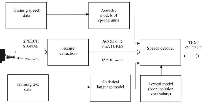
3.2 Automatic Speech Recognition (ASR):

Figure 1. Components in an ASR system.

This section describes the parts of a traditional ASR system. A general ASR system has four main components: 1) Feature Extraction; 2) Acoustic Modeling; 3) Language Modeling; and 4) Lexical Modeling.

3.2.1 Feature Extraction

The front-end of any ASR system is the feature extraction phase, which takes as input the audio signal, and outputs the digital representation of the audio signal. Raw audio can be directly given as input to the ASR system, or it can be converted to the frequency domain, and either passed as spectrograms, or a feature extraction technique can be applied on the frequency domain representation of the audio signal. Various feature extraction techniques include: Mel Frequency Cepstral Coefficients (MFCC), Linear Prediction Coefficients (LPC), Perceptual Linear

Training speech

data models of Acoustic

speech units Training Speech Data

Feature

extraction Speech decoder

Training text data

Statistical

language model _{(pronunciation} Lexical model vocabulary) SPEECH SIGNAL W = w1,….wn ACOUSTIC FEATURES O = o1,….or TEXT OUTPUT

10

Prediction Coefficients (PLP), and bottleneck layer features (Multi-Layer Perceptron (MLP) outputs, specifically using autoencoders) etc.

3.2.2 Acoustic Modeling

An Acoustic Model (AM) is used in ASR to represent the relationship between an audio signal and the corresponding phonemes, characters, or words. AMs build statistical representations of meaningful speech units based on its input. Traditionally, ASR models were built using Hidden Markov Models (HMM). The most basic form was where each phoneme was modeled using separate HMMs, and the probabilities of the HMM were modeled using Gaussian Mixture Models (GMM). More recent approaches model the feature extraction, acoustic model and phoneme decoding system into the same end-to-end deep network. The acoustic model is specific to the language that is being modeled, as the phonemes differ from language-to-language. The acoustic model can however, be generalized over different accents of the same language using speaker normalization techniques.

3.2.3 Language Modeling

Once the acoustic model outputs the sequence of phonemes/characters/words corresponding to the input utterance, the language model makes corrections based upon prior probabilistic statistics. The Language Model (LM) is a probability distribution over a set of words, describing the probability of sounds/characters/words occurring together in sequence. The language model, like the acoustic model, is generally collected on large written corpus, which is independent of the acoustical corpus, and dependent on the language being modeled. The sequence probabilities differ immensely from language-to-language.

11

3.2.4 Lexical Modeling

The Lexical Model (Dictionary) plays a crucial role in any ASR system, as it acts as a bridge between the audio based acoustic model and the text-based language model. The lexicon has a two-fold role to play in an ASR system: 1) It contains the list of all words that can possibly be recognized by the ASR model, and 2) It helps traditional HMM models in building decoder models for each phoneme. The dictionary has two parts to it: 1) the words that the ASR system can recognize; and 2) the phoneme composition to produce the words. It is often crucial to include all possible words and phonemes in a language in the lexicon to obtain good performance of the ASR system.

3.3 Mel Frequency Cepstral Coefficients (MFCC)

The Mel Frequency Cepstral Coefficient (MFCC) is a popular feature representation method used for speech signals. It is based on the concept of Cepstrum, which represents the power of a signal. The steps involved in calculating the MFCCs of a speech signal are as follows:

3.3.1 Pre-emphasis:

The first step in the MFCC feature extraction process is to increase the energy content of the signal in the high frequencies. This is performed as the spectrum (the spectrum of the waveform is the summation of sinusoids, each with a particular amplitude and phase) for voiced segments has less energy at higher frequencies than at lower frequency. This is called a Spectral tilt. Sounds like [r], [g], [j], and [b] are voiced and sounds like [s], [p], [k] and [t] are unvoiced. The main difference between the two are, in voiced sounds the vocal folds vibrate, and in unvoiced sounds they don’t. They are mostly uttered from the front end of the vocal tract. Boosting high-frequency energy gives more information to the acoustic model. This helps in improving phone recognition performance.

12

3.3.2 Windowing:

Speech is an aperiodic signal and its properties change with time. Therefore, information is extracted from a small enough signal region where the speech signal seems relatively stationary, improving the spectral information for phone recognition. However, when computing the Discrete Fourier Transform (DFT), it assumes that the small signal region is one period of a continuous periodic signal. In the case of speech signals, the aperiodic nature may cause discontinuities. These discontinuities can affect the spectrum by showing up as high frequency components which don’t appear in the original signal. These effects can be minimized using a technique called windowing. Windowing suppresses the amplitude of these discontinuities that occur at the boundaries of each signal region. It is usually done using the Hamming window, as it performs better than rectangular window in the calculation of MFCCs. Hamming window causes the side lobes to be suppressed significantly compared to the main lobe making the results cleaner and better suited for frequency-selective analysis.

3.3.3 Discrete Fourier Transform:

We then extract spectral information from the windowed signals using Discrete Fourier Transform to obtain the energy of the signal at different frequency bands.

3.3.4 Mel Filter Bank and Log:

Human hearing is not uniformly sensitive to all frequency bands. It is more sensitive to lower frequencies than to higher frequencies. This property can be modeled using mel-scale. A mel is a unit of pitch [24]. The mel-scale is more closely related to human hearing than a time-frequency domain representation like the spectrogram, as human perception of time-frequency is more non-linear than linear. As mentioned in section 3.3.1, the mel-scale performs pre-emphasis on higher frequencies, which is not performed while constructing the spectrogram.Finally, the log

13

levels of each of the mel spectrum values are computed. Logarithmic scaling compresses higher frequencies.

3.3.5 The Cepstrum:

Speech is created by the glottal source output being passed through the vocal tract, which has a filtering characteristic because of its ability to form various shapes [24]. The cepstrum is used to separate the glottal source from the filter. For phone detection, it is more important to extract details on the vocal tract filtering than the glottal source output. The cepstrum is calculated by finding the inverse DFT of the Mel filter bank output.

A typical cepstrum has a large peak at the fundamental frequency F0 which represents the glottal pulse, and higher harmonic components at lower amplitudes which represent the vocal tract filters. By using the cepstrum values between the second and the thirteenth peak and ignoring the fundamental frequency peak, we can separate the source from the filter.

Cepstral coefficients do not capture the energy information. So, we add an energy feature to it. The energy of samples in any given frame is the sum of the squares of the samples over time [24]. Consider a signal x, which is windowed from time t1 to t2. The energy for this signal can be

found as: 𝐸 = $ 𝑥(𝑖)) *) (1)

Speech signals are not constant as the slope of formants changes from stop burst to release. So, we want to add these variations in the features. For each of the 13 cesptral values, a delta or

14

velocity value is added. The delta values correspond to a change between frames in the corresponding cepstral/energy feature. It can be calculated as:

𝑑(𝑡) =𝑐(𝑡 + 1) − 𝑐(𝑡 − 1)

2 (2)

Where d(t) represents the delta value, and c(t) is the cepstral value at time t. Similarly, 13 double delta features are added, which correspond to the change between frames in the corresponding delta values.

3.4 The Deep Speech model

Deep Speech is an ASR system developed by Baidu research. It focuses on making an end-to-end ASR deep learning system. The architecture combines various parts of the complex ASR pipeline to make a simpler pipeline. These end-to-end pipelines are more robust to noisy speech, combining the pre-processing step, the acoustic model and the decoder. Unlike traditional ASR systems, Deep Speech does not model noise, reverberation, or speaker variation using hand-crafted methods. Raw spectrogram data is fed into the model and it directly learns to compensate for these effects. The paper experiments with noise addition as a method of data augmentation. The input method is spectrograms sampled at 16 kHz and output is at character level, which is then corrected using a separately trained language model. The model is a five-layer recurrent neural network, where the first three layers as well as the last layer are non-recurrent, while the fourth layer is bidirectional recurrent. Each layer contains 2048 hidden units per layer. The model is trained on 12000 hours of English data, comprising various types of datasets (conversational as well as read).

15

16

Chapter 4

Generative Adversarial Networks

4.1 Generative Adversarial Networks Preliminaries

Generative Adversarial Networks (GANs) are generative models introduced by Goodfellow et al. [1]. The framework comprises of a combination of two neural networks, a generator and a discriminator, each with different roles, going against one another to generate real looking images from a distribution that it is trained on. The generator tries to generate images that resemble images from a real distribution of one particular class. The role of the discriminator is to classify the images as being a real (an image from the real distribution of images of the class) or a fake image (an image generated by the generator which resembles the characteristics of an image from the real distribution). The generator and the discriminator are trained together, with the generator getting better every iteration at generating real looking images that fool the discriminator; and the discriminator getting better every iteration at discerning between real and fake images. When we get to the point where both the generator and discriminator feel they are at an optimal training position, we call that Nash equilibrium.

GANs belong to the class of models called generative models. There are two broad kinds of machine learning models: Generative models and Discriminative models. Discriminative models, like Support Vector Machines, learn decision boundaries from the data. Generative models on the other hand learn the intrinsic probability distributions from the given data. Generative models used in GANs, use input space probability distributions to generate synthetic input samples.

17

4.2 CycleGAN

Image-to-Image translation is a method that transforms images from one distribution of images to another without changing the background features, i.e., the other features in the images that do not pertain to either domain are kept recognizably the same. The barrier for this application however, is that there is a dearth of datasets that contain paired images, i.e., an (X,Y) pair of images, where X is a sample from distribution A and Y is a sample from distribution B, that correspond to a 1:1 mapping between the two images with all features remaining the same except the distinguishing feature that discriminates between the two domains. This can be overcome by developing methods that can transform images from one domain to another without the need for paired images.

Figure 3. Image of domain transformation of images using CycleGAN [18]. (Reproduced without permission)

CycleGAN [18] performs unpaired image-to-image translation, i.e., image translation without the need for (X,Y) paired images. The advantage of CycleGAN lies in being able to learn transformations without a one-to-one mapping between training data in source and target domains. CycleGAN eliminates the need for paired images by first transforming the image into

18

the target domain, and then transforming the target image back into the source domain. A cycle-consistency loss is introduced to drive the network to such a behavior, such that transforming a particular image from the source domain to the target domain and back, reproduces the same sample from the source domain, to ensure that the structure of the object (in the image) being transformed is retained, and only the distinguishing features are changed.

Figure 4. Data flow in CycleGAN [18]. (Reproduced without permission)

CycleGAN uses two generators and two discriminators to be able to translate between the two domains. Consider two domains, A and B.One generator transforms from domain A to domain

B, say G, and the other transforms from domain B to domain A, say F. Each generator has a corresponding discriminator, which is responsible for determining if it is receiving a real image in the domain from the dataset, or a fake one being generated by the generator.

The way CycleGANs are able to learn translations without having explicit A/B training images involves introducing the idea of a full translation cycle to determine how good the entire translation system is, thus improving both generators at the same time. In a nutshell, consider an image I1 from domain A. This image is passed through a generator, G, which transforms this

19

generator, F, which converts the image back to domain A from domain B, I1cyclic. The aim is to

minimize the distance between the latent representation of I1 and I1cyclic.

Figure 5. Full translation cycle in CycleGAN [18]. (Reproduced without permission)

4.3 DiscoGAN and Difference between CycleGAN and DiscoGAN

Kim et. al [25] performed similar research in unpaired image-to-image translation. However, the focus of this paper involved transforming patterns from an object of one domain, to the object of another. For example, transferring the patterns on a bag onto a shoe. DiscoGAN and CycleGAN have very similar network architectures. DiscoGAN also has a pair of GANs that map data from one domain to another and back. A reconstruction loss is used to measure the reconstruction accuracy of the original image after the two transformations. The two papers use the original formulation of the loss function of GANs as their basis for the loss function for the style transfer GAN.

However, the differences between the two networks lies in the fact that DiscoGAN uses two reconstruction loss computations, one for each GAN, while CycleGAN uses one cycle-consistency loss.

20

4.4 VoiceGAN

Voice impersonation is a complex phenomenon that involves producing a target voice that convincingly represents the impression of naturally having been produced by the target speaker. It is usually aimed at mimicking the pitch among many other perceivable signal properties and is not the only transient factor.

Consider the case where a human impersonator learns to mimic the voice of another person. In most cases, the source impersonator learns to mimic elements such as the voice quality of the target speaker. This is however a hard-to-measure aspect, and is often characterized by nasality, roughness etc., and these aspects allow measurable comparisons between speakers.

VoiceGAN aims to achieve automatic generation of impersonations by style transfer between two speakers. Many conventional methods of voice transformation modify the instantaneous characteristics of a given signal. While these methods are effective, they fall short in being able to capture unmeasurable and unquantifiable elements of voice. They are also heavily reliant on parallel recordings of the source and target speakers.

4.4.1 Image vs Speech samples

Before going into voice impersonation by generation, it is useful to look at some of the fundamental differences between image and speech datasets.

1. Unlike images, speech samples vary in length across the dataset, i.e. they are not fixed in duration of sample. Speech samples generally cannot be scaled to have the same duration, as resampling may affect stylistic features.

21

2. Generation of time-series data like speech is far from straight-forward when compared to images. Naïve implementations may result in loss of linguistic, stylistic or even intelligible content.

4.4.2 VoiceGAN model changes

VoiceGAN is an extension of DiscoGAN, which was designed to perform style transfer in the image domain. To be able to apply a DiscoGAN on speech data, the data must be pre-processed to a picture-like representation. DiscoGAN does this by utilizing spectrograms. Some of the changes that were made to the architecture of DiscoGAN to be able to perform style transfer on speech data are detailed below.

4.4.2.1 Retaining linguistic information

Linguistic information is contained mainly in the spectral envelope of samples, and this must be retained to be able to reconstruct the speech sample and maintain the linguistic content. For this, the reconstruction loss was modified as:

𝐿constA=a𝑑(𝑥ABA, 𝑥A) + b𝑑(𝑥AB, 𝑥A) (3)

The term d(xAB, xA) attempts to retain the linguistic information in the intermediate states

as well, and d(xABA, xA) attempts to retain the linguistic information after the reconstruction has

22

4.4.2.2 Variable-length input generator and discriminator

As mentioned before, speech data unlike image data, isn’t of a fixed size. The architecture of DiscoGAN must also be altered to handle this variable-length input. In DiscoGAN, the generator contains a fully convolutional layer between the encoder and decoder, and this can be used as a mechanism to handle variable-length input, and hence the generator does not need to be modified. The discriminator, however, requires a modification. The max-pooling performed in the discriminator of DiscoGAN is replaced with an adaptive pooling layer in VoiceGAN, as shown below.

a) Generator of VoiceGAN b) Discriminator of VoiceGAN Figure 6. Generator and Discriminator of VoiceGAN [17]. (Reproduced without permission)

4.4.2.3 Style Embedding Model

A second discriminator was also added to discriminate between style information in the input data to ensure that the style information is contained in the generated sample. This introduces a new component into the loss function as follows.

LDSTYLE-A = d(DS(xA), labelA) + d(DS(xAB), labelB) + d(DS(xABA), labelA) (4)

LDSTYLE = LDSTYLE-A + LDSTYLE-B (5)

Therefore, the total discriminator loss becomes,

23

4.5 StarGAN – VC

While VoiceGAN [17] converts speech samples from one speaker to another using non-parallel data, two limitations of the VoiceGAN network are, 1) the network takes inputs as single-frames; and 2) it creates one-to-one mappings between classes. StarGAN-VC [26], a voice conversion network derived from the StarGAN, helps overcome these two limitations by being able to create many-to-many mappings, using just one generator G to convert samples between categories, and being able to process inputs as feature sequences instead of single-frames, by modifying the Generator CNN to be fully convolutional.

The discriminator as well as domain classifier are designed in such a way that they classify segments of the sequences, instead of the whole sequence. They leverage the idea of PatchGAN [27], which classifies whether local segments of input sequences are real or fake. The objective function used to train the StarGAN-VC model is described below.

4.5.1 Objectives

24

Figure 8. StarGAN-VC [26]. (Reproduced without permission)

Figure 7, shows the network for voice conversion that is derived from CycleGAN. The input to the network is the VCC 2016 dataset, with one male and one female speaker. The utterances are divided into 216 short parallel sentences. CycleGAN-VC uses a cycle-consistency adversarial network, along with a gated convolutional neural network (CNN) as the generator. The adversarial loss in this case, helps in mitigating the smoothing effect created by the generator while converting between two classes. The CycleGAN is trained with an identity-mapping loss function. Figure 8, shows the StarGAN-VC voice conversion network. In this network, the generator G takes acoustic feature sequences as input. These feature sequences are a set of concatenated one-hot encoded vectors, that correspond to the speech attributes comprising of one or more classes. The discriminator network D, and the domain classifier C, are identical to that of VoiceGAN or CycleGAN-VC. The training objectives used to train the model are similar training objectives as in VoiceGAN.

25

4.5.1.1 Adversarial Loss

The adversarial loss is similar to the adversarial loss defined in [1], and is:

LADVD(D) = – Ec~p(c), y~p(y|c)[log(D(y,c))] – Ex~p(x), c~p(c)[log(1 - D(G(x,c),c))] (7)

LADVG(G) = – Ex~p(x), c~p(c)[log(D(G(x,c),c))] (8)

LADVD(D) is low when D correctly classifies the speech samples in the dataset as real and those

generated by G as fake. LADVG(G) is low when G is able to deceive D into thinking that the image

generated by G is real.

4.5.1.2 Domain Classification Loss

The domain classification loss takes care of checking which domain or category the output belongs to, and is:

LclsC(C) = – Ec~p(c), y~p(y|c)[log(pC(c|y))] (9)

LclsG(G) = – Ex~p(x), c~p(c)[log(pC(c|G(x,c)))] (10)

The above two equations are low when they correctly classify the utterances as belonging to a certain class c.

4.5.1.3 Cycle Consistency Loss

Cycle Consistency loss maintains the linguistic information in the utterances, by reducing the distance between the converted sample and the original sample.

Lcyc(G) = E c’~p(c), x~p(x|c’), c~p(c))[||G(G(x,c),c’) – x||r] (11)

26

The final objective functions are:

ID(D) = LADVD(D) (13)

IC(C) = LclsC(C) (14)

ID(G) = LADVG(G) + lcls LclsG(G) + lcyc Lcyc(G) + lid Lid(G) (15)

ID(D) is low when D correctly classifies the speech samples in the dataset as real and those

generated by G as fake. IC(C) is the domain classification loss, and it checks and classifies the

samples input to their respective classes. This ensures that the samples being generated are similar to the ones in the input data distribution. The generator loss is a linear combination of the adversarial loss for generator, which is high when the generator can synthesize samples very similar to the distribution of the input data, the cycle consistency loss, and the identity mapping loss, which makes sure that the linguistic information between the input and the transformed output is the same.

4.6 StarGAN-VC v/s VoiceGAN

StarGAN-VC is derived from CycleGAN, which has one cycle-consistency loss, while VoiceGAN is derived from DiscoGAN which has two reconstruction losses. The advantage of having one combined loss over two separate losses is that, all the domains are mapped to one latent space, as opposed to multiple latent spaces. This has the advantage of performing many-to-many mappings, and the sample size for each class need not be very large. Another advantage of StarGAN-VC over VoiceGAN is that, the discriminator is borrowed from PatchGAN, which classifies patches of the output spectrogram as real or fake, as opposed to the whole sample. This has the added advantage of processing different lengths of samples. Therefore, there is no cropping that has to be performed for the voice samples, and this eliminates any artifacts that arise when combining cropped samples back together into one speech sample.

27

Chapter 5

Raw audio, spectrograms and MFCCs

A spectrogram is a basic input method in audio analysis and other applications. It is an important representation of audio data as human hearing is based on a real-time spectrogram. The spectrogram is a popular choice of audio representation used in the development of sound synthesis algorithms. Spectrograms are useful in synthesis models when trying to approximate time-domain representation of signals based on their frequency domain representation, as matching the spectrogram often corresponds to matching the sound extremely well.

This chapter focuses on understanding raw audio, spectrograms, MFCCs and how to convert to and from one type of input method to another. This is often useful when using generative modeling methods such as Generative Adversarial Networks (GANs) [1] for various applications.

5.1 What is the raw audio format?

The raw audio format is an audio file format that contains uncompressed audio in the raw form. The samples represent the amplitude values of the speech signal with respect to time.

5.2 What are spectrograms?

Like many real-world signals, speech signals vary over time. While performing spectral analysis on speech signals, it is often assumed that the signal frequency content is stationary only over a short period of time. To be able to extend this analysis to longer signals, we need to be able to combine analysis over a series of short time slots. A spectrogram is built from a sequence of frequency spectrums, by stacking them together in time.

28

Spectrograms are visual representations of signal strength over time at various frequencies present in a particular speech sample. Spectrograms are two dimensional graphs, with the two dimensions being time on the horizontal axis and frequency on the vertical axis.

5.2.1 Wideband and Narrowband spectrograms

There are two broad categories of spectrograms that can be calculated based on the range of the pass band frequencies of the sampling filter applied to the raw audio signal. If the sampling bandpass filter is of short duration (~300Hz) the spectrogram is said to have a wide bandwidth and displays good temporal resolution, but poor frequency resolution. On the other hand, if the sampling bandpass filter is of long duration (~45Hz), the spectrogram is said to have narrow bandwidth and has good frequency resolution, but poor time resolution.

29

Figure 9. Wideband spectrogram. [29] (Looks like good frequency, but quantized time) (Reproduced without permission)

Figure 10. Narrowband spectrogram. [29] (Looks like poor frequency, but good time) (Reproduced without permission)

30

In Figures 9 and 10, the top row of Figure 9 has speech signals windowed using a window size of short duration (~3ms). Due to the size of the window, the waveform can be thought of as representing one period of the full sample. The top row of Figure 10 has speech signals windowed using a window size of longer duration (~20ms). Due to the size of the window, the waveform can be thought of as representing the entire sample.

In Figures 9 and 10, the signal on the top row in both figures correspond to the waveform of the speech signal in time domain. The bottom row in Figure 9 corresponds to the wideband spectrogram of the signal (using a bandwidth of 300Hz), where the temporal information, i.e., the individual vocal fold pulses can be seen clearly. The bottom row in Figure 10 corresponds to the narrowband spectrogram of the signal (using a bandwidth of 45Hz), where the frequency resolution, i.e., the individual formant information at each timeslot can be seen clearly.

5.3 Computing the spectrogram

Consider a signal ‘x’ of length N samples. To calculate the spectrogram of this signal, it is first split into overlapping segments of length M where M < N. The Fourier transform of each of the segments is computed and stacked together in time to obtain the spectrogram.

The parameters required for calculating the spectrogram of a signal are:

1. The FFT size that needs to be used for each frame – a common choice of FFT size is a value which is a power of 2 (e.g. = 512).

2. The sampling frequency of the signal – a common choice of sampling frequency is 8 kHz. 3. The window length to compute the FFT of each frame of the signal – a common choice for window length is 20ms. This is short enough for the window to contain typically only one phoneme. (Note: The spectrogram of a signal is calculated as a stacked spectrum of many segments of the signal, where each of these segments represent a frame. The segments are

31

processed using the conventional FFT algorithm, which performs windowing of the signal to isolate the phonemes)

4. Number of samples of overlap – typically at least 50% overlap.

5. Window type – usually chosen to be Hamming, due to its property of being able to attenuate the sidelobes, making it better suited for frequency selective analysis.

Typical spectrograms show log-magnitude intensity (dB) of the frequency signal versus linear time. This is useful as the human hear perceives changes in frequency logarithmically at higher frequencies, as compared to lower frequencies where they are perceived linearly, and this is reasonably well modelled by spectrograms.

5.3.1 Input values to Deep Speech

The input to the Deep Speech model are MFCCs, with the following parameters: 1. Window length = 25msec

2. Window step = 10msec (which makes overlap of 15msec)

3. Number of Cepstral coefficients being used = 13 (+ 12 delta features and 1 energy feature + 12 double delta features and 1 energy feature; as described in chapter 3.)

4. FFT size = 512

5. Sampling rate = 16 kHz

6. Window type = Hamming window

5.4 Converting spectrogram to raw audio

The spectrogram of a waveform represents the magnitude distribution of the Fourier transform of the signal. While there is some phase information inherently retained in the spectrogram, a lot of the information is lost. The phase information plays a crucial role in being able to reconstruct a signal effectively. But with lost information, a good way of obtaining the

32

time domain representation of the signal is to find a signal whose Short Time Fourier Transform (STFT) is close to the STFT of the signal that was originally used to construct the spectrogram.

Consider a signal xn, which needs to be reconstructed from its spectrogram. Let X(mS, ω)

represent its STFT, where S is the sampling frequency, ω is the frequency (= 2πf) and m is the current time. Let the window used for STFT be denoted by w(n), which is of length L. By definition STFT is,

𝑋(𝑚𝑆, 𝜔) = 𝐹[𝑥(𝑚𝑆, 𝑙)] = $ 𝑥(𝑚𝑆, 𝑙)𝑒@+A* ₍₁₆₎ C

D, @C

Where, x(mS, l) = w(mS – l) * xn and 𝐹[𝑥(𝑚𝑆, 𝑙)] represents the Fourier transform of x(mS, l).

Consider an arbitrary STFT, Y(mS, ω), which denotes the STFT of y(mS, l), where,

𝑦(𝑚𝑆, 𝑙) = 1

2𝜋G 𝑌(𝑚𝑆, 𝜔)𝑒+A*𝑑𝜔 (17)

J A, @J

𝑌(𝑚𝑆, 𝜔) can be obtained by minimizing the distance between X(mS, ω) and 𝑌(𝑚𝑆, 𝜔), using the following formula,

𝐷[𝑥(𝑛), 𝑌(𝑚𝑆, 𝜔)] = $ 1 2𝜋 G |𝑋(𝑚𝑆, 𝜔) − 𝑌(𝑚𝑆, 𝜔)|) 𝑑𝜔 (18) J A, @J C O, @C

This squared error between X(mS, ω) and 𝑌(𝑚𝑆, 𝜔) is decreased at each iteration to obtain the reconstructed signal. The authors in [30] solve this equation using Parseval’s theorem and by setting the gradient w.r.t x(n) to 0. The result is,

𝑥(𝑛) =∑CO, @C_∑ 𝑤(𝑚𝑆 − 𝑛)𝑦(𝑚𝑆, 𝑛) 𝑤)_{(𝑚𝑆 − 𝑛)} C

33

The i+1st _{estimate of x}i+1_{(n) is obtained by taking the STFT of x}i_{(n), by replacing the magnitude}

of Xi_{(mS,w) with the magnitude of Y(mS, w), and then finding the signal whose STFT is closest}

to the modified STFT.

5.5 Computing MFCCs from a spectrogram

One method to compute MFCCs from a spectrogram would be to go from spectrogram to raw audio and then compute the MFCCs from the raw audio. But as a spectrogram is already in the frequency domain, it is possible to go directly from spectrograms to MFCCs, without the intermediate step of going into the time domain.

We start with the output of DFT, and calculate the log levels of each of the spectrum values using the following formula,

𝑀(𝑓) = 1125 ∗ 𝑙 𝑛 W1 + 𝑓

700Y (20)

Where, M(f) is the mel spectrum value of frequency value f.

The next step is to take the inverse DFT of mel filter bank output, which is called the cepstrum. Use the cepstrum values between the second and the thirteenth peak ignoring the fundamental frequency peak. Add the energy feature to it. The energy of samples in any given frame is the sum of the squares of the samples over time. Finally, add the delta and double delta features.

34

Chapter 6

Thesis Proposal

6.1 Problem Statement

The aim of this thesis is to examine the effect of different augmentation techniques and to examine the effectiveness of GANs in voice transformation and its limitations. Various speech data augmentation techniques such as noise augmentation, pitch augmentation as well as speed augmentation will be experimented with. Each will be analyzed under different conditions using different control variables, to determine which of the augmentation techniques works well for the dataset, and which of them don’t. Voice conversion as an augmentation technique can also be used improve the robustness of a speech recognition model to a dataset. The information gained from the study on the limitations of GANs in the field of voice conversion will aid this research further in collection of data, specifically, in understanding the conditions required for the data to be collected in, so that the GAN can effectively perform voice transformation.

6.2 Datasets

6.2.1 Seneca dataset

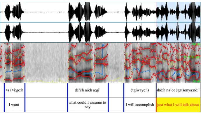
The Seneca dataset is a 315-minute corpus of natural conversation American Indian Seneca. 270 minutes of annotated audio data are used for training and randomly selected 45 minutes of annotated audio data are used for testing. The dataset was annotated and aligned using Praat [31]. The dataset was recorded as long conversations between two speakers. An utterance is considered as one sentence spoken by each speaker. Every sample, which consists of multiple sentences, is broken down into utterances (or single sentence samples), and the annotation is done at the utterance level. In Figure 11, the top row represents the speech signal waveform. The second row is the spectrogram representing the speech signal with the red dots representing the formants,

35

the yellow line representing the intensity of the signal and the blue line representing the pitch of the signal. The last row represents the annotation of each utterance.

The lexicon consists of 3,498 Seneca words. The corpus used to create the language model consists of 1,843 utterances that consists of transcribed data as well as text found online, such as Seneca to English dictionaries that could be used as input to create the language model.

The Deep Speech model requires csv files as inputs which contain the file name and file path, the file size and the transcription. The audio files are required to be in .wav format. Code was written to compile the audio file paths, size and transcription into a csv file, as well as to convert the audio files into .wav format.

36

6.2.2 Free Spoken Digits dataset

The free-spoken digits dataset [32] is a corpus of three speakers uttering the words zero through nine, with each speaker uttering each word 50 times. Overall, the dataset contains 1500 utterances of zero through nine by three speakers. The utterances are recorded at 8 kHz sampling frequency, which is often characteristic of cellphone microphones. The lexicon for the dataset is 10 words, zero through nine. The utterances are less than a second long.

Of the three speakers, two were chosen as the two domains. The dataset was split 90:10 train to test split.

6.2.3 LibriSpeech

The LibriSpeech corpus [33] is an English dataset of approximately 1000 hours of English being read. The dataset was developed by Daniel Povey and Vassil Panayotov. The dataset is part of the audiobooks from LibriVox project. The utterances are sampled at 16 kHz sampling frequency. The utterances range between 12-20 seconds long.

6.2.4 Tensorflow Speech Recognition Challenge Dataset

The Tensorflow Speech Recognition Challenge Dataset [34] contains 65,000 one second long utterances of 30 short-words such as ‘right’, ‘left’, ‘go’, ‘stop’, ‘one’, ‘two’ and so on, spoken by thousands of people. The utterances are sampled at 16 kHz sampling frequency. Each class of utterance contains thousands of samples of men and women speaking the word. Each utterance in this dataset is just one word.

37

6.2.5 Voice Conversion Challenge 2018 Parallel Dataset

The Voice Conversion Challenge 2018 dataset [35] is a challenge for voice conversion, i.e., converting the utterance of a source speaker to that of a target speaker without changing the content of what was spoken. It contains synchronous data, i.e., both speakers speaking the same utterances. It has two male and two female speakers with 81 utterances of each speaker. The utterances are sampled at 22 kHz. The utterances range between 4-5 seconds long.

6.3 Language Model

The language model file, ‘lm.binary’ file was created using the KenLM software [36]. The input to the software is the Seneca corpus, which is a text file that contains the transcribed utterances and other Seneca data from the internet, including the Seneca to English dictionary. The data is organized as one utterance per line. KenLM evaluates and prunes language models with modified Kneser-Ney smoothing algorithm [37]. KenLM offers two data structures: Probing and Trie. Probing is the default setting on the software and is the faster of the two, while the trie data structure uses the least memory, has the best memory locality and is fairly fast. The trie data structure takes longer to build than probing.

6.4 Data Augmentation

6.4.1 Noise Addition

The simplest form of data augmentation used for speech signals is adding noise to the speech signal at a given signal-to-noise ratio (SNR). Noise addition to a speech signal can be done several ways. Two popular methods are:

a. Generate a random vector (of normal distribution) of length equal to the speech wave. This vector of random numbers can then be added to the speech signal.

38

When using this method, it is important that the start time of the noise file is random. This prevents regular and predictable sounds such as a door banging or a guy laughing at the same point in every file. The noise signal must be scaled using a signal-to-noise ratio that provides maximum intelligibility. The procedure is described below.

Consider a speech signal sampled at frequency fs Hz, with samples S = {s1, s2, s3, …, sn},

and a noise signal sampled at frequency fs Hz, with samples N = {n1, n2, n3, …, nn}, where N is the

total number of samples in the signal, while ni is the ith sample of the signal. The number of

samples, the length of the two signals, and the sampling frequency must be the same to add the two signals. The SNR in this case would be,

𝑆𝑁𝑅 = 10𝑙𝑜𝑔-^ 𝐸𝑠𝑝𝑒𝑒𝑐ℎ 𝐸𝑛𝑜𝑖𝑠𝑒 (21) where, 𝐸𝑠𝑝𝑒𝑒𝑐ℎ = $ 𝑠(𝑖)) b +,^ (22) and 𝐸𝑛𝑜𝑖𝑠𝑒 = $ 𝑛(𝑖)) b +,^ (23)

Where ESpeech and ENoise are the energies of the speech signal and the noise signal

respectively. Upon choosing the required SNR, the scaling factor K, for the noise signal can be calculated as,

𝐾 = e𝐸𝑆𝑝𝑒𝑒𝑐ℎ 10fbg(hi)-^

39

Where ESpeech is the energy of the speech signal and SNR (dB) is the required SNR. Once

the scaling factor K has been found using (11), with Espeech from (9) and a chosen SNR value (the SNR value is chosen such that the speech content is understandable even after being augmented by adding noise), the speech samples and the scaled noise samples can be added together to get the new augmented signal:

𝑥(𝑖) = 𝑠(𝑖) + (𝐾 ∗ 𝑛(𝑖)) (25) Where x(i) is the samples of the new signal, s(i) is the speech signal samples and 𝑛^(𝑖) is the scaled noise signal samples.

6.4.2 Pitch Augmentation

Pitch is defined as the rate at which the vocal folds vibrate. There could be various other reasons for change in pitch including thickness of the vocal folds and change in emotion such as anger or excitement, but the rate of vibration of vocal folds is the most influential.

Pitch augmentation involves raising or lowering the pitch of the audio sample by resampling the audio file. The file is resampled in octaves. Increasing the pitch by half an octave increases the speed of the speech sample proportionally as well. The sampling rate fs can be

mapped to a new sampling rate fs’ using (8),

𝑓𝑠l _{= 𝑓𝑠 ∗ 2}m ₍₂₆₎

Where x is a randomly chosen pitch shift in octaves. For example, a shift in the pitch of

the speech sample sampled at 16000 Hz by half an octave (tritone) is 16000 Hz * 2^.o _{~ 22600 Hz.}

The new sampling rate for the given speech sample is set as 22.6 kHz. As the number of samples remain the same but are played back at a higher sampling rate, the speed of the speech sample increases with the pitch. The speech sample is then resampled at the original sampling rate of 16 kHz. This method of pitch shifting is called the chipmunk method of pitch shifting.

40

6.4.3 Speed Augmentation

Speed augmentation involves changing the speed of playback of the speech sample to a higher or lower speed. The speed of the speech sample can be increased by resampling the utterance at a higher or lower sampling frequency.

6.5 Research Questions

The research questions that will be the focus of this thesis are:

• Does transfer learning on a pre-trained model help improve a model's robustness towards resource constrained languages?

• Does sample augmentation help improve the model's robustness and result in lower Word Error Rate (WER)?

• Which augmentation technique, among the ones being used (noise addition, pitch, speed, voice conversion), is optimal in making the ASR model more robust towards Seneca? • Which of the current Generative Adversarial Network (GAN) technologies is best for

voice conversion?