atmospheres using comprehensive two
dimensional gas chromatography
Rachel Ellen Dunmore
Doctor of Philosophy
University of York Chemistry
To all the people who made this possible. You know who you are.
”An education isn’t how much you have committed to memory, or even how much you know. It’s being able to differentiate between
what you know and what you don’t.”
Volatile organic compounds (VOCs) are key precursors to ozone and particulate matter,
two of the most important air pollutants. Air quality interventions have successfully
reduced the release of short chain VOCs in urban areas. The increased use of diesel vehicles has created an increase in the direct emission of longer chain VOCs. However, these compounds are not considered as part of air quality strategies and there are few atmospheric measurements of them to date.
This thesis details continuous measurements of VOCs in London, a developed megacity, using comprehensive two dimensional gas chromatography. Analysis of this large suite of VOC measurements have shown that the higher carbon number species emitted from diesel vehicles can dominate gas phase reactive carbon in cities with a significant diesel fleet. Comparison of these real-world observations with emissions inventories has highlighted that there is a significant under prediction of the emissions of higher carbon number species. This presents a considerable policy challenge; the focus must now switch to VOCs released from diesel as this vehicle type is increasingly replacing gasoline world-wide.
Further analysis of the London data has provided evidence of both anthropogenic and biogenic emission sources. The measurement of the higher carbon number species has allowed for OH reactivity to be more accurately modelled. Detailed analysis of the ethanol observations provided direct evidence that the use of bio-ethanol blended gasoline in the UK is having an impact on the composition of the atmosphere.
The combination of heart-cut and comprehensive two dimensional gas chromatography into a single instrument has made the measurement of both small and large chain VOCs possible. This instrument compares well to existing instrumentation and when deployed to a rural location (Bachok, Malaysia) provided hourly time-resolved measurements of C5-C13 VOCs.
Abstract 3
List of figures 9
List of tables 16
Acknowledgements 19
Declaration 21
1 The role of volatile organic compounds in urban air quality 23
1.1 Air quality . . . 24
1.1.1 Health effects of air pollution . . . 26
1.1.2 Climate effects of air pollution . . . 28
1.1.3 Air quality and climate change . . . 31
1.2 Volatile organic compounds . . . 32
1.2.1 Emission sources of volatile organic compounds . . . 34
1.2.1.1 Anthropogenic sources . . . 35
1.2.1.2 Biogenic sources . . . 35
1.2.2 Chemistry of volatile organic compounds . . . 36
1.2.2.1 Reaction of volatile organic compounds with radicals . . . 37
1.2.3 Formation of ozone . . . 41
1.2.4 Particulate matter in urban areas . . . 44
1.3 Measurements of volatile organic compounds . . . 45
1.3.1 Gas chromatography . . . 46
1.3.2 Comprehensive two-dimensional gas chromatography . . . 48
1.3.2.2 Orthogonality . . . 49 1.3.2.3 Data visualisation . . . 50 1.3.2.4 Ordered chromatograms . . . 50 1.3.3 Modulators . . . 51 1.3.3.1 Thermal modulators . . . 51 1.3.3.2 Cryogenic modulators . . . 54 1.3.3.3 Valve modulators . . . 55 1.4 Thesis outline . . . 57
2 Diesel-related hydrocarbons can dominate gas phase reactive carbon in megacities 59 2.1 Introduction . . . 60
2.1.1 Air quality in London . . . 64
2.2 Clean Air for London campaign . . . 64
2.2.1 Campaign sites . . . 65
2.2.2 Intensive operating periods . . . 65
2.3 Experimental . . . 66
2.3.1 Gas chromatography measurements . . . 66
2.3.1.1 Calibrations and uncertainties . . . 68
2.3.1.2 Liquid injections . . . 68
2.3.2 Supporting measurements . . . 70
2.4 Meteorology observations . . . 72
2.5 Observations of hydrocarbons in urban air . . . 75
2.5.1 Grouping of unresolved complex mixtures . . . 79
2.5.2 Seasonal behaviour . . . 81
2.5.3 Diurnal behaviour . . . 81
2.5.3.1 Impact of local meteorology in winter . . . 82
2.5.4 Comparison between London and Los Angeles . . . 84
2.5.4.1 Weekday vs.weekend . . . 85
2.5.5 Reactivity and mass calculations of grouped compounds . . . 86
2.5.5.1 Calculation of unmeasured diesel emissions . . . 90
2.5.6 Comparison to inventories . . . 92
2.5.7 Ozone formation potentials . . . 93
2.6 Conclusion . . . 97
3 Trends in volatile organic compounds and their reactivity in London during ClearfLo 101 Part 1: Trends in volatile organic compounds . . . 102
3.1 Seasonal comparison of observed mixing ratio, primary hydrocarbon OH radical reactivity and potential ozone formation . . . 103
3.1.1 Saturated aliphatic compounds . . . 104
3.1.2 Unsaturated aliphatic compounds . . . 106
3.1.3 Aromatic compounds . . . 108
3.1.4 Grouped unresolved complex mixture species . . . 110
3.2 Air mass analysis . . . 112
3.2.1 Air mass history . . . 112
3.2.2 Air mass processing ratios . . . 114
3.3 Anthropogenic volatile organic compounds . . . 117
3.3.1 Correlations between anthropogenic volatile organic compounds . . . 118
3.4 Biogenic volatile organic compounds . . . 120
3.4.1 Correlations of biogenic volatile organic compounds . . . 121
3.4.2 Relationship of biogenic species with temperature . . . 123
Part 2: Impacts of additional volatile organic compounds on modelled OH radical reactivity . . . 125
3.5 Introduction . . . 126
3.6 Experimental . . . 127
3.6.1 OH reactivity observations . . . 127
3.6.2 OH reactivity modelling . . . 127
3.6.3 Volatile organic compounds sets in the model . . . 128
3.7 Results . . . 130
3.7.1 Impact of using different sets of volatile organic compounds to cal-culate and model OH reactivity . . . 131
3.7.1.1 Standard and extended volatile organic compounds sets . . 132
3.7.1.2 Impact of model generated intermediates . . . 135
3.7.2 Impact of the grouped volatile organic compounds . . . 138
3.7.3 Influence of air mass origin on OH reactivity . . . 140
4 Investigating the magnitude and sources of oxygenated volatile organic
compounds in London during ClearfLo 143
Part 1: Analysis of oxygenated volatile organic compounds . . . 144
4.1 Seasonal comparison of oxygenated volatile organic compound observations 145 4.1.1 Diurnal profiles . . . 153
4.1.2 Direct anthropogenic emission of oxygenated volatile organic com-pounds . . . 157
4.1.3 Secondary oxygenated volatile organic compounds . . . 158
4.1.4 Other oxygenated volatile organic compounds . . . 159
Part 2: Atmospheric ethanol in London and the potential impacts of future fuel formulations . . . 161
4.2 Introduction . . . 162
4.3 Results . . . 166
4.3.1 Effect of ethanol content on acetaldehyde . . . 171
4.3.2 Impacts of ethanol blended fuel use on air quality . . . 173
4.3.2.1 Modelling using the Master Chemical Mechanism . . . 173
Conclusion . . . 176
5 Development of a combined heart-cut and comprehensive two dimen-sional gas chromatography system to extend the carbon range of volatile organic compounds analysis in a single instrument 178 5.1 Introduction . . . 179
5.1.1 Multidimensional gas chromatography . . . 181
5.1.1.1 Comprehensive two dimensional gas chromatography . . . 183
5.1.1.2 Hybrid gas chromatography systems . . . 184
5.1.2 Measurement of volatile organic compounds in rural atmospheres . . 187
5.2 Experimental . . . 190
5.2.1 Instrument comparisons . . . 190
5.2.2 Bachok demonstration ‘International Operating Fund’ campaign . . 190
5.3 Instrument design . . . 191
5.3.1 Cryo re-focussing step . . . 192
5.3.2 Instrument suitability . . . 194
5.3.3 Compound identification . . . 195
5.3.4 Intercomparison of two gas chromatography instruments . . . 199
5.4 Bachok demonstration campaign . . . 202
5.4.1 Time series . . . 205
5.4.2 Diurnal profiles . . . 206
5.4.3 Comparison to proton-transfer-reaction mass spectrometer . . . 208
5.5 Conclusion . . . 209
6 Conclusions and future work 211 A Correlations of individual and grouped volatile organic compounds 216 A.1 Winter correlations between volatile organic compounds . . . 217
A.2 Summer correlations between volatile organic compounds . . . 225
A.3 Correlations with oxygenated volatile organic compounds . . . 232
Abbreviations 243
1.1 Percentage of urban land use and city population for 1990 (top), 2014 (mid-dle) and predicted for 2030 (bottom) . . . 25
1.2 Summary of the key health effects associated with exposure to major
pol-lutants12,13 . . . 26
1.3 Radiative forcing estimates for 2011 relative to 1750 and aggregated
uncer-tainties for the main drivers of climate change28 . . . 29
1.4 Trade-offs from policies and technologies to tackle climate change and air
quality19,47–49 . . . 32
1.5 Gas-to-particle partitioning diagram of products from the reaction of O3
and α-pinene . . . 33
1.6 Simplified reaction cycle through which VOCs form O371 . . . 36
1.7 A simple schematic diagram through which the reactions of OH and HO2
radicals produce secondary pollutants76 . . . 37
1.8 Photochemical ozone formation as a function of the concentrations of VOCs
and NOx from vehicle exhaust emissions under different driving conditions.2 43
1.9 Typical EKMA diagram showing isopleths of 1-hr maximum ozone
concen-trations calculated as a function of initial VOC and NOx concentrations95,96 44
1.10 Illustration of the size of PM10 and PM2.5 particles in comparison to a
human hair and a grain of sand.97,98 . . . 45 1.11 Number of unique isomers possible as a function of the number of carbon
atoms in the molecule for alkanes and alcohols.103 . . . 46 1.12 Analysis of a Leeds urban air sample, with comparison of a single column
(upper) and GC×GC (lower) separation105 . . . 47
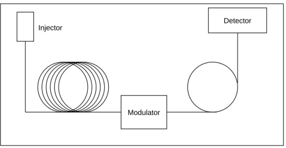
1.13 Typical GC×GC schematic showing the position of the modulation interface 48
1.14 Visualisation of how a GC×GC chromatogram is produced.116 . . . 51
1.16 Schematics of GC×GC setups with various modulators, (a) thermal (b) cryogenic and (c) valve119 . . . 53
1.17 Schematics of GC×GC valve modulators using open flow (a, upper panel)
and stopped flow (b, lower panel)131 . . . 56
2.1 Annual percentages of either new diesel car registrations or entire diesel car
fleet compositions for the EU, US and Japan over the last two decades.143 . 61
2.2 Total mass by carbon number and functionality from UK 2012 (left) and
US 2011 (right) emission inventories . . . 62
2.3 Isoprene and monoterpene annual flux for Great Britain in 1998.156 . . . . 63
2.4 Location of all ClearfLo sites, chosen for both long-term and intensive
mea-surements . . . 65
2.5 Location of the North Kensington site with possible VOC emission sources
highlighted . . . 66
2.6 GC×GC plots of the three different types of liquid injections . . . 71
2.7 Meteorological measurements of wind speed, temperature, solar radiation
and pressure from the winter and summer campaigns . . . 72
2.8 Campaign averaged wind rose plots for the winter (left) and summer (right)
campaigns . . . 73
2.9 Diurnal profiles of mixing layer height in winter (left-hand side) and summer
(right-hand side) . . . 74
2.10 Example correlations of the GC×GC-FID (x-axis) and the DC-GC-FID
(y-axis) instruments for n-hexane (left) and benzene (right) . . . 75
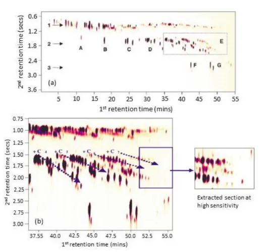
2.11 A typical GC×GC-FID plot from 2012-02-07 at 08:32 . . . 76
2.12 Typical GC×GC-FID chromatogram from 2012-07-25, demonstrating the
grouping of compounds . . . 80
2.13 Typical GC×GC-FID plot from the winter (upper; 2012-02-07 at 08:32)
and summer (lower; 2012-07-25 at 08:32) ClearfLo campaigns. . . 82
2.14 Diurnal profiles of selected urban pollutants in winter (left-hand side of each plot) and summer (right-hand side of each plot) . . . 83 2.15 Correlations of toluene and benzene measured during the winter campaign,
weekday (black) and weekend (red) . . . 86 2.16 Diurnal profiles of typically traffic source related compounds showing
2.17 Seasonal median values for hydrocarbon mixing ratio, mass concentration
and primary hydrocarbon OH radical reactivity in London . . . 90
2.18 Contributions of emission source to total mixing ratio, mass and OH radical reactivity for winter and summer . . . 91
2.19 Winter emissions inventory underestimation (left axis and blue columns) and the number of isomers included in each grouped set of compounds (right axis and black squares) . . . 93
2.20 Contribution of emission sources to potential ozone formation . . . 95
2.21 Potential SOA mass estimates . . . 97
2.22 Change in fuel use from 2005 to 2011178 . . . 99
3.1 Comparison of the contributions of the saturated aliphatic compounds to observed mixing ratio, calculated primary hydrocarbon OH reactivity and potential ozone formation . . . 105
3.2 Comparison of the contributions of the unsaturated aliphatic compounds to observed mixing ratio, calculated primary hydrocarbon OH reactivity and potential ozone formation . . . 107
3.3 Comparison of the contributions of the aromatic compounds to observed mixing ratio, calculated primary hydrocarbon OH reactivity and potential ozone formation . . . 109
3.4 Comparison of the contributions of the grouped species to observed mixing ratio, calculated primary hydrocarbon OH reactivity and potential ozone formation . . . 111
3.5 Regional grid divisions for the 1 day domain NAME modelling of the North Kensington site . . . 113
3.6 Regional division percent contributions for the NK site from the 1 day NAME modelling . . . 113
3.7 Ratios of benzene:toluene and benzene:1,3,5-trimethyl benzene from the winter and summer ClearfLo campaigns . . . 115
3.8 Correlations of benzene and toluene, benzene and 1,3,5-trimethyl-benzene and the b:t and b:135tmb ratios for the winter and summer campaigns . . . 116
3.9 Time series of selected anthropogenic source compounds: n-pentane, n -undecane, toluene and 3-ethyl-toluene . . . 119
3.10 Time series of selected biogenic source compounds: limonene,α-pinene, C10 monoterpenes and isoprene . . . 122 3.11 Correlation graphs of typically biogenic source compounds with
tempera-ture specifically isoprene,α-pinene, limonene and C10monoterpenes . . . . 123
3.12 Time series of the measured OH reactivity during the summer campaign . . 131 3.13 Diurnal profile of the measured OH reactivity during the summer campaign 132 3.14 Daily average summer IOP campaign profile of the measured OH reactivity
compared to that calculated using the (1) standard and (2) extended VOC sets . . . 134 3.15 Daily average summer IOP campaign profile of the measured OH reactivity
compared to that modelled using the (1) standard and (2) extended VOC sets, including model generated intermediates . . . 136 3.16 Daily average summer IOP campaign profile of the measured OH reactivity
compared to that calculated and modelled using the (3) extended+grouped VOC set . . . 139 3.17 Average diurnal profile of measured OH reactivity compared to that
mod-elled using the (3) extended+grouped VOC set with model generated in-termediates with focus on different air mass directions . . . 140
4.1 Winter and summer average mixing ratios, primary hydrocarbon OH
re-activity and potential ozone formation for the OVOC species during the ClearfLo campaign . . . 147
4.2 Time series of OVOCs from the winter and summer campaigns . . . 149
4.3 Diurnal profiles of the OVOCs in winter (left-hand side of each plot) and
summer (right-hand side of each plot) . . . 154
4.4 Emission source contributions for ethanol from the NAEI . . . 164
4.5 Emission source contributions for acetaldehyde from the NAEI . . . 164
4.6 Chemical mechanism reaction pathways for the degradation of ethanol with
the OH radical71 . . . 165
4.7 Time series of ethanol in the winter (left panel, black) and summer (right
panel, blue) . . . 166
4.8 Winter and summer campaign average mixing ratio, primary hydrocarbon
OH reactivity and ozone formation potential for ethanol . . . 167
4.10 Correlation of ethanol and acetaldehyde in the winter (black) and summer (red) campaigns . . . 170 4.11 Correlation of selected compounds with ethanol in winter (left column) and
summer (right column), grouped by emission source and ordered by carbon number . . . 171 4.12 Time series of the formaldehyde/acetaldehyde ratio from the winter (left,
black) and summer (right, blue) campaigns. . . 172 4.13 Modelling results of the impacts of current levels of ethanol observed in
London. The measured acetaldehyde during the summer campaign (black), acetaldehyde formed in the model from the reaction of OH and ethanol (black filled area) and other photochemical acetaldehyde sources in the model (red filled area) are plotted on the left y axis. The percentage of the measured acetaldehyde that was directly formed from ethanol (red) is plotted on the right y axis . . . 174
5.1 Isoprene concentrations from the DC-GC and GC×GC instruments during
the winter ClearfLo campaign . . . 180
5.2 Typical GC×GC plot from the ClearfLo campaign, a: full time scale image
with box around isoprene area, b: zoom in on isoprene (arrow 1) to display lack of separation from rest of aliphatic band (arrow 2) . . . 181
5.3 Graphical representation of MDGC concepts281 . . . 182
5.4 Schematic diagram of the Maikhunthodet alswitchable targeted MDGC/GC
GC×GC system274 . . . 185
5.5 Schematic of the Chinet al integrated GC×GC/MDGC system with
olfac-tory and MS detections280 . . . 186
5.6 Schematic of Capobiagno et al integrated GC-FID and MDGC-MS with
olfactometry detector286 . . . 186
5.7 GC×2GC plots with the second dimension column of BPX50 and BP20 . . 187
5.8 NAME back-trajectories in lowest 100m from Bachok during January 2009
and July 2008 . . . 188
5.9 Location of measurements sites across South East Asia . . . 189
5.10 Photo of the location of the tower with respect to the main building and sea (left) and a full image of the tower (right) . . . 191
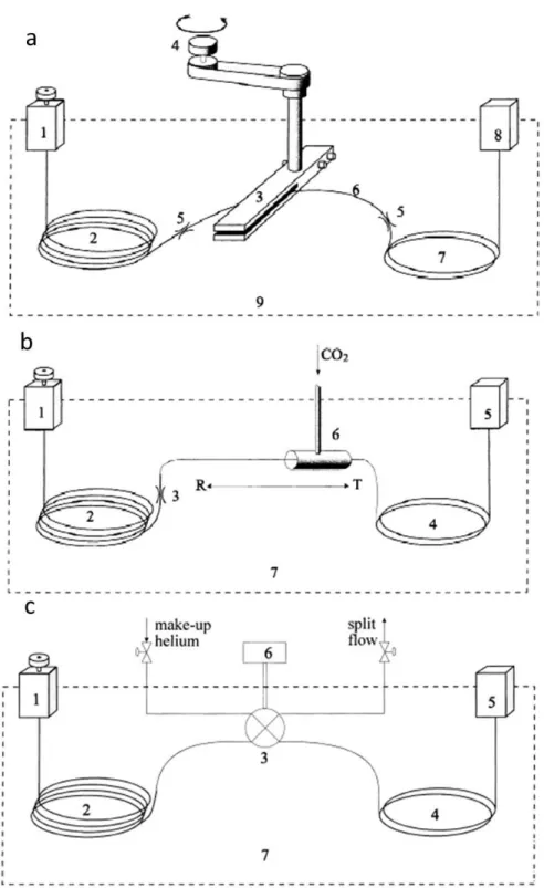
5.11 GC-GC×GC-2FID schematic: a, details the volatile heart-cut stage, b, details the standard GC×GC-FID operation . . . 192 5.12 Schematic of the liquid CO2 re-focussing T-piece . . . 193 5.13 Duplicate injections of a toluene sample with cryo re-focussing off and on
to investigate the effects of re-focussing on separation using GC×GC . . . . 194
5.14 Chromatogram from the GC-GC×GC-2FID instrument run with an NPL
30 ozone precursor component standard . . . 195
5.15 GC-GC×GC-FID chromatogram, demonstrating the grouping of compounds 196
5.16 Breakthrough test results for n-Pentane, Isoprene, Benzene and n-Propane . 198
5.17 Time series ofn-Pentane (upper) and Isoprene (lower) from the GC-GC×GC
(black) and DC-GC (red) instruments . . . 200
5.18 Correlation between the two GC instruments for n-Pentane (upper) and
Isoprene (lower), a linear regression line has been fitted to the data with the equation of the line and R2 for each correlation shown . . . 201
5.19 Typical GC-GC×GC chromatogram from Bachok from 01/02/2014 at 22:32 202
5.20 Different meteorological periods experienced at Bachok, Malaysia . . . 203
5.21 GC-GC×GC chromatogram from Bachok that is representative of a clean
marine influenced air mass from 19/01/2014 at 07:24 . . . 204
5.22 GC-GC×GC chromatogram from Bachok that is representative of a highly
polluted air mass from 20/01/2014 at 07:21 . . . 205 5.23 Time series of isoprene (lower) and toluene (upper) during the Bachok
cam-paign. . . 206 5.24 Diurnal profiles of NO, NO2, isoprene, toluene,n-pentane and C10aliphatic
species . . . 207 5.25 Images of local rubbish burning from the surrounding area . . . 208 5.26 Comparison time series (left panel) and correlations (right panel) of toluene
2.1 Contents of the two NPL standards, along with measured mixing ratios and
associated uncertainties . . . 69
2.2 Individually identified VOC mixing ratios, grouped by functionality, ordered by carbon number . . . 77
2.3 Grouped VOC mixing ratio and the number of isomers in each group . . . . 81
2.4 Comparison of London, North Kensington, LA and Bakersfield . . . 84
2.5 Room Temperature Rate Constants for the Gas-Phase Reactions of OH Radicals with C12 Aliphatic Compounds82,179–182. . . 89
2.6 Primary hydrocarbon OH reactivity (s-1) divided by emission source for winter and summer . . . 92
2.7 Fuel use changes for the UK178 . . . 98
3.1 Max, mean and minimum observed ratios during the winter and summer campaign for b:t and b:135tmb. . . 114
3.2 VOC species included in the MCM modelling of OH reactivity during the ClearfLo summer campaign with their associated OH rate constants.82 . . . 129
3.3 Grouped VOC species included in the MCM modelling of OH reactivity with their associated OH rate constants82 . . . 130
4.1 NK and MR mixing ratios in pptv measured using a PTR-MS245 . . . 146
4.2 Correlation of all individually quantified VOCs with ethanol . . . 169
4.3 Correlation of the grouped species with ethanol . . . 170
5.1 Gradient, intercepts and R2 values for breakthrough test compounds . . . . 199
A.1 Winter correlations of saturated aliphatic species . . . 217
A.2 Winter correlations of saturated and unsaturated aliphatic species . . . 218
A.4 Winter correlations of saturated aliphatic and the grouped species . . . 220
A.5 Winter correlations of unsaturated aliphatic species . . . 220
A.6 Winter correlations of unsaturated aliphatic and aromatic species . . . 221
A.7 Winter correlations of unsaturated aliphatic and grouped species . . . 222
A.8 Winter correlations of the aromatic species . . . 222
A.9 Winter correlations of the aromatic and grouped species . . . 223
A.10 Winter correlations of the grouped species . . . 223
A.11 Winter correlations of measured species with dichloromethane . . . 224
A.12 Summer correlations of saturated aliphatic species . . . 225
A.13 Summer correlations of saturated and unsaturated aliphatic species . . . 226
A.14 Summer correlations of saturated aliphatic and aromatic species . . . 226
A.15 Summer correlations of saturated aliphatic and grouped species . . . 227
A.16 Summer correlation of unsaturated aliphatic species . . . 227
A.17 Summer correlations of unsaturated aliphatic and aromatic species . . . 228
A.18 Summer correlation of unsaturated aliphatic and grouped species . . . 229
A.19 Summer correlations of aromatic species . . . 229
A.20 Summer correlations of aromatic and grouped species . . . 230
A.21 Summer correlations of grouped species . . . 230
A.22 Summer correlations of the two halogenated species with the other species measured . . . 231
A.23 Winter correlation of OVOC species . . . 232
A.24 Winter correlations of saturated aliphatic compounds with OVOCs . . . 233
A.25 Winter correlations of unsaturated aliphatic compounds with OVOCs . . . 234
A.26 Winter correlations of aromatic compounds with OVOCs . . . 235
A.27 Winter correlations of grouped species with OVOCs . . . 236
A.28 Summer correlation of OVOC species . . . 237
A.29 Summer correlations of saturated aliphatic compounds with OVOCs . . . . 238
A.30 Summer correlations of unsaturated aliphatic compounds with OVOCs . . . 239
A.31 Summer correlations of aromatic compounds with OVOCs . . . 240
A.32 Summer correlations of grouped species with OVOCs . . . 241
Firstly, I would like to thank NERC for funding my PhD.
Secondly, to my supervisors Dr Jacqui Hamilton and Dr James Lee, thank you for putting your faith in me and pushing me through my comfort zone. You are both an inspiration to me and I hope to accomplish even half as much as you have.
A big thank you must go to Dr Richard Lidster and Dr Jimmy Hopkins. Your knowl-edge and time were priceless and much appreciated.
To the whole Atmospheric Chemistry group at York, thanks to everyone for all your help and support. The many amazing nights out and laughs were a major part of why I didn’t lose my mind. Special mention to Kelly....I feel your pain now and you’re right, never again!
Many thanks go to the people of the ClearfLo campaign; Lisa, Dan, Nicky, James, Bill, Dave and many others too numerous to mention. Thank you for all the useful discussions and good times during field work. Thanks to the Bachok IOF people, specifically Iq and Dave for taking care of me when I was ill and making sure the instrument didn’t die. Brian Bandy....what can I say....it was interesting working with you, you’re a great bloke and I especially enjoyed playing pool with you.
Particular thanks go to my family for all your love and support. Mam, Dad, Alex, Grandma Pat, Lee and the Dunmores, you have given me the courage to strive to the highest possible level. To those no longer here, I hope I have made you proud.
Last, and definitely not least, my husband. Chris, you put up with my craziness and believed in me; even when I had given up hope. Your support meant the world, I love you.
The research described in this thesis is original work, which I undertook at the Uni-versity of York during 2011-2015. Except where stated, all of the work contained within this thesis represents the original contribution of the author. Some parts of this thesis have been published in journals; where items were published jointly with collaborators, the author of this thesis is responsible for the material presented here. For each published item the primary author is the first listed author. Publications are listed at the beginning of the chapter to which they relate.
The copyright of this thesis rests with the author. Any quotations from it should be acknowledged appropriately.
The role of volatile organic
1.1
Air quality
The negative impacts of poor air quality have long been studied, from the 1100’s in Egypt,
to 13th Century London,1 and through the London and Los Angeles Smog episodes of the
1950’s2 to the present day. These events have motivated the funding of research into
atmospheric science and from this, policy regulations can be put into place to improve future air quality. Studies of urban areas have increased dramatically over the past two decades, where poor air quality is often associated with the high emissions due to large populations.
Residents in urban areas can be significantly affected by the health problems associated
with poor air quality. Ozone (O3) and particulate matter (PM) are two of the most
important pollutants, with exposure causing an estimated 17,400 and 458,000 premature
deaths in Europe respectively in 2011.3 There has been a small decrease in the observed
trend in the direct emission of PM, however no discernible trend has been observed for O3
in Europe.3 Another pollutant of interest is nitrogen dioxide (NO2) which although it has shown a decreasing trend in the past decade, the increased use of diesel-powered vehicles
has resulted in an increase in direct emissions into the atmosphere.3 New techniques have
allowed for an estimate to be made of the mortality expected from long-term exposure to
NO2, with an approximate 5,879 premature deaths in London for the year 2010.4
Megacities are classified as urban areas with a population of more than 10 million. Figure 1.1 shows the evolution of urban land use and the growth of urban areas into megacities, from only 10 cities in 1990 to 28 in 2014 and a projected 40 by 2030.5 There is also growth in the overall percentage of the World that is classified as urban, as well as an increase in larger cities in general; cities with a population of 5-10 million and 1-5 million
are predicted to increase from 21 in 1990 to 63 in 2030 and 239 to 558 respectively.5
Megacities present many challenges for air quality, not simply as a source of local air pollution but also by contributing to transboundary pollution which can lead to increases in global concentrations.6,7Human activities within these cities emit primary PM as well as
nitrogen oxides (NOx, the sum of nitrogen monoxide (NO) and NO2) and volatile organic
compounds (VOCs) as primary pollutants, which can then react in the atmosphere to create secondary pollutants, such as O3, secondary organic aerosol and secondary inorganic aerosol (SOA and SIA, different types of particulate matter).
Comparing pollution concentrations in different megacities can provide information about possible sources and how effective individual countries are at controlling emissions.
Figure 1.1: Percentage of urban land use and city population for 1990 (top), 2014 (middle) and predicted for 2030 (bottom). Data maps taken from the United Nations, Department for Economic and Social Affairs, http://esa.un.org/unpd/wup/Maps/CityDistribution/CityPopulation/CityPop.aspx
Studies have shown that it is possible to pinpoint emission sources through the statistical
analysis of ambient air pollution concentrations.8 The UN estimates that over 600 million
people in urban areas worldwide are exposed to potentially harmful levels of air pollution, mainly from traffic emissions.9 This is supported by Parrishet al., (2009), who found that emissions from gasoline-fuelled vehicles dominate in megacities, indicating that vehicular emission controls are an important policy to put in place.8 This is particularly important
carbon monoxide (CO) and VOCs. A new area for concern is the rapid growth in the use of diesel-powered vehicles in Europe which could potentially change the composition of emissions in urban areas. The ramifications of this change are discussed in detail in Chapter 2.
1.1.1 Health effects of air pollution
The health effects of both short- and long-term exposure to air pollution have been studied extensively over the past three decades (see the World Health Organisation (WHO), “Re-view of evidence on health aspects of air pollution” report, (REVIHAAP) and references within).10 By definition, an air pollutant is a compound that could have an adverse effect
on either humans, animals, vegetation or materials.11 Exposure could be from inhalation,
ingestion or dermal contact (although this is only a minor route).11
Figure 1.2: Summary of the key health effects associated with exposure to the major pollutants: benzo(a)pyrene (BaP), NO2, O3, PM and sulphur dioxide (SO2).(modif iedf rom12,13 )
Health effects from exposure to air pollution can range in severity and affect different bodily systems and/or organs as shown in Figure 1.2. This figure shows the main health effects associated with specific pollutants. These effects could be anything from minor respiratory symptoms to cardiovascular diseases, culminating in increased morbidity and
premature mortality.11 The EU has implemented exposure guidelines, levels above which
the pollutant would adversely affect human health. However, many EU countries are
reviewed a significant number of recent publications that suggest exposure to pollution at levels significantly lower than the 2005 guidelines can still adversely affect human health.10
The direct emission of VOCs and PM, and the production of O3, SOA and SIA, can
affect health in different ways and to varying degrees. This is dependent on multiple factors; the specific type of pollutant and its concentration, duration of exposure, any other pollutants present and the individuals susceptibility to any particular ailments (i.e. pre-existing medical conditions).11 These effects are particularly relevant for megacities due to the high population densities present there.
Some VOCs are classified as carcinogenic, likely to adversely affect health just from
their direct emission, such as benzene and polycyclic aromatic hydrocarbons (PAHs).3
The WHO have estimated that an exposure to benzene concentrations of only 1.7µg m−3
over a person’s lifetime could cause a cancer risk to up to 10 out of every one million people exposed.14This is quite a small value considering the regulated annual average of benzene for the EU is 5µg m−3.15 Also of note are the interactions between different VOCs. The VOCs themselves may not be harmful, but the combination of two or more in a pollutant
mixture such as the emission of vehicle exhaust, could cause an adverse health effect.14
The health effects associated with exposure to VOCs range from respiratory symptoms
to neurological conditions such as headaches, nausea and depression.14,16,17 However, the
effect of VOCs on health is not limited to direct emission, the secondary pollutants formed
through reactions of VOCs in the atmosphere (i.e.O3 and SOA) can also lead to adverse
health effects.
Ozone is an important, and highly toxic, component of photochemical smog.18
Expo-sure to O3can cause a variety of adverse health effects, such as reductions in lung function and other respiratory conditions.18This is exacerbated in people with pre-existing medical
conditions such as asthma.19The WHO 2005 guideline for a mean 8 hour exposure to O3is
100µg m−3, although it is likely that exposure below this threshold will also cause adverse health effects. Bellet al., (2007) analysed the results of nearly 40 studies and found that a short-term exposure to O3 can cause a statistically increased mortality, particularly from
either cardiovascular or respiratory illnesses.20 Long-term exposure to O3 can also have
effects on health.19 Recent studies have postulated that exposure to levels of O3 from the year 2000, could potentially have caused 0.20 – 0.47 million premature deaths globally for the year.21,22
are not limited to, premature mortality and morbidity, pulmonary disease and respiratory illnesses, specifically asthma. Long-term exposure to PM has been found to dominate
the health burden of the population.19,23 No lower limit has been found at which the
exposure to PM will not cause health impairment and as such it is dangerous when people are exposed to even relatively small amounts.18 The size of particles (discussed in detail in Section 1.2.3) is particularly important to consider when determining to what extent health will be affected. Small particles can reach the gas-exchange region of the lungs and very small particles have been found to be able to pass through to other organs in the
body therefore causing more damage.18,24–26 Additionally, there is increasing evidence of
effects on cardiorespiratory health and the central nervous system through exposure to ultrafine particles.10,19,26
1.1.2 Climate effects of air pollution
Drivers of climate change are anthropogenic species and processes that can alter the Earth’s energy budget. The strengths of these drivers to change the energy flux is quanti-fied as radiative forcing in units of Watts per square metre (W m−2).27 The contribution of the emissions of various species to radiative forcing is shown in the well-know Inter-governmental Panel on Climate Change (IPCC) graph in Figure 1.3. This is the latest version from the fifth IPCC Assessment Report (AR5) which shows the contributions of,
not only emissions, but also the atmospheric drivers which result from those emissions.28
A positive radiative forcing value indicates warming of the Earth’s surface, with neg-ative values showing the opposite (surface cooling). Estimates of radineg-ative forcing are based on either in-situ and/or remote observations, properties of greenhouse gases and aerosols, and calculations from numerical models that are used to represent the observed processes. Figure 1.3 shows that the total anthropogenic radiative forcing for 2011 relative
to 1750 is positive (2.29 W m−2), leading to an uptake of energy by the climate system.
This value is 43% higher than that reported in the previous IPCC report, (AR4, total anthropogenic radiative forcing for the year 2005 relative to 1750, 1.6 W m−2). It is likely this large increase is due to the combination of the continued growth in the concentrations of most greenhouse gases and improved estimates of the radiative forcing from aerosols, which indicated a weaker net cooling effect than previous reports (i.e.a negative radiative forcing).28
Figure 1.3: Radiative forcing estimates for 2011 relative to 1750 and aggregated uncertainties for the main drivers of climate change. Values are global average radiative forcing, partitioned according to emitted compounds or processes that result in a combination of drivers. Best estimates of net radiative forcing are shown with black diamonds with corresponding uncertainty intervals; the numerical values are provided on the right of the figure, together with the confidence level in the net forcing (VH - very high, H - high, M - medium, L - low and VL - very low). Albedo forcing due to black carbon on snow and ice is included in the black carbon aerosol bar. Small forcings due to contrails (0.05 W m−2, including contrail induced cirrus), and HFCs, PFCs, and SF
6 (total 0.03 W m−2)
are not shown. Concentration-based radiative forcings for gases can be obtained by summing the like-coloured bars. Volcanic forcing is not included as its episodic nature makes it difficult to compare to other forcing mechanisms. Total anthropogenic radiative forcing is provided for three different years relative to 1750.28
decades. O3 is a radiatively active greenhouse gas with current radiative forcing estimates for 2011 of +0.35 W m−2 for total O3.19 The majority of the radiative forcing from O3
can be attributed to increases in the emission of O3 precursor species, such as NOx,
CO, non-methane VOCS (NMVOCs) and methane (CH4). Methane, while an important
precursor of O3, is also a strong greenhouse gas in its own right (it has a higher radiative forcing value than O3, seen in Figure 1.3) and will be discussed in more detail later. The remaining O3 precursor species have a variety of indirect effects on climate which are not
can be oxidised to carbon dioxide (CO2) which has an additional warming effect although this is relatively small, in the order of +0.02 to +0.09 W m−2.28,29
Methane is one of the most important greenhouse gases, it has a radiative forcing value
of +0.5 ±0.05 W m−2 which makes up approximately 28% of the total radiative forcing
from non-CO2constituents in 2010.30It is a powerful infra-red absorber, making it a more
efficient greenhouse gas than CO2 (28 times more efficient over a century time-scale).31
The atmospheric lifetime of methane is approximately 10 years,31–33so its potential effects on climate are substantial.
Both anthropogenic and biogenic source NMVOCs can contribute to climate warming,
although through different pathways. Anthropogenic NMVOCs affect both O3 production
and increases in the lifetime of methane. A number of studies have shown the correlation between increased NMVOC and CO concentrations and the increased radiative forcings
from O3 and methane.29,34–38 Biogenic VOCs (BVOCs) are particularly important in
re-mote forested regions where there are typically low NOx but high VOC concentrations.
Oxidation of these BVOCs produces peroxy radicals, but the lack of sufficient NOx leads
to inhibited O3 formation.39 BVOCs can then further decrease the O3 concentrations
though direct VOC + O3 reactions. This, combined with the removal of oxidant species
during VOC oxidation, reduces the oxidising capacity of the atmosphere.40 This increases
the lifetime of methane, as its main sink (the OH radical) is removed from the
atmo-sphere through reactions with the BVOCs,41,42 thus increasing the warming that occurs.
Additionally, BVOCs can contribute to aerosol formation as some of their oxidation
prod-ucts can undergo gas-to-particle partitioning to form SOA.43 This both directly affects
the Earth’s radiation budget through the scattering of solar radiation by aerosols and
indirectly from the formation of cloud condensation nuclei (CCN).44,45
The relationship between climate and aerosols is less understood and more complex,
as they have both warming and cooling effects.18 Aerosols can affect climate directly
through aerosol-radiation effects and indirectly via aerosol-cloud effects.19 The former
is from aerosol particles either absorbing or scattering radiation which can warm the atmosphere and cool the Earth’s surface respectively. The latter is based on the capability of particles to act as CCN. These are usually particles with diameters larger than 50-100 nm that are activated in rising air masses to form cloud droplets. If there is a sufficient concentration of cloud droplets, there is a higher cloud albedo, causing back scattering of solar radiation, reduced precipitation, and a longer lifetime of the clouds. This is a cooling
climate driver where the Earth’s surface is shaded from solar radiation.46 It is estimated that the cooling exceeds the warming effects from aerosols. However there is quite a high level of uncertainty, indicated by the large error bars in Figure 1.3, about the overall effect of aerosols on climate.28
1.1.3 Air quality and climate change
Air quality and climate change are usually considered as separate issues for many areas of science and policy. However, they are highly connected and linked through (1) emissions to the atmosphere, (2) atmospheric properties, processes and chemistry, and (3) mitigation
strategies.19There are many common sources that emit both climate change driving forcers
and air quality pollutants. Once these pollutants have been emitted into the atmosphere, they have a variety of atmospheric properties, which can influence whether they have
a direct or indirect effect on radiative forcing. Their lifetime in the atmosphere and
the atmospheric chemical processes they are involved in can also influence their effect on human health and the ecosystem. Current mitigation strategies can potentially both
improve air quality and mitigate climate change, termed win-win. However, some so
called win-lose or trade-off strategies only provide benefits to one area and exacerbate the
situation in another.19 This is shown in Figure 1.4, where for example, the increased use
of diesel cars to reduce CO2 emissions (a climate change benefit) resulted in an increased
emission of NOx and PM (a detriment to air quality).
There is still a significant amount of work to be done to fill knowledge gaps, despite the recognition that there are strong links between climate change and air pollution. This needs to be in both scientific and political communities through the coordination of future mitigation and/or adaptation strategies. These strategies must be put into the broader context of the big picture, that the atmosphere is a limited resource. Thus future policies can be implemented with fewer unforeseen, potentially negative, consequences arising. However, there are challenges to this process. Specifically what feedback effects do climate policies have on air quality and vice versa.
Figure 1.4: Trade-offs from policies and technologies to tackle climate change and air quality19,47–49
1.2
Volatile organic compounds
The focus of this thesis will be on one specific type of pollutant, VOCs, and the effects
they have on PM and O3 concentrations. It is important to measure VOCs as they play
a key role in the atmosphere through reactions that determine concentrations of other
important atmospheric species, such as PM and O3.50 VOC is a term used to describe a
very large group of vapour-phase organic compounds, excluding CO and CO2but including
hydrocarbons, oxygenated, halogenated and other hetero atomic compounds,39which play
a central role in atmospheric chemistry; and have both natural and anthropogenic sources. VOCs can be primary and/or secondary pollutants, and react in the atmosphere at rates
which can vary by orders of magnitudes.51
As a large group of compounds with differing volatilities, VOCs can be broadly grouped based on their effective saturation concentrations (C*, inµg m−3), an empirical expression of volatility. This can be calculated using Equation 1.1 where; Cvapi (µg m−3) is the concentration of the speciesiin the vapor phase, COA(µg m−3) is the total organic aerosol
R is the gas constant, T (K) is the temperature, Mi (g mol−1) is the molecular weight of
the speciesi,ζ0i is the molarity-based activity coefficent (assumed to be 1) and PoL,i (Torr) is the saturation vapor pressure of pure speciesiat temperature T.52,53 As the saturation concentrations decrease, the volatility also drops and the individual VOC species is more likely to partition from the gas phase into the particulate phase as shown in the lower
panel of Figure 1.5 for the reaction of O3 withα-pinene, where the white and green bars
represent species in the gas and particle phases respectively.53
Ci∗ = C vap i .COA Ciaer = Mi.106.ζ 0 i.PL,io 760.R.T (1.1)
Figure 1.5: Gas-to-particle partitioning diagram of products from the reaction of O3 andα-pinene. One dimen-sional volatility basis set product distribution, for each log10C* bin. Partitioning is shown for approximately 10
µg m−3 of SOA, obtained from the oxidation of 100µg m−3 ofα-pinene, with condensed-phase OA in green and
vapor-phase products in white.(modif iedf rom53)
VOC - Volatile organic compounds (C∗ of > 106 µg m−3, white shaded region in
Fig-ure 1.5). These compounds exist in the gas phase under ambient conditions.
shaded region in Figure 1.5), exist almost entirely in the gas phase under ambient condi-tions, only a small portion of the organic mass is highlighted as being in the particle phase in Figure 1.5.53,54
SVOC - Semi-volatile organic compounds (C∗of 1 to 103µg m−3, light green shaded region in Figure 1.5), can exist in both the gas and particle phases at ambient conditions.53,54
LVOC - Low volatility organic compounds (C∗ of 10−2 to 1 µg m−3, light red shaded
region in Figure 1.5), exist predominantly in the particle phase with some small gas-phase fractions.53,54
ELVOC - Extremely low volatility organic compounds (C∗ of<10−3 µg m−3, gray shaded region in Figure 1.5), resides almost entirely in the particle phase at ambient condi-tions.53,54
1.2.1 Emission sources of volatile organic compounds
VOCs are released into the atmosphere from both natural emission from the Earth’s veg-etation (termed biogenic emission) and as a result of human activities (anthropogenic emission). By definition, anthropogenic VOCs are either directly emitted to the
atmo-sphere or produced during combustion.55 The dominant sources of these VOCs in urban
areas is from the use of fossil fuels in the transport sector and industrial processes.55 Bio-genic VOCs (BVOCs) are species that are directly emitted to the atmosphere from the Earth’s surface. These can generally be categorised into emissions from terrestrial
veg-etation, soils and the ocean.56,57 However, the line between anthropogenic and biogenic
sources of VOCs is not straightforward. Many VOCs can be produced or emitted from both sources. Although the emission from anthropogenic sources is particularly important in urban areas and megacities, biogenic emissions of VOCs worldwide are approximately
ten times larger, by mass, than anthropogenic emissions.58–60
Concentrations of VOCs do not continue to increase with time so there must be one or more removal processes or sinks. The most important of these sinks is through gas phase chemical oxidation primarily with the hydroxyl (
·
OH) radical, but also with O3 andnitrate (NO3
·
) and halogen radicals.61,62 Some of the gas phase VOCs can also absorbsunlight and be photolysed. These oxidised compounds can then be removed by dry or wet deposition to the Earth’s surface through absorption to vegetation58,63 or in rain,64,65 respectively and either through adsorption onto the surface, absorption into aerosols or
partitioning into aerosols.66 This will be discussed in more detail in Section 1.2.2.
1.2.1.1 Anthropogenic sources
There are many different and varied anthropogenic sources of VOCs. The three main global sources of anthropogenic VOCs are use of fossil fuels, industrial processes and biofuel combustion. VOC emissions from the use of fossil fuel in vehicles is the most
important global anthropogenic source of VOCs.55Emissions from industrial applications
such as manufacturing, residential heating and cooking are small in comparison to fossil fuel use but can be important in some regions. For example, in China where approximately 30% of total Chinese anthropogenic VOC emissions, for the year 2000, were from the
substantial use of coal and biofuels in residential cooking.67 Fugitive emission of VOCs
through evaporation can also occur during the distribution and storage of fuel, typically from ships, road tankers and fuel stations. Evaporative emissions from fuel stations are
particularly important on local and regional scales, not just from concerns about O3
formation but also adverse health effects. There can be substantial emissions of toxic and carcinogenic species, such as benzene.55
Industrial process emissions are largely from solvent use in paints, adhesives and inks etc., where the solvent evaporates after use. This can lead to much higher emissions during
warm seasons.68Other important industrial uses are the manufacture of pharmaceuticals,
metal surface cleaning, extraction of oil seeds and printing. However, many industries have had to reduce emissions due to policy interventions. This has lead to companies
either recycling the VOCs emitted or thermally destroying them.55
The primary energy source in developing countries is the combustion of biomass. The emissions are overwhelming from the residential sector through heating and cooking. More recently, there has been a large influx of emissions from the combustion of biofuels in the transport sector. Largely from, mainly Brazil but also other countries, the use of pure ethanol and blended ethanol and gasoline as vehicle fuels.55This will be discussed in more detail in Chapter 4, Section 4.2.
1.2.1.2 Biogenic sources
BVOCs are predominantly emitted from the foliage of terrestrial vegetation. This en-compasses both natural vegetation (trees, shrubs, grasses, ferns and mosses) and
minor sources from ocean and soil emissions that can contribute to the global
concen-trations of BVOCs.57 Although many thousands of species can be emitted,68,69 those
emitted in the largest concentrations are isoprene, monoterpenes, sesquiterpenes and a selection of oxygenated VOCs (OVOCs), specifically methanol, acetone, ethanol and ac-etaldehyde.19,56,57,70
1.2.2 Chemistry of volatile organic compounds
The degradation reactions of VOCs have been well documented. These reactions are
particularly important due to the generation of numerous secondary pollutants, specifically
O3 and SOA. VOCs emitted into the troposphere, react with radical species (such as the
·
OH and hydroperoxyl (HO2
·
) radicals) and sunlight then, in the presence of NOx, formO3, a simplified reaction scheme is shown in Figure 1.6. A key part of this scheme is the catalytic cycling of radicals which allow for a sustained concentration of the
·
OH radical during the day. This helps the propagation of further reactions.39Figure 1.6: Simplified reaction cycle through which VOCs form O371
The chemistry of VOCs is extremely complex as there are many hundreds of emitted species that possess a variety of physico-chemical properties due to differences in their
structure and functional group.72 The degradation mechanism of each individual VOC
is essentially unique.72 A further complication to understanding VOC chemistry, is that
intermediate organic products to be generated. These possess a wide variety of properties
which influence their potential to form O3 and SOA. The intermediate species can also
undergo secondary reactions to produce O3 thus further increasing the complexity. It is
vital to have intensive measurement studies on VOC emissions, so that the intermediate
oxidised species produced during atmospheric reactions, such as the alkyl peroxy (RO
·
2)and alkoxy (RO
·
) radicals (shown in Figure 1.6), can be modelled as they cannot usuallybe measured due to their very short lifetimes in the atmosphere. These intermediate species are the route to form increased amounts of O3.
1.2.2.1 Reaction of volatile organic compounds with radicals
The most important daytime radical is the
·
OH radical, as it is usually the first and ratedetermining step in the removal of many trace species (Figure 1.7).73 The
·
OH radicalreacts with a large number of pollutants, forming oxidised species that can be more easily
removed from the atmosphere, leading to it been termed the “atmospheric detergent”.73–75
Figure 1.7: A simple schematic diagram through which the reactions of OH and HO2radicals are shown to produce secondary pollutants such as O3, PM and SOA.76Numbers in red correspond to equations included in the body of
text.
The main source of the
·
OH radical is through the photolysis of O3 to formelectroni-cally excited O(1D), (Equation 1.2), which then reacts with water vapour (H
2O) to form two
·
OH radicals, (Equation 1.3). Only 10% of the O(1D) actually forms the·
OH radical;while the other 90% relaxes to form O(3P) which reforms O
O3+hv−−→O(1D) + O2 (λ ≤ 320 nm) (1.2)
O(1D) + H2O−−→2
·
OH (1.3)O(1D) + M−−→O(3P) + M where M−−N2or O2 (1.4)
O(3P) + O2+ M−−→O3+ M where M−−air molecules (1.5)
However, in urban areas that are heavily polluted, there are other mechanisms that
become available for the formation of the
·
OH radical. This is mainly through thepho-tolysis of nitrous acid (HONO, Equation 1.6). In areas with high concentrations of NO, reactions with HO2
·
radicals can also generate significant concentrations of·
OH radicals, Equation 1.7.HONO +hv−−−−−−→λ<400nm
·
OH + NO (1.6)HO2
·
+ NO−−→·
OH + NO2 (1.7)During the daytime,
·
OH radicals can initiate the degradation of many atmospherictrace gases, particularly VOCs,78,79with the
·
OH radical budget in the atmosphere beingcontrolled by the concentrations of O3, water, sunlight, VOCs, CO and NOx.79 As the
·
OH radical source is mainly photochemical, during the night, the NO3
·
radical (formedthrough the reaction of NO2 and O3 in Equation 1.8) takes over as the most important
reactive oxidant in the troposphere; even though it is less reactive.80 The NO3
·
radical isnot as important as the
·
OH radical during the day, due to it being rapidly photolysed toNO2 and O3 in the presence of solar radiation (Equations 1.9 and 1.5).73,80 The reaction
of VOCs with O3 is also important both day and night, particularly with unsaturated
compounds through addition across the double bond.81
NO2+ O3 −−→NO3
·
+ O2 (1.8)The reactions of VOCs with the
·
OH radical is the key removal mechanism for the majority of VOCs in urban atmospheres. This cycle is also responsible for the production of tropospheric O3, in the presence of NOx. Generally, the reaction of·
OH radicals withorganic species such as VOCs isviahydrogen atom abstraction to form water and an alkyl
radical (R
·
), shown in Equation 1.10. The alkyl radical can then react with molecularoxygen (O2) to form alkyl peroxy radicals (RO2
·
, Equation 1.11), the subsequent reactionof these with NO forms an alkoxy radical (RO
·
) and NO2, Equation 1.12.RH +
·
OH−−→R·
+ H2O (1.10)R
·
+ O2−−→M RO2·
(1.11)NO + RO2
·
−−→RO·
+ NO2 (1.12)NO + RO2
·
−−→RONO2+ M (1.13)The NO2 produced in Equation 1.12 photo-dissociates to form O(3P) in Equation 1.14
which can form a molecule of O3 via Equation 1.5.
NO2+ hv−−→NO + O(3P) (1.14)
The RO2
·
radical resulting from Equation 1.11 can also react with HO2·
, other RO2·
radicals and NO2 to form a series of products, detailed below in Equations 1.15-1.20. The
products from Equation 1.20 are peroxyacyl nitrates (PAN).82
RO2
·
+ HO2·
−−→ROOH (1.15)RO2
·
+ HO2·
−−→R−−O + H2O + O2 (1.16)RO2
·
+ HO2·
−−→ROH + O3 (1.18)RO2
·
+ R0O2·
−−→products (1.19)RO2
·
+ NO2 −−)−−*RO2NO2(PAN) (1.20)The RO
·
radical, formed through Equation 1.12 can react with a number of differentspecies, depending on the structure of the R hydrocarbon chain. The reaction of RO
·
radicals with O2 is one of the most important (Equation 1.21), particularly if the R chain
is an alkane. From this reaction a carbonyl compound (R=O) and a HO2
·
radical isformed. The HO2
·
radical can then react via Equation 1.7 to re-form an·
OH radical.The NO2 from this reaction will dissociate and eventually form O3 (Equations 1.14 and
1.5). This completes a catalytic cycle, as the
·
OH radical is regenerated, as seen previouslyin Figure 1.6. An oxidised product and two molecules of O3 are also formed.
RO
·
+ O2 −−→R0CHO + HO2·
(1.21)As discussed previously, the lifetime of many species in the atmosphere are governed
by the concentration of the
·
OH radical. The lifetime of VOCs is slightly more complex,usually the reaction with the
·
OH radical dominates however this is dependent on theindividual VOC. The reactions with O3 and/or the NO3
·
radical can dominate due tohigher concentrations of them in comparison to the
·
OH radical. Lifetimes of VOCs canvary from several months for some alkanes to just a few hours or less for alkenes and even minutes or seconds for very reactive species such as sesquiterpenes. The lifetime of
VOCs with respect to the
·
OH radical can be calculated by Equation 1.22; where τ isthe lifetime, which is the time it takes for the concentration of compound i to fall to 1e of its initial concentration, kV OCi is the rate constant of compound i and [
·
OH] is the concentration of the hydroxyl radical.τ−− 1
kV OCi·[
·OH
]When conducting studies of VOCs and their reaction with the
·
OH radical, anotherimportant consideration is
·
OH reactivity, k’. This is the product of multiplying thebimolecular rate coefficient for the species Xwhen reacting with the
·
OH radical with its associated concentration.83This is shown in Equation 1.23, where [X] is the concentration andkX,OH is the bimolecular rate coefficient for the speciesXwhen reacting with the·
OHradical. Total
·
OH reactivity (kOH), the inverse of the lifetime of the·
OH radical, canbe calculated by summing the reactivity of all the chemical species under study, shown
in Equation 1.24 and discussed in more detail in Chapter 3.78,83 All these factors are
important when studying the chemistry of urban areas as studies have shown that VOC
concentrations can be the limiting factor for O3 production, (discussed in detail in the
next section).84 kX =kX,OH·[X] (1.23) kOH = n X i=1 kX,OH·[X]i (1.24) 1.2.3 Formation of ozone
O3 can pose a significant threat to health, ecosystems, climate and materials on local,
regional and global scales.3 As such, it is important to fully understand why, despite con-trols in place to decrease concentrations of precursor air pollutants, this has not happened to the degree expected.85
There is no direct emission source of O3 in the atmosphere, rather it is formed through
a chain of photochemical reactions of the precursor gases NOx, VOCs and CO, discussed
previously. The reductions of these precursor gases does not appear to have resulted in
the expected decrease in ambient O3 concentrations in Europe.3 For example, 2012 EU
emissions relative to 2003 were decreased by 30%, 32%, 28% and 15% for NOx, CO,
NMVOCs and CH4 respectively, while O3 did not show any clear trend.3 O3 formation is
extremely complex, further compounded by the huge number of VOCs involved. This can have an impact on how regulations for emission reductions are constructed as there are numerous sources of VOCs and their oxidation pathways are complex.
The meteorology of the area where measurements are taken should also being taken
is the correlation between O3 formation and atmospheric temperature.86,87 It has been
shown that the relationship between the daily O3 concentration and temperature is non
linear, where O3 concentration appears to show no dependence on temperatures below
20-25◦C, but is strongly dependent on temperatures above 30◦C.88–92 Historically, the
major O3pollution episodes have been shown to correlate with slow-moving, high-pressure
weather systems combined with high concentrations of VOCs. This effect is increased when these meteorological conditions occur during summer, as this is the time with the
greatest amount of sunlight thus photochemical reactions are at a maximum.93,94 Another
important factor associated with the meteorology is that the conditions can determine
whether O3 precursor species, such as VOCs and NOx, are either contained in the local
region or transported to other regions thus likely affecting the air quality in surrounding areas.
Haagen-Smit and Fox (1954) first plotted a graph (Figure 1.8) which shows how con-centrations of O3 relate to mixtures of VOCs and NOx in the region under investigation.2 This is called an isopleth graph, showing the effect of reducing VOC and NOx levels on O3 concentrations and is an empirical representation of the VOC-NOx-O3 relationship.51The location of a particular point on the O3 isopleth graph is defined as the ratio of VOC and
NOx at that point. This is important to consider in the VOC-NOx-O3 relationship and
shows the major effects of reducing VOC and/or NOx concentrations on corresponding
O3 concentrations.2
Kleinman (1994) proposed an addition to the original isopleth graphs by schematically
showing how the O3 production rate can be limited by either VOCs or NOx through
the use of a Empirical Kinetic Modelling Approach (EKMA) diagram, shown in
Fig-ure 1.9.95,96 This shows two species limited, opposing regimes and a transitional region
(the diagonal ridge from the lower left to upper right corner in Figure 1.9), where O3 is
equally sensitive to VOCs and NOx; but is relatively insensitive compared to the limited
regimes. The transitional ridge corresponds to a VOC/NOx ratio of approximately 8:1.
This ratio is dependent on individual region factors such as the oxidative chemistry of
that area, initial concentrations of pollutants and available oxidants etc. There are two
very useful regions to consider on this graph which show the chemistry of either relatively unpolluted rural/suburban or polluted urban regions. The right of the transitional ridge
is characteristic of a rural/suburban region which is usually NOx limited. This is shown
con-Figure 1.8: Photochemical ozone formation as a function of the concentrations of VOCs and NOx from vehicle exhaust emissions under different driving conditions.2
centrations, resulting in a high VOC/NOx ratio and is relatively insensitive to changes in VOC concentrations. The left of the transitional ridge is systematic of a polluted area that is VOC limited. This shows the opposite scenario, where reducing VOC concentrations
results in lower peak ambient O3 concentration and thus has a low VOC/NOx ratio.
The VOC-NOx-O3 relationship should be taken into account when implementing
poli-cies specifically for O3 reduction. Depending on the region under scrutiny, the specific
VOC/NOx ratios of that area can be used to customise emission controls.51 However it
is not this simple. The effects of other emission reductions need to be considered with respect to the effects they would have on secondary pollutants. These in themselves can be harmful and have multiple further reactions in the atmosphere. An added complex-ity is the role of biogenic emissions. Depending on the area of study, reductions in the
anthropogenic emissions of VOCs may not produce a correlated reduction in O3
concen-trations if there are significant biogenic sources. This shows how regulations need to take into account all the effects of reducing certain pollutants and a reliable evaluation of the
Figure 1.9: Typical EKMA diagram showing isopleths of 1-hr maximum ozone concentrations (in parts per million by volume (ppm)) calculated as a function of initial VOC and NOx concentrations and the regions of the diagram that are characterized by VOC limitation or NOx limitation. “OH production” refers to the rate of OH photochemical production and “NOx source” refers to the rate at which NOx is emitted into the boundary layer.95,96
1.2.4 Particulate matter in urban areas
Aerosols are defined as the suspension of fine liquid or solid particles in a gas. Aerosols
have a variety of sizes and chemical composition. PM has both natural, (i.e.dust, pollen
and sea-spray) and anthropogenic sources, (such as transportation and industry) and two main sinks, wet and dry deposition. Traffic-related emissions are estimated to contribute
to over 50% of total PM concentrations in urban areas.9 Particles have a number of
prop-erties that should be taken into account when trying to understand the roles they play in atmospheric processes, these are number, concentration, size, mass, chemical composition, and aerodynamic and optical properties.
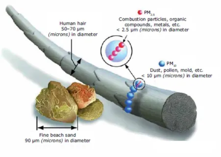
There are two main size ranges measured for air quality; PM10, coarse particles which
encapsulates particles with diameters of 10 µm or less, and PM2.5, fine particles whose
diameters are equal to or less than 2.5µm (shown in Figure 1.10). The sources of coarse
particles are usually mechanical processes, such as grinding, wind and wear. For fine particles, the main source is the gas-to-particle partitioning of low-volatility vapours, with urban areas dominated by combustion emissions.
Figure 1.10: Illustration of the size of PM10and PM2.5 particles in comparison to a human hair and a grain of sand.97,98
Organic aerosols (OA) are particularly important, as they can account for between
20-90% of submicron particulate mass and can be either primary or secondary.99Primary
organic aerosol (POA) is directly emitted into the atmosphere from sources such as biomass burning and fossil fuel consumption. SOA is produced through the oxidation of precursor VOCs to form lower volatility species that have the ability to partition into the aerosol phase (discussed previously in Section 1.2). There has been a slow decline in the direct emission of PM from 2006 to 2012, however emissions in rural and urban backgrounds remained consistent. Even with this decline, exposure limits were exceeded in over 50%
of EU countries in 2012.3 The evolution of both POA and SOA are not fully understood
and as such future research must be carried out on PM, with special emphasis on OA, to determine the sources of PM.
1.3
Measurements of volatile organic compounds
When analysing atmospheric VOCs, there are many techniques to choose from. The
method of choice is dependent on many factors, including the choice of measurement sites
and whether the analysis will be done in-situ i.e. in the field or off-line where samples
are brought back and analysed in the lab. When making observations in the field there are certain criteria which must be met; portability, power consumption, gases required, consumables and the fact that the environment in the field is not always suitable for
sensitive instrumentation, such as mass spectrometers.
1.3.1 Gas chromatography
One of the most common methods of in situ analysis is thermal desorption-gas chro-matography coupled to either a flame ionisation detector or a mass spectrometer
(TD-GC-FID/MS).100 Thermal desorption is a versatile, sample introduction technique which
is used to extract analytes of interest from complex samples such as air. The GC column and oven temperature programme are selected to provide the required selectivity and res-olution of compound peaks. The FID is a detector that gives a response proportional to the number of carbon atoms in the individual species.101 It is widely used due to its fast acquisition rate, broad sensitivities and the fact that it doesn’t produce a signal for
inor-ganic compounds such as CO and CO2.102Compoun