Theses Spring 2020
Representations and representation learning for image aesthetics
Representations and representation learning for image aesthetics
prediction and image enhancement
prediction and image enhancement
Michal Kucer [email protected]
Follow this and additional works at: https://scholarworks.rit.edu/theses
Recommended Citation Recommended Citation
Kucer, Michal, "Representations and representation learning for image aesthetics prediction and image enhancement" (2020). Thesis. Rochester Institute of Technology. Accessed from
This Dissertation is brought to you for free and open access by RIT Scholar Works. It has been accepted for inclusion in Theses by an authorized administrator of RIT Scholar Works. For more information, please contact
by
Michal Kucer
A dissertation submitted in partial fulfillment of the requirements for the degree of Doctor of Philosophy in the Chester F. Carlson Center for Imaging Science
College of Science
Rochester Institute of Technology Spring 2020
Signature of the Author
Accepted by
ROCHESTER, NEW YORK CERTIFICATE OF APPROVAL
Ph.D. DEGREE DISSERTATION
The Ph.D. Degree Dissertation of Michal Kucer has been examined and approved by the dissertation committee as satisfactory for the
dissertation required for the Ph.D. degree in Imaging Science
Dr. David Messinger, Dissertation Advisor
Dr. David Ross, External Chair
Dr. Christopher Kanan
Dr. Alexander C. Loui
Date
Michal Kucer Submitted to the
Chester F. Carlson Center for Imaging Science in partial fulfillment of the requirements
for the Doctor of Philosophy Degree at the Rochester Institute of Technology
Abstract
With the continual improvement in cell phone cameras and improvements in the connectivity of mobile devices, we have seen an exponential increase in the images that are captured, stored and shared on social media. For example, as of July1st2017 Instagram had over 715 million registered users which had posted just shy of 35 billion images. This represented approximately seven and nine-fold increase in the number of users and photos present on Instagram since 2012. Whether the images are stored on personal computers or reside on social networks (e.g. Instagram, Flickr), the sheer number of images calls for methods to determine various image properties, such as object presence or appeal, for the purpose of automatic image management and curation. One of the central problems in consumer photography centers around determining the aesthetic appeal of an image and motivates us to explore questions related to understanding aesthetic preferences, image enhancement and the possibility of using such models on devices with constrained resources.
In this dissertation, we present our work on exploring representations and representation learn-ing approaches for aesthetic inference, composition ranklearn-ing and its application to image enhance-ment. Firstly, we discuss early representations that mainly consisted of expert features, and their possibility to enhance Convolutional Neural Networks (CNN). Secondly, we discuss the ability of resource-constrained CNNs, and the different architecture choices (inputs size and layer depth) in solving various aesthetic inference tasks: binary classification, regression, and image cropping. We show that if trained for solving fine-grained aesthetics inference, such models can rival the cropping performance of other aesthetics-based croppers, however they fall short in comparison to models trained for composition ranking. Lastly, we discuss our work on exploring and identify-ing the design choices in trainidentify-ing composition rankidentify-ing functions, with the goal of usidentify-ing them for image composition enhancement.
did a fantastic job finding balance between encouraging the pursuit of my interests and guiding me towards the completion of my PhD. I could not have imagined having a better advisor and mentor for my doctorate.
Tremendous thank you goes to my thesis committee: Dr. Chrisopher Kanan, Dr. Alexander Loui, Dr. David Ross for their insightful comments and discussions.
I am thankful to my friends: Baabak, Sagar, Will, Martin, Michal, Tereza, Kristan, Clay, and Laura, who’ve been there with me through thick and thin.
During my PhD, I was fortunate to conduct two incredible internships at the Los Alamos National Laboratory (LANL), and Naver Labs Europe. I would like to thank my mentors from LANL, Amanda Ziemann and James Theiler, and Naver, Naila Murray. Furthermore I would like to thank all of the incredible friends that I have made and still keep in touch with.
I have to thank the many friends and people at the Center for Imaging Science. First a big thank you to the fellow PhD students and office mates - Aneesh, Lauren, Mandy, Lucy, Sanghui, Jacob, Ryan just to name a few. Big thanks also goes to Marci, Susan, Beth, Joyce, and all of the staff in CIS.
Thank you to my family in the US - Sandy, Steve, Jeanne, Santosh, Jivan, Nisha, Shaun, Angad - and my host families from Indiana - the Sheeks and the Buchanans.
I would like to thank my parents Peter and Zuzana, who from young age served as my role models and stressed the importance of education. I want to thank my sister Zuzka for her constant encouragement. Without their support, I would not be where I am today.
Table of Contents 5
List of Figures 8
List of Tables 11
1 Introduction 13
1.1 Overview . . . 13
1.2 Contribution and outline . . . 14
2 Background 15 2.1 Standard Approach . . . 15 2.2 Aesthetics Inference . . . 16 2.2.1 Datasets . . . 16 2.2.2 Handcrafted-Features . . . 20 2.2.3 Local Features . . . 27 2.2.4 High-level Features . . . 28 2.2.5 Related Work . . . 30
2.3 Neural Networks and Deep Learning . . . 33
2.3.1 Backpropagation . . . 33
2.3.2 Neuron function . . . 34
2.3.3 Neural Network . . . 34
2.3.4 Implicit learning of ranking functions . . . 37
2.4 Summary . . . 40
3 Multi-Object Salient Foreground Detection 41 3.1 Introduction . . . 41
3.2 Related Work . . . 42
3.3 Algorithm . . . 42 5
3.3.1 Original algorithm . . . 42
3.3.2 Augmenting the background prior . . . 43
3.3.3 Detecting multiple objects . . . 45
3.4 Results . . . 54
3.4.1 Quantitative results and evaluation . . . 54
3.5 Limitations . . . 54
3.6 Conclusion . . . 55
4 Expert knowledge for image aesthetics 56 4.1 Introduction . . . 56
4.2 Datasets . . . 58
4.3 Aesthetic Assessment with Hand-crafted features . . . 59
4.3.1 Learning framework . . . 60
4.3.2 Methodology . . . 60
4.3.3 Comparing different algorithms . . . 61
4.3.4 Feature Elimination . . . 62
4.3.5 Model and feature analysis by categories . . . 66
4.4 Combining the CNN and HC features . . . 69
4.4.1 Choosing baseline CNN features . . . 69
4.4.2 Improving CNN performance with HC features . . . 70
4.5 Conclusion . . . 77
5 Aesthetic Inference for Smart Mobile Devices 79 5.1 Introduction . . . 79 5.2 Related Work . . . 81 5.3 Methodology . . . 81 5.3.1 MobileNet architecture . . . 82 5.3.2 Multi-task Training . . . 83 5.4 Experimental Setup . . . 84 5.4.1 Evaluation Datasets . . . 84 5.4.2 Training details . . . 84 5.4.3 Performance evaluation . . . 86 5.5 Results . . . 86 5.5.1 Aesthetic Inference . . . 86 5.5.2 Image Cropping . . . 89 5.6 Conclusion . . . 90
6 Learning representations for composition ranking 93 6.1 Introduction . . . 93 6.2 Related work . . . 95 6.3 Method . . . 96 6.3.1 Weight initialization. . . 97 6.3.2 Architecture design . . . 97
6.3.3 Learning composition ranking. . . 98
6.4 Experiments . . . 98
6.4.1 Datasets and Experimental results . . . 98
6.4.2 Ablative studies . . . 100
6.4.3 Comparison to the state-of-the-art . . . 102
6.5 Conclusion . . . 106
7 Conclusion and Future Work 107 7.1 Future Work . . . 108
7.1.1 Modeling individual aesthetic preferences . . . 108
7.1.2 Improving representation learning for composition ranking . . . 108
2.1 A standard pipeline used in image aesthetics problems. . . 16 2.2 Figure showing example images from the AVA dataset that demonstrate the kind
of images are used for learning aesthetic functions. We shows examples of images with (a) low mean score, (b) large mean score, (c) low standard deviation in user ratings, and (d) large standard deviation in user ratings. Part (e) show examples of high and low quality images (left and right respectively) along with their dis-tribution of vote counts (which can be used to compute various statistics such as mean) . . . 17 2.3 Figures showing (a) model of the neuron used in neural networks, (b)
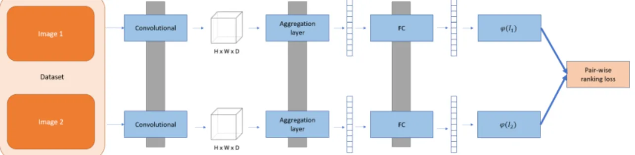
architec-ture of an elementary neural network with a single hidden layer, and (c) the local connectivity of a neuron in a convolutional layer. Source: https://cs231n.github.io/ 33 2.4 A schematic of a Siamese Network used to learn a ranking function via pair-wise
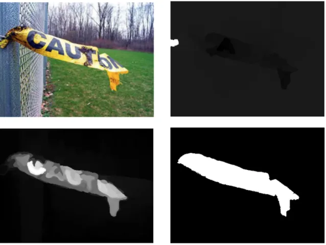
learning. . . 38 3.1 Comparison of the saliency maps after augmenting the background prior: original
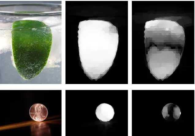
image (top left), Perazzi et al. saliency map (top right), our saliency map (bottom left) and ground truth (bottom right). . . 44 3.2 Images that show the presence of separate objects / object parts in the higher
eigen-vector dimensions. From left: Original image, saliency map constructed from first non-zero eigenvector, saliency map constructed from second non-zero eigenvector, saliency map constructed from third non-zero eigenvector, and the final saliency map, whose construction will be described in later section. . . 46 3.3 Plot of the saliency maps for the first two eigenvectors of the images with a single
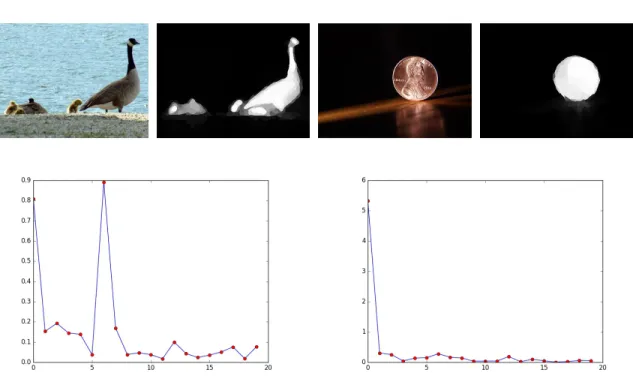
salient object. From left: original image, first zero eigenvector, second non-zero eigenvector. . . 47 3.4 Plots showing the eigenvalue percentage difference plots for sample images with
single / multiple salient objects. . . 48
3.5 Original image (top left) of a scene with one salient object and its corresponding saliency maps as we vary the number of eigenvectors considered for the superpixel embedding: 1 (top right), 2 (bottom left), 3 (bottom right). Map with 1 eigenvec-tors was chosen as the best by our score. . . 50 3.6 Original image (top left) of a scene with multiple salient objects and its
corre-sponding saliency maps as we vary the number of eigenvectors considered for the superpixel embedding: 1 (top right), 2 (bottom left), 3 (bottom right). Map with 3 eigenvectors was chosen as the best by our score. . . 51 3.7 Benchmarks. Performance of the various algorithms on the MSRA [2] dataset. . . 52 3.8 Benchmarks. Performance of the various algorithms on the ImgSal [63] dataset. . 52 3.9 Benchmarks. Performance of the various algorithms on the SED1 [4] dataset. . . 53 4.1 Common photographic rules used in capturing aesthetically pleasing photographs. 57 4.2 Regression performance as the function of topkfeatures on the HB dataset. The
vertical line atk = 75indicated a point after which the regression performance remained approximately constant. . . 64 4.3 Classification performance as the function of the number of top k features HB
dataset. The vertical line atk= 25indicated a point after which the classification performance remained approximately constant . . . 65 4.4 Regression performance as the function of the number of topkfeatures the
differ-ent categories of the HB dataset. The vertical line atk= 40indicated a point after which the regression performance remained approximately constant . . . 67 4.5 Structure of the general pipeline, where we concatenate the HC features with CNN
activations. . . 71 4.6 Regression performance on the HiddenBeauty score for various CNN models and
their combination with HC features. . . 71 4.7 Sample images from the AVA dataset. (a) Top correctly classified images of High
Quality. (b) Top correctly classified images of Low Quality. (c) Incorrectly classi-fied images of High Quality. (d) Incorrectly classiclassi-fied images of Low Quality. (e) Images of High Quality that were correctly classified by concatenating HC fea-tures. (f) Images of Low Quality that were correctly classified by concatenating HC features. . . 74 4.8 Feature Importance (Gain) of thekthfeature. . . 75 4.9 Plot of the distribution of the top performing hand-crafted features across the high
and low quality classes. . . 76 5.1 Examples of photographic images takes by cell-phones. . . 80 5.2 Figure showing the high-level architecture of our model with the multiple outputs
5.3 Figure showing the tradeoff between the rank-order correlation for the AVA dataset and computation efficiency of individual models (measured in millions of multiply-accumulates, MACs). The points with the same color are models that share same width multiplier. The increase in performance in models of the some color is result of increasing image size. . . 85 5.4 Examples of the best and worst images as predicted by the following models:
128-0.25 (lowest performing), 160-0.5, and MobileNet-224-1.0 (best performing). . . 87 5.5 Examples of best image crops predicted by different models as compared to ground
truth. . . 91 6.1 A Figure that illustrates image cropping as a two stage process . . . 93 6.2 Figure that illustrates the difference in image-pairs that are used to train (a)
aes-thetic, and (b) composition ranking functions . . . 94 6.3 Schematic of architectures considerations for the ranking model. . . 96 6.4 Figure showing high-level description our modified GAIC model vs our approach. 103 6.5 Figure showing qualitative result for RankNet. Figure on the left shows the image
with the best ground truth ranked sub-crop, and the rest of images show the image overlaid with the bounding box that was ranked to be : best, 66th percentile, 33th percentile, worst from left to right by our model. . . 105
4.1 Type, name and description of the variety of features that the algorithm considers 59 4.2 Comparison of the algorithm performance in predicting aesthetics score in terms
of the correlation coefficients for the HiddenBeauty and Kodak datasets. . . 62 4.3 Top 10 performing features for regression / classification on ALL / DLFV features
sets. . . 66 4.4 Comparison of the hand-crafted feature performance in predicting aesthetics score
in terms of the correlation coefficients for the HiddenBeauty image categories. . . 66 4.5 List of the top performing features for each of the four image categories of the
HiddenBeauty dataset. Each row shows the algorithm number, based on the order presented in Section 3. and its description. Features on the bottom are the top-performing features without the quality meta-features (NoDLFV). . . 68 4.6 Classification performance of the CUHKPQ dataset on the baseline CNN features
for CNN models pre-trained on the ImageNet dataset. . . 70 4.7 Classification performance of different models on the AVA dataset. . . 72 4.8 The following table shows the p-values for the one-sided and two-sided McNemar
Test [25] at the significance value ofα = 0.05 . . . 72 4.9 Top 15 performing Hand-Crafted features for the models combining HC and
pre-trained CNN features. . . 73 5.1 Comparison of the classification results on AVA dataset as compared to previous
method as quantified by the binary accuracy. . . 88 5.2 Comparison of performance in ranking the AVA dataset of the MobileNet-224-1.0
trained with different losses. . . 88 5.3 Comparison of the effect the width multiplier has on aesthetic ranking. . . 88 5.4 Comparison of the effect the resolution multiplier has on aesthetic ranking. . . . 88 5.5 Comparison of the MobileNet architecture in their ability to pick the best crop as
compared the models in [15]. . . 89
6.1 Comparison of the effect backbone architecture has on the ranking performance of the GAIC dataset. . . 101 6.2 Effect of freezing the batch-normalization updates and convolution features on the
ranking performance. . . 101 6.3 Comparison of effect of image size and pooling type on the performance. . . 101 6.4 The effect of reducing the dimension of convolutional features on ranking
perfor-mance. . . 101 6.5 The effect of adding image blurring as a pre-processing step on the ranking
per-formance. . . 101 6.6 Quantitative comparison of our best RankNet models to state-of-the-art models on
the GAICD dataset. The GAIC model is described as GAIC-backbone-features-evaluation, where the backbone is set to either VGG16 or Resnet50, and features considered for predicting composition score are that of both foreground / back-ground (Or) or just the foreback-ground (S). Evaluation types denoted by v1 and v2 correspond to the original evaluation of [119] and modified respectively. The re-gion delineated by the bounding box is considered as the foreground. For further description of individual models, and modified evaluation paradigm, please see Section 6.4.3. . . 103
1.1
Overview
With continuous miniaturization of silicon technology and proliferation of consumer and cell-phone cameras, we have seen an exponential increase in the number of images that are captured [34]. Whether the images are stored on personal computers or reside on social networks (e.g. Instagram, Flickr), the sheer number of images calls for methods to determine various image properties, such as object presence or appeal, for the purpose of automatic image management and curation. One of the central problems in consumer photography centers around determining the aesthetic appeal of an image.
Aesthetics. Aesthetics is generally understood as the ”study of beauty”, though it is often challenging to pinpoint what beauty really is. Very often, beauty is viscerally experienced by a person and combines a variety of stimuli, emotions, etc.
Challenges. As the perception of aesthetics is a combinations of various stimuli, we run into the first challenge of aesthetic inference - subjectivity. Despite this hurdle, we know from previous work one can model an imprecise notion of objective beauty by combining opinions and preferences of several people, e.g. trying to predict the mean aesthetic score of the image. Such thing can be done well enough, and further utilized in other avenues, - e.g. in image cropping. Though this points to a possible avenue of modeling individual aesthetic preferences, which is challenging from the point of view of modeling and data-collection.
Potential uses of aesthetic inference.The ability to predict image aesthetics is important for several reasons: aesthetic scores can be used for (a) ranking images as a proxy for image quality, (b) enhancing image search and image retrieval, (c) education, (d) image enhancement, and (e) predicting other high-level image attributes (e.g. popularity, memorability, importance).
1.2
Contribution and outline
In this dissertation, we explore expert representations and representations learning approaches used in image aesthetics prediction and image enhancement. More specifically, we can summarize the main contributions of our work as following:
• We show learning architectures can be used to rank images according to aesthetics
– expert features can aid deep learning representations
– learning architectures can be adequately trained to rank image aesthetics • we show aesthetic ranking functions can serve as an imperfect proxy for composition • we show a dedicated composition ranking function is ideal for image cropping
• we outline generalized learning approach and good practices for training composition rank-ing functions.
The rest of the dissertation is organized as follows:
InChapter 2, first we briefly discuss a typical computer vision pipeline, and then discuss the prior work on representations for aesthetic predictions. Lastly, we provide a brief overview of neural networks, and representation learning through pair-wise ranking optimization.
InChapter 3, we present a method for multi-subject salient foreground detection, which can serve as a part of a pipeline for computing hand-crafted features. The content of this chapter is based on the algorithm presented in Kucer et al. [56].
InChapter 4, we present our work whose goal is to bridge traditional approaches based on expert hand-crafted features and deep learning. The work focuses on understanding and evaluation of expert feature sets, and discusses their potential in improving convolutional neural network (CNN) features. The content of this chapter is based on the work presented in Kucer, Loui, and Messinger [57],
Chapter 5presents an analysis of trade-offs in varying image size and network depth and their effects on the aesthetic ranking performance in resource-constrained CNN models. Additionally, we show that networks trained with pair-wise ranking methods can achieve near state of the art in aesthetic image cropping, though fall short as compared to models which aim to tackle related, yet different problem of composition ranking. The content of this chapter is based on the work presented in Kucer and Messinger [58].
Chapter 6discusses our work on establishing good practices for learning composition ranking functions, in which we consider various aspects of the learning pipeline ( data pre-processing, data sampling, architecture details, and loss functions).
InChapter 7, we discuss conclusions from presented work and outline several open problems that deserve further attention.
In this chapter, we describe the relevant background related to image aesthetic inference. We discuss a standard pipeline in computer vision for extracting image features and using them to learn a function to predict a desired quantity. In the subsequent section, we present a summary of the previous work done on aesthetic inference. Lastly, we briefly discuss neural networks which currently dominate the approaches in several areas of computer vision, e.g. object detection and classification, face detection or speech recognition.
2.1
Standard Approach
The goal in image aesthetic assessment is to learn a functionf :X→Y, which given some image descriptionx ={x1, . . . , xi, . . . , xn}(wherexi =gi(I)represents theith image feature), maps
xtoy. The output y can either be a label (e.g. a binary label denoting the image to be of high quality or low quality), multiple labels (e.g. a vector of features indicating image attributes like the rule of thirds), or a continuous score (e.g. a population average of a distribution of ratings). A standard approach for understanding aesthetic appeal (as well as other computer vision problems), can be seen in Figure 2.1, can be described as being composed of two parts: the feature extraction and decision phase. Feature extraction, is a step where one extracts a set of image descriptors {xi =gi(I)}i. We can divide feature descriptors into following categories based on the function
gi: hand-crafted aesthetic features (features created with the aim of approximating various rules seen in images with high appeal and quality), generic (general features used in other computer vision tasks, e.g. Histogram of Oriented Gradients (HOG)), and learned (i.e. features learned as part of optimization of a neural network). In the decision phase, one uses the image descriptor, {x1, . . . , xi, . . . , xn}, and feeds it into a previously learned machine learning model (e.g. Linear Regression, Boosted Decision Trees, or Convolutional Neural Network) to get the desired output.
Figure 2.1: A standard pipeline used in image aesthetics problems.
2.2
Aesthetics Inference
In the recent years there is a fine line between studying photo quality and image aesthetics. Studies such as [47] use images rated on their aesthetics (in this case DPChallenge.com) to define their notion of quality by taking the top and bottom10%of the images. Traditional notion of quality mostly includes perceptual qualities such as blur and color contrast. By choosing to define the quality of photos based on their aesthetics ratings, they inherently consider higher level semantic information otherwise relevant only to consideration of aesthetics. Therefore, the review will consider relevant papers that consider both the study of Image Aesthetics and Photo Quality as the main subject. In the following sections, we review possible sources of data for studying aesthetics and subsequently described previous work on aesthetics inference.
2.2.1 Datasets
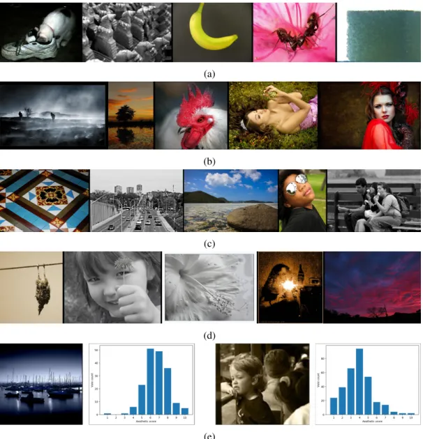
In order to study the problem of image aesthetics, one has to address the feature representation that will represent the images and the learning paradigms one will employ to infer the value of unseen images. A separate issue is acquiring appropriate datasets, since aesthetics inference is a supervised learning problem requiring aesthetic labels. The datasets can come from either of two resources: controlled studies and community-contributed resources (e.g. media-sharing net-works). Below we briefly describe the main sources where one can obtain labeled images that can be used for aesthetics inference. In Figure 2.2, we show examples of images used for aesthetics inference.
(a)
(b)
(c)
(d)
(e)
Figure 2.2: Figure showing example images from the AVA dataset that demonstrate the kind of images are used for learning aesthetic functions. We shows examples of images with (a) low mean score, (b) large mean score, (c) low standard deviation in user ratings, and (d) large standard deviation in user ratings. Part (e) show examples of high and low quality images (left and right respectively) along with their distribution of vote counts (which can be used to compute various statistics such as mean)
Flickr
Flickr is a photo-sharing platform offering a wide variety of options for editing, organizing and publishing pictures online with a vibrant community of amateur and professional photographers alike. The users can interact in a variety of ways: by following other users’ photostreams, con-gregating in Flickr Groups (often centered around common themes such as Nature photography), post comments on photographs or make a photo a ”favorite” of theirs (similar to the Like button on Facebook). Additionally, Flickr introduced a metric called ”Interestingness” which is computed for each user based on their popularity, number of favorites in receives, viewing patterns of the photo and others.
DPChallenge
DPChallenge.comgathers together a community of photographers of all skill levels, amateurs and professionals alike, who participate theme-based photography contests. Owing to its popularity, the photographs on the website are rated by a large number of people (greater than one hundred ratings per photograph) on a ten point scale and with implicit labels on the photographs provided by the contest themes, serving as a great resource for mining labeled data.
Photo.net
Photo.net was originally started at MIT in order to promote research in online communities. The users can interact by sharing, rating and commenting on the photos. Each of the photographs can be rated based on two metrics: aesthetics and originality on seven point scales. A subset of approximately twenty thousand images can be found on the website ofRittendra Datta, one of the authors of the first aesthetics papers.
Terragalleria
Terragalleria is a collection of over thirty-five thousand travel photographs taken by a single per-son. It includes a large collection on Nature photographs (e.g. US National Parks) that can be rated by the viewers on the scale from one to ten. All of the photographs are availablehere.
Aesthetic Visual Analysis (AVA) dataset.
The AVA dataset is a large collection (more than 255,000 images) collected from the DPChallenge website augmented with aesthetic (distribution of user aesthetic ratings) , semantic (sixty-six diverse textual tags describing the semantic meaning) and style annotations (labels describing various aspects and rules of thumb of photography: complementary colors, rule of thirds, etc.). The full dataset can be foundhere.
CUHKPQ
CUHKPQ was collected at the Chinese University of Hong Kong with the aim of assessing photo quality. It contains more that seventeen thousand images divided into seven semantic categories with binary labels indicating high or low quality. However, because it was created by blending high quality professional photographs with low quality images from college students, it is thought not to necessarily be representative of the real difference between high and low quality picture. Dataset itself can be found at the followinglink.
The MIRFLICKR Retrieval Evaluation
The MIRFLICKR dataset (foundhere) contains a collection of twenty-five thousand images from Flickr aiming to beopen(released under the CC License),practical(additional metadata is pro-vided in a easily accessible manner), andinteresting(only images with high interestingess mea-sure are provided). Additionally, a second version of this dataset was released containing a total of one million images and additional content-based descriptors.
One Hundred Million Creative Flickr Images (OHMCFI)
The team at Yahoo Research collected a dataset consisting of 99.3 million Flickr images and 0.7 million videos and released them under the Creative Commons licensing. Each of the pictures come with the following features pre-computed available on the AWS: SIFT, GIST, Auto Color Correlogram, Gabor Features, CEDD, Color Layout, Edge Histogram, FCTH, Fuzzy Opponent Histogram, Joint Histogram, Kaidi Features, MFCC, SACC Pitch,and Tonality. In order to request the access to the full dataset, submit a request at the followingwebsite.
Hidden Beauty of Flick Pictures
This dataset was collected as part of an effort to surface the ”hidden gems” among the pictures that have very low popularity / interestingness as measured on Flickr. Approximately 15,000 images were chosen from the sample of 9M images from the larger OHMCFI database. Although this database is not as large as the previously mentioned AVA database, it is a good starting point for aesthetics inference investigation. This is due to the fact that it is the largest database that aimed to ensure a controlled collection of the image labels. Although the labels were collected via the CrowdFlower crowdsourcing platform, each of the images was labeled by at least five different people (each evaluator having a top track record on the platform), with quality control in place, and the ratings for the pictures were clearly explained. Additionally, in order to justify the creation of the dataset, the authors benchmark the performance of the dataset against other ranking strategies and show that it outperforms all of the tested methods.
2.2.2 Handcrafted-Features
Studying computational aesthetics using a computational approach [20]
Datte et al. [20] was the first paper to tackle to problem of analyzing image aesthetics using computational techniques. They designed a set of features that would either align with princi-ples of photography and guidelines in the literature regarding psychology of aesthetics. Although the images used as data (collected from Photo.net) were rated both on their originality and per-ceived aesthetics, the study limited itself to the examination of only aesthetics scores due to strong positive correlation with originality. Because of the role color tones and saturation play in pho-tography and color psychology, the images were converted and processed in the HSV color space. The hand-crafted features were designed using the following principles: rules of thumb in photog-raphy, common intuition and observed trends in ratings. In the end, a set of 56 carefully chosen features was used to study the patterns leading to variations in aesthetic ratings. The features used in the study describe information about exposure, color, quality and composition of the image. Using all of the 56 features, they were able to achieve an overall85.9%accuracy in predicting the high / low aesthetic value of the images and thus showing possibility to study aesthetics from the point of view of statistical learning.
Design of high-level features for photo quality assessment [47]
Aiming to distinguish between high quality ”professional photographs” and low quality ”snap-shots”, Ke et al. present a top-down approach for constructing high level semantic features for photo quality assessment [47]. First the authors aimed to understand the perceptual criteria that people use to rate photos and then they distilled them to concrete measures usable as features for a machine learning algorithm.
After consultation of professional photography books and interviews with photographers and am-ateurs alike, the three distinguishing factors between the low / high quality photos come out to be:
• Simplicity simplicity in the sense that it is obvious what one should be looking at. In order to separate the subject and the background, the photographer can use the following techniques: blur the background, choosing complementary colors for the subject and the backgroundandlightning contrast between the subject and the background.
• Realism - professionals use various techniques to snap atypical photos, that almost look surreal. Since photographers often take preparation, e.g. in choosing the time of the picture and camera settings, the color palette or subject matter are likely to be much different from
snapshots.
• Basic Techniques- which might indicate the quality of the photo such as blurry image or contrast.
Once Ke et al. established understanding of what distinguishes professional photographs, they de-signed features to measure the high level perceptual factors. Simplicity is measured by computing the Spatial Distribution of Edges to understand the presence of clearly defined subject. Hue Count measured the number of unique hues in the image. Ke et al. inspected the frequency content of the image, since whole-image blur is indicative of low quality of the photograph and thus indicates ”bad technique”. Since professionals are very adept at using color to highlight the subject, the color distribution of each image is compared to that of itsk nearest neighbors. Finally, authors proposed low level features that capture contrast of the photo and its average brightness.
Learning the consensus on visual quality for next-generation image management [21]
Datta et al. proposed a novel architecture of rating images, motivated by the need to reliably retrieve high and low quality images. They proposed to exploit the available number of user ratings to estimate the consensus or degree of confidence in the estimated image quality score. Using the same features presented in [20], they trained a weighted Linear Least Squares Regressor and a Naive Bayes’ classifier to jointly predict the quality of the picture.
Photo and Video Quality Evaluation: Focusing on the Subject [72]
All of the previous approaches used feature extraction techniques on the whole image. However as the rules of composition dictate, it is important to highlight the subject of the photograph in our image. Luo et al. recognized this and detected the subject by using blur detection to distinguish clear / blurry regions. From the detected region, they extracted a variety of features including clar-ity contrast, lighting contrast, complexclar-ity, composition and color harmony. They applied the same techniques to estimating the quality of the video and define two additional features to quantify motion stability and subject presence in the video. Using these subject-focused features showed superior performance compared to [47] in Web Image Ranking, and Photo and Video Quality Assessment.
Sensation-based Photo Cropping
Automated image enhancement is of immense interest, similarly to aesthetics inference, especially because of the large collection of images each of us possess. Photo cropping, a technique in which we select a subset of the image, has mostly been accomplished by selecting regions around either
humans, by using face detectors in photographs, or the main subject as determined by saliency de-tectors. Nishiyama et al. took a data-driven approach to this problem [83]. By using SVM quality detector trained on data from DPChallenge and Photo.net (a problem very similar to aesthetics in-ference), they cropped the photos by generating several possible candidates and picking ones with the highest quality score. To train the quality classifier, a set of subject regions is extracted from the saliency map. Each region is described by an edge, color and blur histogram. Each feature is used to train a probabilistic SVM to estimate whether they are of high / low quality and in the end serve as a mid-level feature for an SVM which will determine the overall quality of the image. A study of 30 users showed the success of the technique.
Saliency-enhanced image aesthetics class prediction
Many of the rules of photography, e.g. rule of thirds, tell us ways to manipulate the subject of our image to improve the appeal of the photograph. Recognizing the importance of subjects, Wong et al. used saliency enhanced segmentation to estimate the regions of the photograph that contain the subject [115]. They used a variety of features describing texture, blur, brightness, saturation and color to describe the whole image, subjects or the contrast between the subject and the background. Using feature selection methods to pick the top performing features (primarily of the image and the subject), Wong et al. were able to outperform previous methods by>5%.
Automatic aesthetic value assessment in photographic images
Jiang et al. [41] presented a framework for estimating a continuous (0 ≤ x ≤100) and discrete aesthetic value (x∈ {1,2,3,4,5}) of image. To evaluate the framework, the authors used a previ-ously collected dataset of more than 450 images each ranked by 30 users from their earlier work on understanding the aesthetics of consumer images [12]. Cerosaletti et al. [12] analysis of the dataset in the analysis of variance (ANOVA) factors as well as the artistic characteristics revealed attributes that characterize pleasing images, however mainly the fact that degree of aesthetics and technical image quality are highly correlated.
Jiang et al. [41] extracted from each image a set of visual features explored in previous studies [20, 47]. In order to estimate the continuous aesthetic rankings, they adapted the RankBoost algorithm. Given a dataset {x1, . . . , xn}, with each xi described by a set of ranking features [f1(xi), . . . , fm(xi)], RankBoost algorithm learns a ranking functionH, which gives us a linear ordering onxi’s. By using an SVM as a weak learner in the Diff-RankBoost (DRB) algorithm, they learned to predict the relative aesthetic score between two imagesxnandxm, i.e. H(xn)−
H(xm). In order to regress the aesthetic value, the DRB algorithm is used to create a set of features
f1(xi), . . . , fn(xi)for each image xi, where fj(xi) = H(xn)−H(xm). These image features are then fed into a Support Vector Regression Machine to predict the actual targetsyn. Secondly,
the authors quantized the fine-grained aesthetic scores into five categories and trained a five-class SVM on the image features to predict these classes.
The role of image composition in image aesthetics
Image composition is one of the main determinants of image aesthetics as note by [47, 93]. Al-though often extracted features consider parts of image composition, Obrador et al. [85] were the first to do a detailed study of image composition as determinant of computational aesthetics. They described a total of 55 features that consider the image simplicity, region relevance, layout appeal and visual balance. Individually the features came short in predicting aesthetics compared to previously published methods. This might be due to the very specific nature of the features not encompassing all aspects of aesthetics. However the potential of the features became apparent when combined with previous features, which significantly improved aesthetics inference.
A Framework for Photo-quality Assessment and Enhancement Based on Visual Aesthetics
Bhattacharya et al. presented a framework for inferring and altering the aesthetics of the photo-graph [9]. The scope of the paper was limited to studying only two types of scenes: one with a single main subject and one without (e.g. landscapes and seascapes). For this study, Bhattacharya et al. assembled a dataset of 632 images and conducted user survey to rank each of the images on a five point scale. In order to learn aesthetic preference, they proposed two types of features for the different scenes that capture the composition information about the image. For single subject photos, they estimated the region of the image and estimate its center of mass or “visual attention center” using semantic segmentation. To characterize the image, they created a 4 dimensional vector with distances to the four focus points, intersection of the horizontal and vertical lines that divide the image into nine parts. For images without subject, they described each image by ratios of vertical extents of the sky and the support using the same semantic segmentation techniques. According to the rules of the composition, they should be as close to the golden ratio as possible. They learned SVR classifiers for each of the categories. In order to improve the aesthetics of the images, they proposed to relocate the subject of the image or change the ratio of sky / support by extending / cropping their regions, which resulted in improvement of estimated aesthetics in73% of the time.
Learning to Photograph
Cheng et al. used a large set of approximately105 crawled images to automatically learn the ideal rules for image quality and suggest the ideal view the photograph should take [17]. Each image was divided into a set of atomic regions using graph-based image segmentation, with each region characterized by a feature vector composed of Color Harmony and HOG texture features.
Using K-means clustering, they created a visual vocabulary of 1000 words from all of the patches extracted from images and then described each image by a Bag-of-Visual-Words. Furthermore, the images were divided into 100 sub-topics using K-means clustering and a separate probabilistic model, that models both the presence of visual words and their co-presence, was learned for each sub-topic. Using a group of fifty human subjects, they validated their model and showed its success compared to previous re-targeting models which utilized visual saliency.
High-Level Visual Attributes for predicting Visual Aesthetics
Dhar et al. developed techniques for estimating high-level describable features (kinds of char-acteristics that a human might use to describe an image) [24]. They fall intro three distinctive categories:
• compositional attributes- characteristic related to the layout of an image that indicate how closely an image follows photographic rules of composition
• content attributes- characteristics related to the presence of specific objects or categories of objects including faces, animals, and scene types.
• sky-illumination attributes- characteristics of the natural illumination present in the pho-tograph.
For Dhat et al., describability of the attributes was essential, as group of people can be queried regarding the presence and absence of such attributes. This data was then used to train classifiers to predict these attributes and estimate aesthetic value / interestingness of images. The research built upon work on face recognition, where face attributes, e.g. race and gender, were shown to improve facial recognition results. One of the main contributions of the paper was showing that by training classifier to estimate the describable attributes and then using these attributes as features can significantly improve the prediction of the aesthetics and interestingness scores.
A total of 26 classifiers indicating the presence of above features was trained on hand-labeled data collected from: Flickr, Photo.net and Animals on the Web dataset. In order to estimate the aesthetics and interestingness, additional sets of sixteen and forty thousand images were collected on DPChallenge.com and Flickr, respectively. The top 10 % of images were labeled as high aesthetic quality / interestingness value and bottom 10 % of the images were used to denote the negative examples. Dhar et al. trained an SVM classifier using the 26 describable features and demonstrated effectiveness in measuring both. In each case, the SVM classifier trained on high-level features outperformed a baseline Naive Bayes classifier by Ke et al. trained on low-high-level features. The classifier performance was further improved by combining both high-level attributes and low-level features.
Aesthetic Quality Classification of Photographs Based on Color Harmony [82]
Previous papers recognized the importance of color in aesthetics inference. This was especially due to the evidence from study of psychology and art theory, which showed that color often in-duces different emotion in people. Nishiyama et at. [82] pointed out that previous papers used rather simple descriptors of color, e.g. average values of the RGB channels, or color histogram. Nishiyama et al. proposed a new set of features, ’bag-of-color-patterns’, which aimed to charac-terize the color harmony of the photograph.
Color harmony is a property certain combinations of color are said to have if they together have an aesthetically pleasing effect on the observer. Otherwise, non-harmonious combination of color would not engage the observer or make them look away from the picture, in the case of chaotic colors [79]. Color Harmony is mainly discussed by two models: The Moon-Spencer model and the Matsuda methods. These models have been used in variety of applications to design harmonious color combinations, e.g. marketing campaigns, website design, clothing pattern design. They cannot however be used to describe the color harmony of a picture, whose spatial color pattern is much more complicated than that of a simple dress design.
In order to describe the harmony of the image, the authors proposed to sample smaller patches of the image where each region ends up having a simpler combination of colors. Then one can use color harmony models to describe each of the patches, which are then combined to a descriptor of color harmony in the image. In their algorithm, authors sampled the image on a uniform grid, div-ing the sampled regions into uniform and ones with color edges. Each region was then described by a color histogram in the CIE LCH color space. To create the bag-of-color-patches features, a large number of local patches was sampled from the images in the training set and codebooks for the regions with / without color edges were created using k-means clustering. Lastly, each image was divided into several larger regions, each described with a histogram of local image patches which are then concatenated to create a representation of the whole image. Combining the bag-of-color-patches histogram, with blur, saliency and edge features showed superior performance of such methods outperforming the competing models by a large margin.
Content aware aesthetics
The purpose behind or the type of the photograph the author is trying to take is going dictate many of the choices of the photographer: if they aim to capture a particular subject, e.g. an animal, a plant or an insect, they are likely to choose a blurry background to focus our attention. Otherwise, if they take the picture of a person, we will naturally be drawn towards a human face. This is indicative of the fact that different photo categories would require distinctive mix of features to recognize the its quality.
Tang et al. were one of the first works to explicitly consider photo content in [71, 100]. They collected a dataset consisting of seven photo categories and computed two types of features: global (computed on the whole image), and local (computed on the subject of the image).
To estimate the subject of the image, they considered three different subject area extraction techniques for the different categories. The subject area for:
• ”animal”, ”static”, ”plant” and ”night” categories was extracted by estimating the blur in the image.
• ”architecture” and ”landscape” was estimated by extracting vertical standing objects from a previously published scene segmentation algorithm.
• ”human” was estimated using face / human detection algorithm.
In order to evaluate the subject areas of the images, the proposed the following regional features: 1. Dark Channel Feature - average normalized dark channel value (described in [32]).
2. Clarity Contrast - aims to capture the sharpness of the subject areas by comparing the fre-quency content in the subject and the whole image.
3. Lighting Contrast - compares the average lighting between the subject and the background. 4. Composition Geometry - measures the Rule of Thirds by computing the minimum distance to one of the four image intersections (as defined by the two horizontal / vertical lines diving image into nine regions).
5. Complexity Features - aims to capture the complexity of the image by counting the super-pixels the background / subject is segmented into.
6. Human Based Features - aims to capture the quality of portraits by considering the ratio of face area in the image, amount of shadow in the faces, average lighting of the faces, and their clarity.
To capture the information about the image, the authors extracted:
• Hue Composition Feature - which aims to capture the color harmony of the image by con-sidering where the majority of hues values cluster on the color wheel.
• Scene Composition - by using the Hough Transform to extract the horizontal and vertical lines in the image, they aim to capture the average position of orientation of these lines. Tang et al. treated the scene categories as ground truth. To solve the problem of estimating the image category, they proposed the following method:
• compute the Edge Orientation Histograms, HOG and GIST features.
• retrieve the top 100 high / low quality nearest neighbors from the training data.
• using the training labels, estimate which of the subject extraction techniques is to be used • train a linear SVM based on the retrieved training samples to estimate the class of the test
sample.
Tang et al. noted their features outperformed their benchmarks, though they did not compare their results to any features / algorithms that were published recently in their time frame, e.g. the color harmony features described in the previous section.
Obrador et al. [84] took a similar to approach and introduced their own dataset collected at DPchal-lenge.com. They computed three categories of features:
• Simplicity features - quantified by measuring various statistics about the regions of graph-based segmentation algorithm.
• Global features - 38 low level features capturing information about the luminance, contrast, colorfulness, color harmony, and composition (e.g. rule of thirds) of the image.
• Contrasting features - by using sharpness, luminance, chroma, relevance and saliency, they create five binary maps that classify the image into subject / background and compute vari-ous low level features that measure sharpness, exposure, chroma and saliency of the regions. Contrary to most of the models, Obrador et al. trained a SVM regressor to predict the real valued scores, instead of binarizing the scores. After computing all of the features for the training images, they used feature selection methods to obtain the set of best performing features for each of the categories and demonstrated the improvement in aesthetics score prediction for category specific models as opposed to the generic model.
2.2.3 Local Features
Zhang et al. [120] proposed a graph-based probabilistic approach for aesthetics inference which aimed to capture both local and global image information. In their approach, they segmented the image into several ’atomic’ regions using unsupervised fuzzy clustering, forming a graph G= (V, E).V is the set of vertices each corresponding to the atomic regions of the image endE
is the edge set representing the adjacent regions in the image. Each region was represented by a three sets of visual features: HOG (128-d), Color moment (9-d) and visual saliency features (64-d). For each image, a set of five hundred graphlets, connected induced subgraphs, was sampled with each of maximum size T (to be specified by the user). A t-vertex graphlet was represented
by four matrices: MRC, MRT, MRSandMS. MRC ∈Rt×9, where each row is a 9-d color vector for each of the regions in the graphlet (MRC, MRCare defined identically).MSaims to capture the local structure of the connections between the t regions, very similar to a adjacency matrix. Then all of these features were concatenated into three matrices{MC, MT, MS}, whereMC = [MRC, MS]. The authors proposed a manifold embedding, which was used to transform the different sized matrices into fixedd-dimensional vectors and encodes the global spatial layout into the graphlets as well. Once all of the graphlets (for test and train images) were transformed into post-embedding graphlets, they were used in a probabilistic graphical model to computeγ(I∗) =p(I∗|I1, . . . , IH). As the authors noted: γ(I∗)can roughly be interpreted as the ”amount of graphlets that can be transferred from the training photos into the test one”. They demonstrated the efficacy of the algorithm by comparing the algorithm on three datasets against five different feature extraction methods and achieving state of the art results.
2.2.4 High-level Features
By using the CNNs, one can automatically discover the features as opposed to using : • handcrafted features, which are merely approximation to photographic rules, • generic features.
One of the main advantages of using hand crafted or generic-features is that they compute a fixed representation of the picture, the same number of features for each image. Thus it is easy to take the features and feed them into a learning algorithm. However, applying CNNs can at times prove to be tricky, since NNs take a fixed input as well and images often come in various aspect rations and sizes.
Lu et al. [68] were among the first to tackle the problem of aesthetics inference that solely uses CNNs. They conducted a thorough study of several network architectures and experimented with constructing a multiple column network with varying inputs. As different photographic rules (e.g. rule of thirds or color harmony) consider properties on different scales of the image, authors used both the global and the local view (random fixed crops) of the image to train the networks. To get around the problem of varying image sizes, following image transformations to fix the size of the image tos×s×3were proposed:
• Center-crop- resize the shorted side of the image to a fixed sizesand take the ”center”s
pixels to form the image
• Padding- resize the longer side of the image to a fixed sizesand padding the rest of the image with zeros.
Since the global and local details of the image are important, the authors proposed a Double Col-umn CNN (DCNN), where one of the colCol-umns accepts a global-view of the image and the other a local-view. It was essentially a network consisting of two separate Single Column CNN (SCNN) whose outputs were combined to produce a single score. Because of the large intra-class variation in aesthetics scores, Lu et al. proposed to use higher-level style labels, that are available for a subset of images present in AVA dataset, as additional features. They trained an additional Style SCNN to recognize the various style labels (e.g. complementary colors, motion blur or the rule of thirds). The trained network was then used to extract the Style features for the rest of the images in the AVA dataset. These features were then concatenated with the features computed by the DCNN network and used to determine the final aesthetics score. A very interesting detail arose when looking at the images correctly classified by the DCNN and incorrectly by SCNN: when the input was a local-view of the image, it often contained a large subject and similarly when the input was a global-view, the image often contained specific texture likely to be better seen on the local-view. Wang et al. took inspiration from Neuroaethetics and Neuroscience of Vision to propose a novel architecture that aimed to tackle the problem of binary classification and the distribution of aes-thetics scores [108]. They proposed a model called the Brain-Inspired Deep Network (BDN) composed of two parts:
• Parallel Pathways layer • High-level Synthesis Network
TheParallel Pathways layerwas inspired by the parallel pathway processing of the human cortex, which decomposes the visual scene into several representations that encode information such as intensity and edge information in the image. In this layer they converted the RGB data into the HSV format and used each H, S, V as one of the parallel representations for the image. As was shown previously in [24], high-level attributes are successful in augmenting aesthetics prediction if used as mid-level features. Therefore Wang et al. decided to train fourteen fully-convolutional networks (FCN) trained in a supervised ways to predict the fourteen binary style labels available with the AVA dataset. The activation of the mid-level convolutional networks for each of the four-teen style label were used in parallel as features for the high level synthesis network (thus virtually decomposing image into several representations encoding different information). The synthesis network, also a FCN, was used to predict the binary high / low aesthetic label as well as the dis-tribution of ratings (by predicting the mean and deviation of a Gaussian disdis-tribution trained by minimizing the Kullback-Leibler divergence).
Guo et al. [29] proposed to use paralleled Deep CNN (PDCNN) architecture. They utilized an ar-chitecture similar to the AlexNet that won the 2012 ImageNet Competition [55]. Since the CNNs are prone to both over- and under-fitting, they proposed to use PDCNN to control the complexity of the system by stacking n columns in parallel - n-PDCNN. As they showed, the performance of the network network improved when they stacked up to three networks in parallel. Thereafter, with more then four paralleled inputs the performance started to degrade.
Kong et al. [53] proposed AlexNet-inspired architecture to predict various image attributes. First, they created a simple regression network to predict aesthetic rating by minimizing the Euclidean loss. Subsequently, they adopted a Siamese Network architecture [11] to jointly optimize the network to both predict an aesthetic score and a relative ranking of the two images. Similar to [108], Kong et al. predicted the aesthetic attributes of images augmenting the network with an auxiliary task of predicting attributes from the same activations that were used to predict the aesthetic score. Lastly, the network was used to predict image categories.
2.2.5 Related Work
What makes images pleasing ?
Marchesotti et al. set out to discover sets of textual image attributes that could be used a mid-level features for various tasks, including image ranking or aesthetics prediction [70, 76]. They used the AVA dataset [80], which along with images, their aesthetic scores and style labels, contains com-ments associated with each of the images. The comcom-ments were used to construct Bag-of-Words feature vectors (using tf-idf (term frequency-inverse document frequency) feature representation for the words) for each of the images and used the elastic net model (a linear combination ofl1
andl2regularization) to discover attributes most predictive of beautiful / ugly pictures. They used
both unigrams and bigrams, and found that bigrams were much more suitable as attributes since unigrams often yielded ambiguous descriptions (“not”, “out”, , “don’t”). They picked the top 1500 ugly and beautiful attributes and used spectral clustering to reduce the number of total labels to 200 (using the Levensthein word similarity measure to gauge the similarity of the second word, since it is the one thought to contain the actual semantics with the first word bearing the polarity of the attribute, e.g. great lighting). Then they used images with the discovered attributes to train one-vs-all classifier to use them to describe images using features that are actually human interpretable. Majority of the work done is formulated as either a classification or regression problem with the goal of predicting a single aesthetic judgement / score that tells us how appealing the image is. However it often does not explain what makes the image appealing or not. When designing most of the aesthetic inference algorithms, many of the features (numbers that we compute to represent various information about the image) are solely chosen for their ability to improve the algorithm
(in terms of classification accuracy or RMSE score). Aydin et al. [6] set out to remedy this issue and defined a set of image attributes one would quantify and would be related to photographic principles, thus help us guide in taking better pictures and provide an objective basis for compar-ing their aesthetic appeal.
In order to choose what photographic principles to capture in their aesthetic attributes, the authors chose the following criteria that the attributes should satisfy:
• Generality- e.g sharpness, which can be used to judge every image versus an attribute such as facial expression
• Relation to photographic rules
• Clear definition
The attributes that were in the end chosen by the authors were:
1. Sharpness- aims to capture the level of detail seen in the in-focus region.
2. Depth- aims to capture the impression of ”depth” in the picture, which can for example be created by blurring the background of the image.
3. Clarityaims to capture whether the photograph or image has a clear principal idea, topic, or center of interest.
4. Toneis related to the magnitude of the global lightness differences.
5. Colorfulness- as discussed previously, pictures with a vibrant color palette are often con-sidered to be more aesthetically pleasing.
By defining, computing and calibrating (making sure the actual output values have equal ranges), the authors presented a framework that computes an aesthetic signature of the image, compris-ing of measures of visual image attributes that relate to specific photographic principles. They demonstrated the performance of the ratings by exploring several possible applications such as:
• Automated Aesthetic Analysis • Photo editing evaluation • HDR Tone Mapping Evaluation • Multi-Scale Contrast Editing
Image ranking and retrieval
Image ranking is a problem of great importance, especially to image search engines which aim to index the content of the web and then serve it to the user at their will. When retrieving the images for a given query, the images that are shown should take into account three main aspect: semantic relevance, quality and variety of images [44]. The quality of the images can be quantified by various metrics: popularity among images on a social networking website like Flickr or aesthetics value computed using an algorithm.
Multidimensional Image Value Assessment and Rating for Automated Albuming and Re-trieval [66]
Loui et al. [66] proposed a multidimensional image value index (IVI) to be used by an automated system for raking of images. It comprises a signature of a photo that captures various higher level information about it: its quality, aesthetics as well as relevant semantic value to the user. M-IVI comprises of five IVI values: Technical, Aesthetic, Social, Event and Usage. The authors proposed to learn the Technical IVI in a data-driven way. On the contrary, the social IVI was determined in more heuristic / manual definition of some of the values, since it tries to capture the personal relevance of the people in the photographs to the user. Loui et al. demonstrated the feasibility of implementing the Social and Technical IVI, however more work would have to be put in to adequately define rest of the values. This was due to the fact since the meaning they tried to capture either requires a lot of additional user input (not always desired or easily available) or implementation of a complicated system that combines face detection, metadata, etc.
Marchesotti et al. [81] described an algorithm that aims to augment the image retrieval system by ranking the images not only according to their semantic relevance to the query, but also aiming to ensure that the images are aesthetically pleasing. They first introduced a previously published algorithm from an earlier paper that learned a joint model that will take into account both seman-tics and aestheseman-tics. [81] however demonstrated that learning separate models for semanseman-tics and aesthetics provides much better performance in ranking. They proposed the following two models: • Independent Ranking Model- assumes that aesthetics and semantics are separate given
image:
p(y, z|x) =p(y|x)p(z|x)
• Depender Ranking Model- assumes that aesthetics is going to be dependent on the se-mantics of the image:
p(y, z|x) =p(y|x)p(z|y, x)
As they demonstrated in the metrics, both of these models outperformed the original model, which aimed tries to learn a joint model.
(a) Artificial neuron (b) Elementary neural network (c) Local connectivity of a neuron.
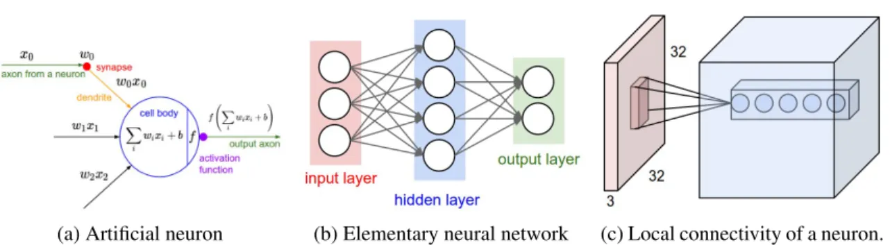
Figure 2.3: Figures showing (a) model of the neuron used in neural networks, (b) architecture of an elementary neural network with a single hidden layer, and (c) the local connectivity of a neuron in a convolutional layer. Source: https://cs231n.github.io/
2.3
Neural Networks and Deep Learning
In this section we briefly discuss neural networks, which currently dominate the approaches in several areas of computer vision, e.g. object detection and classification, face detection or speech recognition. We discuss backpropagation, a method of optimizing weights of a neural network, a basic model of a neural network, and lastly ranking optimization that is utilized in Chapters 5 and 6 of this thesis.
2.3.1 Backpropagation
Backpropagation is a particular method of computing the gradients of the loss / error function with respect to the parameters, using the multivariable chain rule, by considering the loss tion as being a composition of several nonlinear functions. For example, consider the func-tion f(g(x(t), y(t))). In order to backpropagate the gradient, we first find ∂f∂g. Then we have ∂f ∂x = ∂f ∂g ∂g ∂xand ∂f ∂y = ∂f ∂g ∂g
∂y. In the end, we have ∂f ∂t = ∂f ∂x ∂x ∂t + ∂f ∂y ∂y
∂t.Similarly, the gradient of the loss function with respect to weights is calculated by backpropagating the error through the different layers of the neural network. Once the gradient is computed with respect to all of the parameters, stochastic gradient descent [114] (or a variation of it) is used to update their value. The value of parameterwat stepn+ 1would thus be updated as follows:
w(n+1)=w(n)−α∂L ∂w.
2.3.2 Neuron function
Figure 2.3a shows the model of an artificial neuron that approximates the function of real neuron with all of its parts: synapse, dendrite, cell body and axon. The inputs,x1, . . . , xninto neurons are represented as signals traveling through dendrites, whose effect is modulated by the synaptic weightwi. The effect from all of the weighted inputs is then summed together and biased with a bias termb. The sum is then transformed via a nonlinear function (paralleling the neuronal firing of a neuron) and the output travels along an ”axon” and serves as an input into further neurons. As can be seen in Figure 2.3a, the output of the neuron can be written as:
y=f(X i
wixi+b) =f(xTw).
In the above equation, the bias termbwas absorbed as a weightw0 withx0 = 1
2.3.3 Neural Network
This section describes a basics of neural networks, and describes equations for a 2 layers feed-forward neural network for classification, using the softmax loss function, seen in Figure 2.3b, which can then be extended into more complicated models, e.g. the convolutional neural network. The following variables be of interest:
• N - number of inputs processed at the same time • D - number of input dimensions
• H - number of hidden units (neurons) • K - number of classes for classification
Additional notation has to be introduced. Since each of the neurons in the hidden layer is fully connected to all of the inputs, each neuron will have a separate synaptic weight modulating the input differently. Thus letwi,j represent the weight modulating theith input for thejth hidden neuron. We can store all of the weight conveniently in a weight matrixW:
W=
wi,j
In our network, we will need two weighting matrices:W(1)transforming the inputs to activation of hidden layer neurons andW(2) transforming neuron outputs to theK class scores. The inputs are going to be stored in matrixX, wherex(in)is theithinput feature of thenthexample.
X=
h
x(in)
i
Therefore starting with an example matrixXand weight matrixW(1), the transformed outputs
of the neurons are found as follows:
H=f
X·W(1)
,
where·represent matrix multiplication andf(·)represented element-wise application of the rec-tified linear unit (ReLU) nonlinearity [55]:
f(x) =
x , if x>0 0 , otherwise
Furthermore,K, the matrix of class scores for the all of the examples are calculated: K=H·W(2),
where each elementfk(n) represents the score indicating the belief that thenthexample belongs tokthclass. To make these notions more clear, we will convert the class scores into probabilities using the normalized exponential function also known as softmax [113]:
p(kn)= e fk(n) P ief (n) i
Since we are performing supervised classification, each data pointx(n) is accompanied by a cor-responding class labelyn ∈ {1, . . . , K}. The loss function to be optimized for each example is the softmax loss function:
Li =−log(p(yii)), and the total loss for all of the examples is defined as follows:
L= 1 N X i Li | {z } Data Loss +X i X j w(1)i,j 2 +X i X j wi,j(2) 2 | {z } Regularization Loss
Function L can be further viewed as a composite function of the network parameters, and thus we can use backpropagation to optimize the network weights to minimize its functional value to improve performance of the model. Using the chain rule, we can show that:
∂L ∂fk(n) = 1 N ∂Ln ∂fk(n) = 1 N 1 p(kn) ∂ ∂fk(n) (p(kn)) ! = 1 N h p(kn)−1(k=yn) i .
Let∂Lrepresent the matrix of partial derivatives with respect tofk(n). Furthermore, we would like to find ∂W∂L(1) and
∂L
∂W(2). Note, that for
∂L
∂W(1), we will have to back-propagate the error through the hidden units as described in the previous section. Thus first, consider ∂L
∂w(2)i,j (temporarily omit
λw(2)i,j from the regularization loss):
∂L ∂w(2)i,j =X n ∂L(n) ∂wi,j(2) =X n ∂L(n) ∂fj(n) ∂fj(n) ∂w(2)i,j =X n ∂L(n) ∂fj(n) a(in)=aTi ·∂Lj,
whereaiis the column vector ofithhidden layer neuron activations and∂Ljis thejthcolumn of
∂L. Since ∂L ∂wi,j(2) =a
T
i ·∂Lj, we can see that ∂W∂L(2) simply is:
∂L
∂W(2) =H
T ·∂L+λW(2).
To propagate the error back to earlier layers, it is necessary to compute ∂L ∂a(in): ∂L ∂a(in) =X k ∂L ∂fk(n) ∂fk(n) ∂a(in) =X k ∂L ∂fk(n) w(2)i,k =∂L(n)·w(2)i, T ,
where∂L(n) is the nth row of ∂Landw(2)i, is the ith row ofW(2). Form of ∂L
∂a(in) = ∂L
(n)·
w(2)i,
T
hints at the fact that∂H can simply be computer as:
∂H =∂L·W(2)
![Figure 3.8: Benchmarks. Performance of the various algorithms on the ImgSal [63] dataset.](https://thumb-us.123doks.com/thumbv2/123dok_us/1296375.2673724/53.918.301.719.639.971/figure-benchmarks-performance-various-algorithms-imgsal-dataset.webp)
![Figure 3.9: Benchmarks. Performance of the various algorithms on the SED1 [4] dataset.](https://thumb-us.123doks.com/thumbv2/123dok_us/1296375.2673724/54.918.301.720.190.524/figure-benchmarks-performance-various-algorithms-sed-dataset.webp)