DeepFGSS: Anomalous Pattern Detection using Deep Learning

(1)

DeepFGSS: Anomalous Pattern Detection using Deep

Learning

A THESIS

SUBMITTED TO THE FACULTY OF THE GRADUATE SCHOOL OF THE UNIVERSITY OF MINNESOTA

BY

Akash Kulkarni

IN PARTIAL FULFILLMENT OF THE REQUIREMENTS FOR THE DEGREE OF

MASTER OF SCIENCE

Edward McFowland III

(2)

c

(3)

Acknowledgements

Firstly, I would like to thank my adviser, Prof. Edward McFowland III for his guidance, mentorship and bringing out the researcher in me.

I would also like to thank my thesis committee members, Prof. Vipin Kumar and Prof. Erika Helgeson for providing their valuable feedback on my thesis.

Finally, I would like to thank my parents for their constant love, my friends for their un-wavering support and encouragement and my brother, Vishal, for pushing me to pursue masters abroad.

(4)

Dedication

To my mom, dad and best buddy, Anurag Kakati.

(5)

Abstract

Anomaly detection refers to finding observations which do not conform to expected behavior. It is widely applied in many domains such as image processing, fraud detec-tion, intrusion detecdetec-tion, medical health, etc. However, most of the anomaly detection techniques focus on detecting a single anomalous instance. Such techniques fail when there is only a slight difference between the anomalous instance and a non-anomalous instance. Various collective anomaly detection techniques (based on clustering, deep learning, etc) have been developed that determine whether a group of records form an anomaly even though they are only slightly anomalous instances. However, they do not provide any information about the attributes that make the group anomalous. In other words, they are focussed only on detecting records that are collectively anomalous and are not able to detect anomalous patterns in general. FGSS [45] is a scalable anomalous pattern detection technique that searches over both records and attributes. However, FGSS has several limitations preventing it from functioning on continuous, unstructured and high dimensional data such as images, etc. We propose a general framework called DeepFGSS, which uses Autoencoder, enabling it to operate on any kind of data. We evaluate its performance using four experiments on both structured and unstructured data to determine its accuracy of detecting anomalies and efficiency of distinguishing between datasets containing anomalies and ones that do not.

(6)

4.6 DeepFGSS Algorithm . . . 32 4.7 Computational Complexity . . . 33 5 Evaluations 35 5.1 Experiments . . . 35 5.1.1 Power curve . . . 35 5.1.2 ROC curve . . . 36 5.1.3 Jaccard curve . . . 37 5.1.4 Precision-Recall curve . . . 38 5.2 Datasets . . . 39 5.2.1 Network Intrusion . . . 39 5.2.2 Handwritten Digits . . . 42

6 Conclusion and Discussion 50

References 52

Appendix A. Precision-Recall Plots for KDD Dataset: Apache2 59

Appendix B. Precision-Recall Plots for KDD Dataset: Neptune 62

Appendix C. Precision-Recall Plots for MNIST Dataset 65

(8)

List of Tables

3.1 Four cases for BN learning problems . . . 16

(9)

List of Figures

2.1 Collective anomaly corresponding to an Atrial Premature Contraction in an human ECG output . . . 6 2.2 Collective anomaly corresponding to an Atrial Premature Contraction in

an human ECG output . . . 7 3.1 Illustration of software run completion using Bayesian Network . . . 16 3.2 Autoencoder with one hidden layer illustrating its two components:

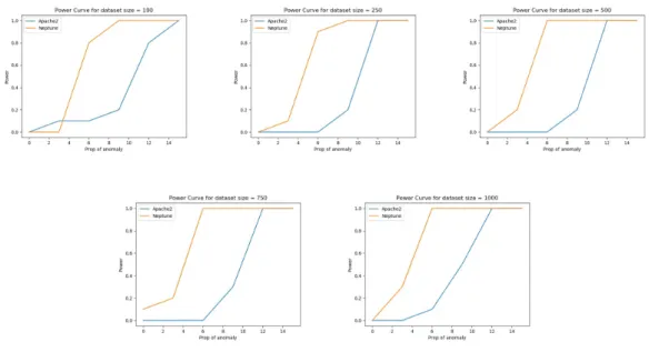
en-coder and deen-coder . . . 19 5.1 Power curves for KDD dataset for two types of anomalies: Apache2 and

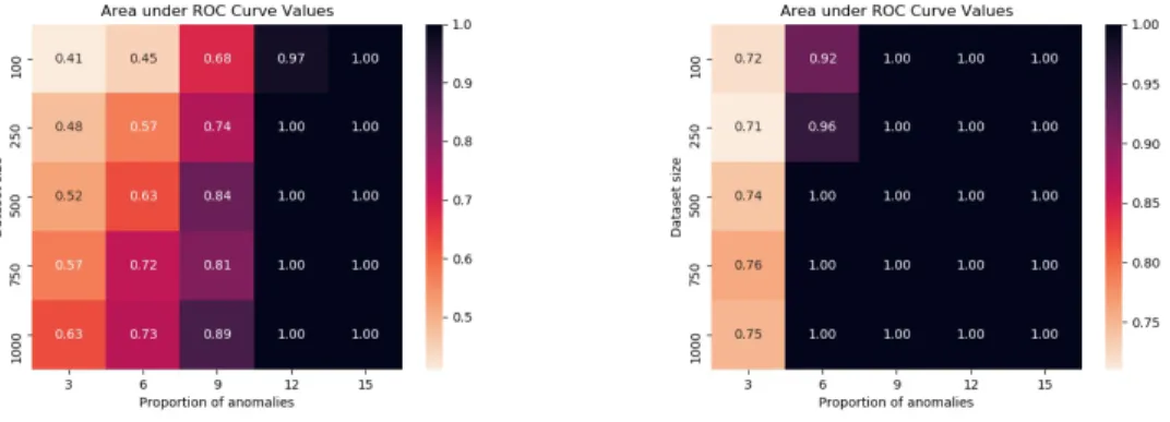
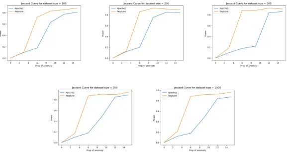
Neptune . . . 40 5.2 Area under ROC for Apache2 . . . 41 5.3 Area under ROC for Neptune . . . 41 5.4 Jaccard curves for KDD dataset for two types of anomalies: Apache2 and

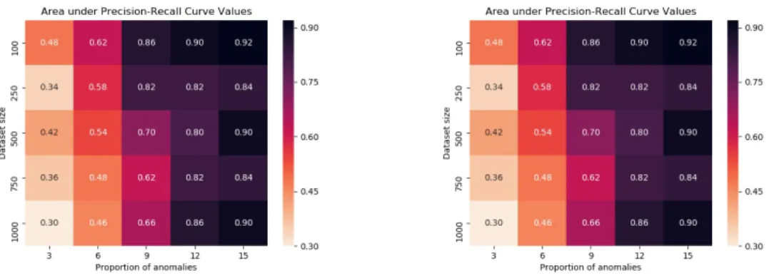
Neptune . . . 42 5.5 Precision-Recall curves for KDD dataset with N=1000 and Apache2 anomaly 43 5.6 Precision-Recall curves for KDD dataset with N=1000 and Neptune anomaly 44 5.7 Area under Precision-Recall curve for Apache2 . . . 45 5.8 Area under Precision-Recall curve for Neptune . . . 45 5.9 Power curves for MNIST dataset . . . 46 5.10 Area under ROC curve for MNIST dataset with different dataset size and

proportion of anomalies . . . 47 5.11 Jaccard curves for MNIST dataset . . . 48 5.12 Precision-Recall curves for MNIST dataset for N=1000 . . . 48 5.13 Area under Precision-Recall curve for MNIST dataset with different dataset

size and proportion of anomalies . . . 49

(10)

A.2 Precision-Recall curves for KDD dataset with N=250 and Apache2 anomaly 60 A.3 Precision-Recall curves for KDD dataset with N=500 and Apache2 anomaly 60 A.4 Precision-Recall curves for KDD dataset with N=750 and Apache2 anomaly 61 B.1 Precision-Recall curves for KDD dataset with N=100 and Neptune anomaly 62 B.2 Precision-Recall curves for KDD dataset with N=250 and Neptune anomaly 63 B.3 Precision-Recall curves for KDD dataset with N=500 and Neptune anomaly 63 B.4 Precision-Recall curves for KDD dataset with N=750 and Neptune anomaly 64

C.1 Precision-Recall curves for MNIST dataset for N=100 . . . 65

(11)

Chapter 1

Introduction

Any data instance is considered to be an anomaly if its characteristics deviate from what is considered normal, expected or standard. Such deviations can be outliers, or an exception, or a novel instance, or some contaminant or simply noise. Hence, the purpose of detecting anomalies can be outlier detection, noise removal, or sometimes detecting interesting patterns. Generally, anomaly detection refers to the problem of finding any pattern in data that does not conform to expected behavior. Anomaly detection is significantly used in applications such as banking systems, health care, cyber-security, military surveillance for enemy activities and other safety-critical systems.

Usually, anomalies are recognized as harmful deviations. For example, as mentioned previously, detecting fraudulent transaction in bank statements, detecting a tumor in MRI, detecting unusual network traffic and so on. However, anomalies do not necessarily have to be bad either. For example, for an advertisement company getting Rate Of Interest exceedingly high for this month compared to the gain from previous months is a good sign.

Irrespective of whether an anomaly is harmful or not, techniques used for detecting such aberrations are the same. Over time, there have been various techniques developed which work on different principles and assumptions. Most of the techniques developed so far focuss on detecting point anomalies. In the next section, we will explain what are point anomalies along with techniques to detect them followed by limitations of such techniques.

(12)

1.1 Point Anomaly Detection

Point anomaly is an anomaly when a single data instance is anomalous. Chandola, Banerjee, and Kumar [11] provided an exhaustive categorization of anomaly detection techniques and their assumptions and principles.

Classification based anomaly detection techniques are supervised. First, a model is trained on the training dataset to classify a data instance. Then, the model classifies the data instance into anomalous or normal class. Examples of such machine learning techniques are logistic regression, SVM, etc.

Nearest neighbor based anomaly detection techniques, first, calculate the neighbor-hood of the data instance based on some distance metric (for eg, Euclidean distance for continuous attributes, matching the coefficient for categorical attributes, etc) and then, label data instances falling in the dense neighborhood as normal and those far from their nearest neighbor as anomalies. Examples of such techniques can be K-Nearest Neighbor (KNN), or intelligent data structures such as k-d trees, etc.

Anomaly detection techniques based on clustering work on different principles:-Density-Based Spatial Clustering of Applications with Noise (DBSCAN)[28], Shared Nearest Neighbor (SNN) [27], WaveClustering [58]- classifies those data instances as anomalies which do not belong to any cluster; Self Organizing Map (SOM) [65], K-means clustering, Expectation Maximization labels those data instances as anomalies that are far from the centroid of their nearest cluster; Cluster-Based Local Outlier Fac-tor(CBLOF) [35], CDtrees [61] labels those data instances as anomalous which belong to a cluster which is either small or sparse.

Statistical anomaly detection techniques learn a model which can generate the data seen in the training dataset and then statistical inference test is applied to determine if a given test instance is an anomaly or not based on whether it occurs in a high probabilistic regions or low. These can be parametric such as Gaussian-based model like Z-score or extreme value analysis [59], or non-parametric techniques (such as histogram based outlier score[32], Generative Adversarial Networks [33], etc).

(13)

3

1.2 Limitations

These anomaly detection methods focus on the identification of a single anomalous data record. For example, detecting a fraudulent transaction in financial data, detecting a system malfunction while analyzing system log files, detecting bots that generate fake reviews on social media platform, detecting energy leakage in smart houses or detecting excessive power utilization in data centers, etc. Some of the anomaly detection techniques devised are also domain specific, making them hard to adapt to a different problem.

However, in the real world, sometimes it’s hard to detect anomalous behavior where each individual data instance can be slightly anomalous making it difficult for anomaly detection techniques to be effective, mentioned in the previous section, to detect. For example, in the case of detecting fraudulent transactions in financial data, an intelligent fraudster will attempt to disguise their activity so that it closely resembles legitimate transactions making each fraudulent transaction only slightly anomalous. This makes the situation worse to discern the malign activity. Similarly, an intelligent hacker might also try to mimic normal network activity while sniffing data. In the case of customs officials responsible for detecting smuggled items, they must decide which shipments to inspect. An intelligent smuggler would intelligently sneak in contrabands by making similar illegal shipments - let’s say, with same declared contents on the contraband, shipping through the same company name, to the same port.

In such cases, classification techniques will not be able to learn a clear decision boundary between normal and anomalous instances. Nearest neighbor based techniques also fail to detect such anomalies as the records are only slightly anomalous and hence might fall into a denser region with other normal instances. Clustering based techniques might also fail as anomalous instances which almost resemble normal instances might not be farther from the centroid of the cluster or anomalous instances might themselves be part of a larger cluster. Traditional statistical techniques will also not be able to distinguish slightly anomalous instances because they might not necessarily fall in a region with low probability density.

One way to detect such anomalous behaviors is by searching for groups of these similar data instances each of which is only slightly anomalous. Such anomalies are

(14)

called collective anomalies whereas all the previous anomaly detection techniques aim for detecting point anomalies (where a single data point in a dataset is sufficiently anomalous)

(15)

Chapter 2

Collective Anomaly Detection

Collective anomaly is defined as a collection of related data instances that are anoma-lous compared to the entire data set but individual data instances may not be anomalies themselves. For example, in a UDP flooding attack in the network domain, the attacker sends multiple concurrent UDP packets which causes the host application to throttle and reply with an ICMP destination unreachable packet. This event overloads the host machine and renders it inaccessible. A single UDP packet sent on a port is not an anomalous event. However, when their frequency exceeds a certain level, it be-comes collectively anomalous. Figure 2.2 illustrates a famous example [11] of a human electrocardiogram output with a small region being highlighted in red which denotes a collective anomaly. Note that the low value of ECG itself is not an indication of abnormal behavior.

2.1 Background

The survey by Chandola, Banerjee, and Kumar [11] provides an exhaustive survey of various collective anomaly detection techniques developed until 2009. Collective anoma-lies majorly have two kinds of relations: sequential and spatial. Some techniques [9] convert the sequences into a finite set of features and run a point anomaly detection algorithm. One challenge in such methods is that the sequences can be of variable length. One of the techniques to overcome that challenge is box-modeling [10] which maps each term in the sequence to one of the boxes based on its value and use those

(16)

Figure 2.1: Collective anomaly corresponding to an Atrial Premature Contraction in an human ECG output

boxes as a set of features to use any of the point anomaly detection techniques. Re-cently, deep learning based techniques have also been developed to detect anomalous sequences with variable length. One such technique utilizes Long Short Term Memory RNNs [7] which predicts several time steps ahead of the input. If the prediction error is greater than some threshold for a given number of time steps, it indicates that the most recent sequence is a collective anomaly. Several clustering based techniques [8] have also been developed with similarity metric such as longest common subsequence, etc. to detect collective anomalies as a cluster. NKICAD algorithm [3] is another clus-tering based algorithm which first runsx-means algorithm [49] and then the features of the data are aggregated to form a new set of features and each cluster is re-clustered. The cluster with the minimum variance is returned as a collective anomaly. Informa-tion theoretic based co-clustering technique [2] has also been developed which return the largest row cluster as the candidate collective anomalies. Hurst Parameter based Collective Anomaly Detection (HCADET) [1] is a method which first runs x-means clustering on the entire dataset and then sorts the clusters based on their H [14] value and returns top-η clusters as a set of collective anomaly candidates.

(17)

7

Figure 2.2: Collective anomaly corresponding to an Atrial Premature Contraction in an human ECG output

data. However, these techniques do not provide any insights about the attributes which are anomalous with respect to normal data.

In the next section, we will explain three techniques which can detect both anomalous records and attributes (called as anomalous patterns) along with their limitations.

2.2 Detection of Anomalous Patterns

2.2.1 Problem Statement

Anomalous Pattern Detection is slightly different from anomaly detection. Instead of identifying individual anomalies, the aim is to identify a set of records and attributes that together form an anomalous pattern. The underlying assumption of anomalous pattern detection is that the majority of data generated belongs to the same distri-bution representing normal behavior of the system and the groups of records that are unexpected given the typical data distribution are called anomalous patterns.

McFowland et al. [45] defines the anomalous pattern detection problem as ”detect-ing groups of anomalous records and also categoriz”detect-ing their features with the intention of understanding the anomalous process that generated these groups”. The premise on

(18)

which anomalous pattern detection techniques work is that most records in the data are normal which follow an expected behavior and are generated by a single background process. A very small amount of data contains anomalous records that possess char-acteristics different from the expected behavior as they are generated by an alternate process. Most techniques are able to detect such anomalous records due to their signifi-cant difference in behavior. However, these techniques fail when the anomalous process is only slightly different than the background (normal) process. Anomalous pattern detection techniques rely on the assumption that records generated by the anomalous process are also self-similar just like normal records are expected to have similar char-acteristics among themselves. For example, in the case of network intrusion, the same task might be repeated a number of times to gain unauthorized access to a system. In health monitoring, a disease outbreak can lead to a large number of disease cases with almost identical features being reported. Anomalous pattern detection techniques rely on this assumption and try to look for collective anomalies by analyzing groups of records together.

We explain three major anomalous pattern detection techniques in this section. All three techniques extend the idea of Bayesian Network Anomaly Detector [20] where they first learn the distribution under null hypothesisH0 using a Bayesian Network and

then compute the likelihood of all records under H0. Then, records with low likelihood

values are reported as anomalies. As explained before, this is one of the point anomaly detection techniques and fails to detect records if they are only slightly anomalous under H0. This limitation exists because a Bayesian Network can only learn the joint

probability distribution of the entire data and none of the characteristics embedded in the group structure of the records. The three techniques that we will explain in this section utilize the Bayesian Network to detect groups of records and a subset of attributes that makes the group a collective anomaly.

2.2.2 Anomaly Pattern Detection (APD)

Anomaly Pattern Detection (APD)[21] technique utilizes Bayesian Network to detect anomalous subsets instead of anomalous records. It works in four steps. Step 1, by learning the distribution through Bayesian Network, it computes the likelihood of each record. Step 2, given a fixed anomaly score threshold,it makes all records exceeding it

(19)

9 as candidate anomalies. Step 3, it evaluates a set of candidate rules, each consisting of a conjunction of attribute values. For example, in KDD Cup Network Intrusion dataset, one possible rule could be ”protocol type=tcp AND service=http”. For each possible rule Q, it computes the number of records matching the rule Q. Formally, for any rule

Q constituting of attributes {Am =v AND An =u}, records Ri and Rj can be in the

group if and only if Aim =Bjm =v and Ain =Bjn =u. Step 4, it then checks if the

observed number of anomalies in the test set is significantly larger than the expected number of anomalies using Fisher’s Exact Test. If the observed count is large then APD signals that some records in that subset might be anomalous and it also provides the set of attributes from the rule that was selected.

However, APD has several limitations. First, it considers grouping those records with matching attribute values per the selected rule. Such a strict constraint lowers the probability of detecting a subset of anomalous records with non-matching attributes according to the selected rule. Second, APD scores each record based on its individual anomalous behavior which limits its capability to detect records when they are collec-tively compared to normal records. Third, it can not detect patterns that are affected over more than 2 attributes as it considers rules comprising of only two attributes. Con-sidering all possible combinations of attributes is computationally impractical. Hence, it might not be suited for high dimensional data. Four, it does not leverage self-similarity of anomalous records and hence records in the subset might not be generated by the same anomalous process. Hence, it is difficult to tell if the subset that is detected is truly an anomalous pattern or simply noise. Last, attributes detected by APD are the ones corresponding to the selected rule and hence might not correspond to the truly anomalous subset of attributes. Hence, APD doesn’t provide any information about attributes that are affected by the anomalous process.

2.2.3 Anomalous Group Detection (AGD)

Anomalous Group Detection is another technique that detects a group of records in a categorical dataset such that they have similar characteristics. AGD overcomes some limitations of APD. Unlike APD, AGD makes sure that records detected are not noise or generated by a different anomalous process. Secondly, it also allows records to be

(20)

detected even when their attribute values do not match. Also, it enhances it’s detec-tion power by utilizing self-similarity among the attributes generated by the anomalous process.

First, AGD learns the probability distribution of the data underH0 using Bayesian

Network. Second, it identifies all the candidate subsets, based on a greedy search heuristic. It forms each subset iteratively based on a search heuristic which works as follows:

For each Ri ∈ Datatest, initialize S ← Ri, and then, add any Rj ∈ Datatest−DataS

such that F(S∪Rj)> F(S) whereF(S) is likelihood ratio statistic defined as follows:

F(S) = P(DataS|H1(S)) P(DataS|H0) = Q i∈SP(Ri|H1(S)) Q i∈SP(Ri|H0) (2.1)

whereH1(S) represents an alternative hypothesis learned from the records inS. Third,

for each subset S, compute the score as the likelihood ratio statistic of that subset,

F(S). Finally, the subset with the highest score is obtained as the most anomalous group. This scoring metric gives a higher score to anomalous records, as well as setting a constraint of similarity between records in a group. If the records in S are similar to each other, then the alternate hypothesis, H1(S) will be able to model them tightly.

This will result in a high value of the likelihood P(DataS|H1(S)), thus increasing the

score F(S). Also, records that do not belong to the distribution under H0 will have a

low value of the likelihood P(DataS|H0), again increasing the group scoreF(S).

Still, AGD addresses only some of APD’s limitations. AGD has several limitations too. To generate all possible subsets of records in a computationally feasible manner, it relies on the greedy search heuristic to reduce the search space. Because of this, the algorithm may fail to identify the most anomalous subset of the data. Furthermore, AGD does not provide any insights into the attributes that make the group of records anomalous.

2.2.4 FGSS using Bayesian Network

Fast Generalized Subset Scan (FGSS) [45] is the method which detects anomalous pat-tern by searching over subsets of records and attributes both. FGSS overcomes the limitations of both APD and AGD. It detects self-similar anomalous records and also provides information about the set of attributes that make the group anomalous. Unlike

(21)

11 APD which depends on the pre-defined rules or AGD which follows a greedy approach which limits their capability to find the most optimal pattern globally, FGSS guaran-tees the detection of the subset which is the most anomalous in the entire dataset. It assumes that all attributes are categorical variables.

Formally, let a set of records be denoted asR1...RN and set of attributes asA1...AM

and for each record Ri,vij is the value of each attributeAj. Any subset S is defined as

S=R×A, whereR⊆ {R1...RN}and A⊆ {A1...AM}. FGSS finds the most anomalous

subset as

S∗ =R∗×A∗ =argmax_S F(S) (2.2) whereR∗ andA∗ denotes the most anomalous set of records and attributes respectively and the score function F(S) defines the anomalousness of the subset.

First, a Bayesian Network learns the distribution of data underH0that no anomalies

are present. Second, for each valuevij of the attributeAj of recordRi, FGSS computes

its likelihood lij given H0. lij represents the conditional probability of the observed

value vij given all its parent attribute values for record Ri under the null hypothesis

H0. Third, for each lij it computes an empirical p-value range pij (we explain this in

more detail in further section) which serves as a measure of how uncommon it is to see a likelihood as low as lij under H0. Fourth, it then begins searching for the subset S∗

such that F(S∗) is maximum in the following way; it first selects a random subset of attributes A0 and it then looks for the subset of recordsR0 that maximizes F(R0×A0); then it fixes the set of records as R0 and then it finds next set of attributes A00 which maximizes F(R0×A00). It keeps repeating this alternating process until it findsR∗ and

A∗ and returns S∗=R∗×A∗ as the most anomalous subset.

FGSS is currently the state of the art technique in terms of scalability, flexibility, and accuracy. FGSS uses the Higher Criticism (HC) statistic [25] and the Berk-Jones (BJ) statistic [6] as F(S). Also, McFowland et al. [45] proved that these statistics follow LTSS property [48] which enables FGSS to scan both records and attributes by evaluating a linear number of subsets, making it scalable to datasets containing large number of records. We plan to explain FGSS in more detail in further sections.

Despite being such a powerful technique, FGSS framework has few limitations be-cause it uses Bayesian Network to model the distribution of the data under the null. We first explain the theory of Bayesian Network and then understand how it limits the

(22)

(23)

Chapter 3

Motivation

3.1 Preliminary Theory

To understand the problems in the state of the art technique in collective anomaly detection i.e. FGSS, we need to understand what Bayesian Networks are and how they work. Then, we will go through its limitations and understand how it limits the effectiveness of FGSS framework. Then, we will explain how to overcome those limitations using deep neural networks. One such network is Autoencoder which we will embed in FGSS framework that is explained in more detail in the next section.

3.1.1 Bayesian Network

Probabilistic Graphical Model (PGM)[41] is a probabilistic model in the form of a graph structure to represent the conditional dependence between random variables. Each node in the graph represents a random variable, where the edges between the nodes represent probabilistic dependencies among the corresponding random variables.

Probabilistic graphical models with the directed acyclic graph (DAG) as its model structure are called as Bayesian Network [5]. A DAG is determined by vertices (or nodes)V and a set of directed edgesE between those vertices. EachAi ∈V represents

a random variable (or an attribute) and an edge eij ∈ E directed from a random

variable Ai toAj indicates a causal relation where the value ofAj is dependent of the

value of Ai. We call Ai as the parent of Aj and Aj as the child of Ai. A Bayesian

Network must satisfy two conditions. First, there should be no cyclic dependency in

(24)

the DAG structure, or in other words, no node should be the ancestor of itself. Second, each node is conditionally independent of other nodes given its markov blanket, or in other words, a node is only dependent on its parents, its children and other parents of its children. These two conditions enable the Bayesian Network to learn the joint distribution of variables in a computationally efficient way. This is achieved because of a significant reduction in the number of parameters (initially 2M) required to represent the joint probability distribution. Apart from deciding the structure of the Bayesian Network, one needs need to compute the conditional probability distribution (CPD) at each node that depends only on its parents. In case of discrete random variables, CPD for each node can be written in the form of a table with each row representing a particular combination of its parent values based on which its value is determined. These individual CPD tables can be used to compute the joint probability distribution of the occurrence of more than one variable together.

Formal Definition

Formally, Bayesian Network [29] can be defined as follows: A Bayesian Network is defined by the pair < G,Θ>, where G=< V, E > represents a directed acyclic graph consisting of a set of vertices V and edges E. Each node Ai ∈V represents a random

variable annotated by its conditional probability table, and each edgeeij ∈E represents

a causal connection from node Ai to node Aj. Bayesian Network represents the joint

probability distribution over the set of all random variables V determined by a set of parameters Θ. LetP(Ai) denote the set of all parents ofAi. The conditional probability

table of Ai is determined byθAi ∈Θ as follows:

For each value ai ∈ Ai and a particular instantiation of parents of Ai as πi ∈ P(Xi),

θAi contains a parametersθai|πi defined as

θai|πi =p(ai|πi) (3.1)

Once we compute θai|πi ∀ai ∈Ai fori∈(1, N), a Bayesian Network specifies the joint

probability distribution ∀Ai∈V as follows:

p(A1, A2, ..., AN) = N

Y

i=1

(25)

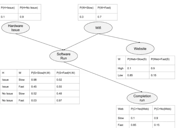
15 Figure 3.1 illustrates a simple example of Bayesian Network which depicts the proba-bility of the software run to complete, denoted byC. This is only dependent on whether the software is run at a high speed or low speed, denoted by S. The speed of the soft-ware is further dependent on whether there is a hardsoft-ware issue, represented by H, or if the WiFi speed is slow, represented by W. Also, there is high chance that if the wifi is slow, another website which is rendering some content also might be affected, denoted by W eb.

The joint probability distribution of all variables can be calculated as follows:

P(H, W, S, W eb, C) =P(H).P(W|H).P(S|H, W).P(W eb|H, W, S, C)

.P(C|H, W, S, W eb)

(3.3)

The total number of parameters required to compute this is 25 −1 = 31. However, based on this structure, we can observe some of the properties of Bayesian Network. H

and W do not depend on any other variables. However, whenS is given, they both fall in each other’s markov blanket and are conditionally dependent. Also, given a value for W, S and W are conditionally independent as they are outside markov blanket of each other. Similarly, C is independent of all other variables given S. Because of such properties, Bayesian Network provides a compact factorization of the equation 3.3 as follows:

P(H, W, S, W eb, C) =P(H).P(W).P(S|H, W).P(W eb|W).P(C|S) (3.4) Now, we can observe from the equation 3.4 that we need 1 parameter each forP(H) and

P(W), 2 parameters each forP(W eb|W) andP(C|S) and 4 parameters forP(S|H, W). Hence, the BN form reduces the number of the model parameters, which belong to a multinomial distribution in this case, from 31 to 10 (1+1+2+2+4) parameters. This reduction not only makes the learning computationally faster but it also makes the inference efficient by being robust to bias-variance trade-off.

Compared to learning the parameters of Bayesian Network, structure learning is a lot more difficult task. Learning a good topology of the Bayesian Network might require some prior information such as known causal relationships between attributes or other expert knowledge. With no prior knowledge, learning the best DAG structure is considered to be an NP-Complete [12] problem because the number of DAG structures

(26)

Figure 3.1: Illustration of software run completion using Bayesian Network

possible is exponential in terms of the number of random variables. Table 3.1 mentions the four scenarios for bayesian learning. Except for the first case, all other cases are computationally intractable [5]. For the second case, one can use EM to find a locally optimal maximum-likelihood estimate of the parameters. Third and fourth case requires searching through a model space in a greedy fashion which we will not be focusing on.

Case BN structure Observability Proposed learning method 1 Known Full Maximum-likelihood estimation 2 Known Partial EM (or gradient ascent), MCMC 3 Unknown Full Search through model space 4 Unknown Partial EM + search through model space

(27)

17

3.1.2 Autoencoder

Ian Goodfellow et al.[39] explains Deep Learning as”a subset of Machine Learning that achieves great power and flexibility by learning to represent the world as nested hierarchy of concepts, with each concept defined in relation to simpler concepts, and more abstract representations computed in terms of less abstract ones”. Deep learning techniques[57] learn the mapping of input space to some output space incrementally through its hidden layer architecture, defining low-level features (such as words in text, peripheral edges of an object in image) and then higher level features (such as sentences in text, specific entities in the image). Each hidden unit of a trained deep learning network represents one aspect of the whole and together they help represent the mapping from input space to final output space.

One of the deep learning networks used for the task of representation learning in an unsupervised manner is Autoencoders [53]. Autoencoders are the deep learning models which aim to understand the representation of the data by trying to reconstruct it. Figure 3.2 shows the simplest auto-encoder which has a multi-layer perceptron (MLP) - like structure with one hidden layer. The difference between an MLP and an autoencoder is that the output layer in the autoencoder has the same cardinality of its input layer whilst the cardinality of the output layer in an MLP is the number of classes the perceptron should be capable of classifying. The motivation for this architecture is that hidden layer represents latent features [4] which, in other words, are the representation of the input in smaller latent space. Hence, an autoencoder plays an important role in dimensionality reduction: after the training phase, the output layer is usually thrown away and the encoder network is used to build a new dataset of samples with lower dimensions.

Formal Definition

Formally, for a kth input vector xk, w1 and b1 represent the weights and bias of

en-coder networkE, andw2 and b2 represent the weights and bias of the decoder network D. A simple encoder could be represented as a network such that D(E(x)) =x. En-coder network E learns a stochastic mapping from input vector x to hidden vector

(28)

h as pencoder(h|x). Similarly, decoder network’s task is to learn the reverse

stochas-tic mapping as pdecoder(˜x|h) where ˜x represents generated input. Just like any deep

learning network, autoencoders are also trained using gradient descent technique where gradients are getting updated using backpropagation. The feed-forward computation in autoencoder can be mathematically written as follows:

h1 =a(w1x+b1) h2=a(w2h1+b2) . . . ˜ x=a(wnhn−1+bn)

where ais an activation function. The loss function for an autoencoder can be defined as follows: L(x, D(E(x)) = 1 2 X k ( ˜xk−xk)2 (3.5)

where, hidden layer h for an autoencoder with single hidden layer (as shown in figure 3.2) is computed as

E(x) =h=a(xk.w1+b1) (3.6)

where arepresents some activation function, and output layer ˜xcan be generated as

D(h) = ˆx=a(h.w2+b2) (3.7)

Here, ˜xk is the kth generated input and xk is the kth real input and Lrepresents total

squared reconstruction error.

3.2 Addressing limitations

Bayesian Network is a suitable machine learning model in many applications for various reasons [64]. One, Bayesian Network can give good generalization error even with fewer

(29)

19

Figure 3.2: Autoencoder with one hidden layer illustrating its two components: encoder and decoder

data. Two, Bayesian Network work even when the data is missing [52] which makes it a popular model for data imputation or interpolation [43] [23] as it encodes all variables. Three, Bayesian Network is very powerful for it can also learn the best structure [44] to represent the conditional dependence among the features. This improves the explain-ability aspect of the model. Four, because it learns the dependence of variables on each other, it can also be used for causal inference urther helping in understanding the prob-lem domain better. In fact, one can compute consequences given a cause and vice versa. This is done by calculating the probability of distributions of child nodes given parent nodes and vice versa. Five, Bayesian Network can be quick in answering queries once the model learns the structure and parameters as it contains the conditional probability distribution for every feature per every possible combination of its parent features.

However, Bayesian Network has several limitations [18], especially in the domain of collective anomaly detection when the anomalies are subtly anomalous when considered individually. We divide these limitations into 4 categories and explain each category of limitation and how they can be overcome by autoencoders.

First, Bayesian Networks work best with discrete variables. However, most of the real world data is continuous or a combination of discrete and continuous variables. Many techniques have been developed to deal with continuous variables. One such type

(30)

is discretization of continuous variables into intervals [30] [47] (i.e. changing continu-ous data into multinomial data). However, discretization might lead to some loss of information and Bayesian Network might end up learning approximate characteristics of the true distribution model. This might make the Bayesian Network lose its sta-tistical capability to detect subtle anomalies. Another type of approach is using naive bayesian structure [66], and then learn the distribution in a non-parametric way. Some techniques deal with continuous variables directly by assuming a certain distribution for every node in the network [37] and then learning its parameters. Real world data is too complex and such probabilistic assumptions might not often be true leading to loosely learned probability distribution. These techniques do not learn the true char-acteristics of the data [15] because of various assumptions which might be significant in detecting anomalies especially if they are subtly anomalous. On the other hand, au-toencoder is a non-parametric deep learning model that doesn’t assume anything about the data and can directly work with continuous data. Hence, it ends up learning the true characteristics of the data with more confidence.

Second, in order for Bayesian Network to be effective, the data must have some structure in it in terms of features being well defined. However, most real world data is unstructured. Furthermore, Bayesian Network needs to be pre-fed with extracted meaningful features [51] [60]. On the other hand, autoencoder can directly work with raw unstructured data. For example, for detecting heart irregularities through its sound, one needs to compute features such as audio signal type, strength, duration of the sound, frequency, etc. to come up with a structure in order to use Bayesian Network whereas audio signals can be directly fed to an autoencoder which can learn the probability distribution of the sound. For unstructured data, learning latent variables becomes extremely important in order to learn a better approximation of the true distribution of the data. However, it is difficult to learn latent variables using Bayesian Networks. Even though there are many techniques [16] [54] which can make Bayesian Networks learn latent variables, one needs to specify information such as the number of hidden variables, cardinality of each hidden node, etc. Identifying all possible combination of random variables is exponential [26] and hence, providing an optimal number of variables is challenging. Autoencoders, on the other end automatically learn latent variables representing significant features in hidden layers. This is convenient when the

(31)

21 underlying anomalous process is only subtly anomalous and can only be distinguished in latent space. Also, Bayesian Networks are not effective in learning high dimensional unstructured data such as images, genomic data, etc. As the dimension increases, the efficacy of Bayesian Network in learning conditional dependence among features decreases. Several techniques that use Bayesian Network to work with images, audio, etc., require extraction of meaningful features [50]. On the other, Autoencoder can work with such high dimensional data as it learns significant features given a large number of features and then anomalies can be detected based only on the small set of significant latent features learned.

Third, the power of Bayesian Network depends heavily on the structure learned. However, defining and learning the structure which represents the true data is a difficult task [13]. In order to provide good priors to the network, expert knowledge [42] is needed for modeling Bayesian Network. For instance, initial order of variables that are needed to be learned, subjective probability of a given variable to be the parent of another variable [55] for the nodes keeping the order of nodes specified under consideration, etc. Such knowledge is hard to be specified by an expert. Even though there are techniques developed for obtaining such prior knowledge based on statistical property of the data, it still relies on approximate assumptions. Such assumptions might give away crucial information making it hard to identify slightly anomalous records. On the other hand, autoencoder doesn’t assume anything in prior and instead starts with a randomly initialized weights and other defined hyperparameters and then tries to fit the data to that structure by updating weights, learning the statistical distribution that closely matches with the true distribution. Also, Bayesian Networks fail to learn the cyclic dependency among variables (for example, A depends B and B depends on A) and hence, can not learn the correlation between variables or combination of variables. In order for Bayesian Networks to learn the conditional dependence among features, all features must obey local markov property [5]. In fact, the structure learning problem itself is an N-P Complete problem. Though some techniques exist to relax the time complexity, they either follow a greedy approach based on some heuristics [56] [63] or restrict the space of models. In both cases, it might miss the best structure possible and learn an approximate model with high bias. Autoencoders, being a variant of Artificial Neural Network (ANN) which acts as a universal approximator [38], can learn

(32)

any structure without any restrictions like the absence of cyclic dependency, etc. This enables autoencoder to capture all dependencies and correlations in the data which might then make the detection of subtle collective anomalies efficient.

Four, there are several issues in training a Bayesian Network. One such issue is that learning the structure and parameters together is an NP-Complete problem [12]. This is because the objective function of the Bayesian Network is not a convex function. Although techniques [34] have been developed to make the objective function convex, it makes too many assumptions and as a result, the final learned model could actually be worse compared to the one obtained without the convex function. On the other hand, the objective function of autoencoders is based on the squared reconstruction error which is convex (refer equation 3.5). Also, in order to achieve good accuracy, Bayesian Network must learn all conditional dependencies among all variables. This might increase the model’s complexity drastically. One can say, as the accuracy increases, complexity could also increase. However, in case of autoencoder, one can fix the model’s complexity by various hyper-parameters like activation functions, number of hidden layers, number of hidden units in each layer, etc. And using gradient descent, it learns the best weights to fit the probability distribution and achieve desirable accuracy. From the qualitative perspective, one cannot justify how close the learned model is from true distribution because during the training process of Bayesian Network, the directions of dependence among variables might change multiple times and stop at a sub-optimal model. It can not be predicted if continuing the training process to next step gives a better model or worse. On the other hand, autoencoder’s training process involves finding a good local minima in a convex objective function using gradient descent and hence gives an idea of how far the given model is from the true model based on how soon the training process is halted.

There are many other limitations of Bayesian Network such as a Bayesian Network cannot be applied in an online setting. Generally, a block of data is given to the learning algorithm to learn the structure and its parameters. On the other hand, autoencoder being a deep learning network can be trained by providing one sample at a time using stochastic gradient descent with batch size being 1 and hence, can be used in an online setting. However, we will not be focussing on such limitations in this thesis.

(33)

Chapter 4

Proposed Solution

We employ a deep autoencoder network to learn the probability distribution of the data. More specifically, we use autoencoder to learn the hidden significant features in the normal data records under the H0. Using these hidden features, autoencoder

then reconstructs the input and provides reconstruction error for that particular input. We then convert these reconstruction errors into empirical p-value ranges and then run FGSS on them to get a subset S such that F(S) is maximum.

4.1 Property of reconstruction error

An autoencoder learns the significant features hidden in the latent space and recon-structs the input from those features with some errors. These reconstruction errors are independent and follow a normal distribution even though attributes are correlated. For one dimensional input, the magnitude of the reconstruction error tells how anoma-lous that input is. For multivariate input, one way to find out the anomaanoma-lousness of the input instance is the summation of reconstruction errors across all attributes for that input. However, we focus on individual attribute’s reconstruction error because our approach not only detects anomalous records but also provides information of the attributes whose reconstruction errors are unexpectedly high under H0.

First, we split the dataset containing only normal records into two sets, Datamodel

and Dataexp. We train the autoencoder on Datamodel to learn the probability

dis-tribution of the normal process that generated those records. Then, we generate the

(34)

reconstruction errors by feeding theDataexp to autoencoder. Let xij and ˜xij represent

the jth attribute of iith record for the original input xi ∈ Dataexp and reconstructed

input ˜xi respectively, wherej ∈[1, m] form attributes, reconstruction vector ri can be

represented as follows: ri=< ri1, ri2, ..., rij, ..., rim>= (xi−x˜i)2 (4.1) where, xi=< xi1, xi2, ..., xij, ..., xim> (4.2) ˜ xi=<x˜i1,x˜i2, ...,x˜ij, ...,x˜im> (4.3)

Here, rij indicates how likely is it to observe an attribute value for attribute j for

given recordxi. Higher the reconstruction errorrij, the more anomalous that attribute

value is for the record.

4.2 p-value ranges

While performing the hypothesis test in statistics, the p-value helps to determine the significance of the results. A p-value is a measure of the evidence against the null hy-pothesis. Lower p-value (typically≤0.05) indicates a stronger evidence against the null hypothesis, hence we reject the null hypothesis and accept the alternative hypothesis.

In the case of anomaly detection, a null hypothesis states that there are no anomalies present in the data and an alternative hypothesis states that the data contains anoma-lies. Typically, a lesserp-value for an instance indicates that the instance is an anomaly. For example, in Bayesian network [45], lesser p-value indicates lesser likelihood of that data instance under H0. However, in autoencoder, anomalous data instances tend to

have higher reconstruction error under H0. Thus, we define p-value metric such that

higher reconstruction errors correspond to lower p-values.

In order to compute the p-value, we first split the data containing no anomalies into Datamodel and Dataexp, train the autoencoder on Datamodel and calculate the

reconstruction errors onDataexp. These reconstruction errors represent the distribution

of the errors of each attribute underH0, represented by rij. Now, we take the test data

(35)

25 trained autoencoder underH0. Letrtij represent the reconstruction error ofjthattribute

of ith test record.

Traditionally, an empiricalp-value forjthattribute ofithtest record can be computed as pij =p(rtij) = 1 n Ntrain X k=1 I(rkj ≥rtij) (4.4)

where Ntrain denotes the total number of samples in Dataexp. One can note that

at-tributes which are anomalous will have lowerpij because of corresponding reconstruction

error rt_ij being larger. Apart from the test records having some true distribution, the reconstruction error rj of an attribute j also has some distribution of reconstruction

errors under H0. Since we know thatDataexp contains no anomalies in it, an empirical

cumulative distribution function can be calculated using equation 4.4. If Datatest has

no anomalies present in it, then r_ijt is from the same distribution as rij. In this case,

pij asymptotically follows a uniform distribution(0,1) for each j ∈ [1, m]. If Datatest

has few records which are slightly anomalous, then pij will not follow uniform

distri-bution(0,1) under H0. Similarly, the attribute which has slightly anomalous values for

some records are also not distributed as Uniform(0,1). This helps in getting insights about the attribute values which are slightly anomalous under H0.

McFowland et al. [45] suggested to use empiricalp-value ranges instead ofp-values to avoid the bias towards largerp-values when there is a chance of having tied likelihood values in the case of Bayesian networks, in our case, tied reconstruction error values. For example, consider a column j with all identical values. It will result inpij = 1 for each

record hence making it significant at some α. However, having all rt

ij with identical

values and similar to rij should not result in significant p-values. The occurrence of

this scenario is really low when the attributes are continuous. However, for discrete attributes (for eg. xij=0 for some xi), the autoencoder might reconstruct the exact

same value for that attribute, xt_ij resulting in identical p values. This leads to ties in reconstruction errors. Since most of the dataset might contain a mixture of continuous and discrete attributes, it is safer to use empirical p-value ranges compared top-values. To computep-value range for the reconstruction error ofjth _{attribute of} _ith _record,

(36)

we compute two terms Nbeat(rijt) = Ntrain X k=1 I(rt_ij < rkj) (4.5) Ntie(rijt) = Ntrain X k=1 I(rt_ij =rkj) (4.6)

Then, p-value range is a range bounded by two terms pmin and pmax i.e. [pmin(pij),

pmax(pij)] where, pmin(pij) = Nbeat(rijt) Ntrain+ 1 (4.7) pmax(pij) = Nbeat(rijt) +Ntie(rijt) + 1 Ntrain+ 1 (4.8)

Once we have empirical p-value ranges for each rt

ij, we can draw an empirical p-value

from this range and if DatatestandDataexp were from same distribution i.e. no

anoma-lies were present in Datatest, then the drawn empiricalp-values will be asymptotically

distributed as Uniform(0,1). With reference to the example of identical column values mentioned before, this approach would lead to Nbeat(rtij) = 0 andNtie(rtij) = 1. Hence,

this will result into an empiricalp-value range of (0,1), and randomly drawing ap-value from this range would result into Uniform(0,1) which verifies our intuition.

4.3 Testing Hypothesis

To carry out statistical hypothesis testing, we need to find a significance level α which is the probability of rejecting the null hypothesis when it is true. Typically, to detect whether a uni-variate data point is drawn from a given distribution, we first compute the p-value of that data point under the null hypothesis that the data point belongs to the given distribution. Then, at a particular significance level α, we reject the null hypothesis if p-value < α or p-value > 1−α. We define the significance of a given

p-value as

psig =I(p < α or p >1−α) (4.9)

In our approach, in order to determine whether a given subset is generated from an anomalous process, we first calculatep-value range for that subset. Then, we determine

(37)

27 the proportion of p-value range significant at α. In other words, the probability of a value drawn from [pmin(pij),pmax(pij)] is< α or>(1−α). In case of an autoencoder,

anomalous records or attributes tend to have higher reconstruction error underH0

lead-ing to lowerp-values. In other words, for the anomalous set of records, attributes which are anomalous have their corresponding pij < α. Hence, we determine the significance

of th jth attribute of ith record as follows:

psig(pij) =          0 ifpmin(pij)> α 1 ifpmax(pij)< α α−pmin(pij)

pmax(pij)−pmin(pij) otherwise

Then, significance of the subset S = RS ×AS can be determined by adding all the significance values in the subset as follows:

psig(S) = X i∈RS X j∈AS psig(pij) (4.10)

If we were considering a uni-variate data point such as psig(pij), we reject H0 if psig(pij)< α. However, in order to carry out hypothesis testing over the entire subset

S, we first compute the expected count of psig(pij)∈psig(S) significant at α as

pexp(S) =α×NS , where NS= X i∈RS X j∈AS 1 (4.11)

Informally, psig(S) denotes the observed number of p-value ranges in a subset S that

are significant at α. Each p-value range is determined by the proportion of the range significant at α. On the other hand, pexp(S) denotes the expected number of p-value

ranges in a subsetS that should be significant atα. Based on these two terms, we reject null hypothesis H0, if psig(S)> pexp(S), otherwise we assume that the subset contains

normal records.

4.4 Metric to determine atypicality of subets

If the autoencoder is perfectly trained ( i.e. it has learned the true typical characteristics of the normal records), it would be able to reconstruct the records with 0 reconstruc-tion error. However, for the anomalous records, the attributes which diverge more from

(38)

normal behavior tend to have higher reconstruction errors. We can note that the atypi-cality of the attribute value is measured by how far it’s reconstruction error is from the true expected value i.e. 0. Similarly, in order to determine the atypicality of the subset, we employ a non-parametric scan statistic called as the Berk Jones (BJ) statistic [6]. The BJ statistic for a given S gives us a score which indicates the divergence of the subset from the normal behavior. This divergence depends on the number of significant

p-value ranges in the subsetS. Formally, we employ the BJ statistic for a given S as follows:

τS = ΦBJ(psig(S), NS, α) =NS×K(

psig

NS

, α) (4.12)

whereK measures the Kullback-Liebler divergence between the observed proportion of significant p-values at α i.e. psig_NS and expected proportion ofp-values i.e. α.

Once we compute all the candidate subsets, the algorithm should calculateτS ∀ S,

and then returns the most anomalous subset S∗ such that τS∗ is maximum. However, computing all possible candidate subsets is exponential in N, and is infeasible for even moderately sized datasets.

(39)

29

Algorithm 1Deep FGSS

1. Given Training datasetDtrain, Testing datasetDtest

2. SplitDtrain intoDatamodel and Dataexp

3. Train Autoencoder onDmodel

4. Compute reconstruction error matrixEexp ={rij}

5. Compute reconstruction error matrixEtest ={rijt}

6. Computep-value matrixP ={pij}

7. For eachRi, form search group SGi={Rj}

8. For each SGg where g ∈ (1, G) and G denotes total

number of search groups

(a) Repeat for β number of iterations

i. InitializeA ←random set of {Aj}

ii. Repeat until convergence: A. SetR= max_R0F(R 0 ×A) B. SetA= max_A0F(R×A 0 ) iii. SetSg =R∗×A∗ 9. OutputS∗= maxSgF(Sg)

4.5 Efficient Search Technique

In order to resolve the issue of exponential time complexity of computing all possible subsets, most of the anomalous pattern detection techniques put some restrictions in the search space or follow a greedy approach to find the best set of subsets. Hence, these techniques might miss the most anomalous subset present in the dataset. Also, these techniques do not scale well with the size of the dataset, making it infeasible for larger datasets.

(40)

Daniel B. Neill [48] devised LTSS property which enables searching only N of the 2N possible subsets of records and still provides us the guarantee of finding the most anomalous subset. The LTSS property states that If we have a scoring function F(S)

to maximize over all subsets of records, and a ranking function G(Ri) which assigns a

rank Γi ∈ (1, N) to Ri, the subset S∗ with the maximum score F(S∗) consists of the

top-k ranked records. In our case we have

F(S) =τS (4.13)

G(Ri) =

X

j∈(1,M)

psig(pij) (4.14)

The intuition behind the above ranking function is that the anomalous records tend to have larger reconstruction error rij for some of the attributes, and inturn a larger

reconstruction errorri for the entire record. This results in a larger number of significant

p-value ranges at levelαfor that record. This leads to a higherG(Ri) value for the more

anomalous record than the record which is slightly lesser anomalous. The records which are not generated by any anomalous process will have very fewer or no significant p -value ranges leading to lowerG(Ri) values. If we sort all the records in descending order

based on their corresponding G(Ri) values, we can form the subset S(k) =R(k)×Ain a

smarter way by including only the set of top-kranked recordsR(k)={Ri} ∀Γi ∈(1, k)

such thatF(S(k)₎_{> F}₍_S(k+1)_{). This happens when the (}_k_{+ 1)}th_{ranked record has zero}

or very less number of significant p-value ranges and is likely a normal record. Hence, intuitively all the subsequently lower ranked records with Γi ≥k+ 1 are also likely to

be generated by the normal process.

This way we can find the most anomalous subset of records given all the attributes. In order to identify the most anomalous subset of columns for a given set of records, we can perform the same optimization step for columns. For the given set of records, we can rank all the columns according to their corresponding values of G(Aj) and incorporate

only the top-kattributes in the subsetS(k

0 )₌_R_×_A(k0)_where_A(k0) ₌_{_A j} ∀Γj ∈(1, k) such thatF(S(k 0 ))> F(S(k 0

+1)_{). Note that, here Γ}

j indicates the rank of the attribute

instead of record.

Formally, we define the above two optimization [36] steps for someα, total number of records N and total number of columns M as follows:

(41)

31

Step 1: For the set of columnsAj forj∈(1, M), rank all the recordsRi fori∈(1, N)

using the ranking function as

G(Ri) =

X

j∈(1,M)

psig(pij) (4.15)

and then find R(k)={Rl: Γl ∈(1, k)} such thatF(R(k)×A)> F(R(k+1)×A)

Step 2: For the set of rows Ri for i∈ (1, N), rank all the columns Aj for j ∈ (1, M)

using the ranking function as

G(Aj) =

X

i∈(1,N)

psig(pij) (4.16)

and then find A(k) ={Al : Γl∈(1, k)}such that F(R×A(k))> F(R×A(k+1))

Once we find R(k) in the Step 1, we set R=R(k). Step 2 gives A(k) for the current set of records R. We then set A=A(k)_{. We repeat the above two steps alternatively and}

at the end of every iteration we keep getting a better set of records and columns which maximizesF(S). We stop this alternative process until we find the most optimal subset

S∗ =R∗×A∗ such thatF(S∗) is maximum. Intuitively, we treat the entire data as the subset and keep shortening the subset by removing a set of records and columns. The criteria for the removal is that the difference between the observed number and expected number of significantp-value ranges should increase. This repeats until it converges i.e. when the difference is maximum. At this point, we obtain the most anomalous subset in the entire dataset. Note that we always start the alternating optimization process with a random set of columns or records. Hence, we repeat this convergence process for different random initialization and return the subset with a maximum score among all such iterations.

The underlying assumption is that all normal records are generated by a single back-ground process and we learn the characteristics of this process using autoencoder under

H0. Also, there is a separate anomalous process that generates anomalous records whose

characteristics are different compared to the normal process. We can take advantage of such a disparity by inducing similarity constraint to group similar records. We then run the above optimization process within each group. This will return not only the most optimal subset but also ensures that all the detected records have self-similar charac-teristics. Another advantage of enforcing a similarity constraint is that in the presence

(42)

of different types of anomalies, it will ensure that the detected subset contains all the records that belong to a single anomaly type. Different types of anomalies are generated by their corresponding anomalous processes which differ slightly from each other. To compute the similarity between two records, we can use metrics like Euclidean distance, Correlation-coefficient, Cosine similarity, etc. Formally, a search group for a recordRiof

radiusrcan be defined as{Rj :d(Ri, Rj)≤r}wheredmeasures the similarity between

two data records. We can choose r depending on how strictly we want to enforce the similarity constraint. Also, one should be careful in choosing the metric as it depends on the input type. For instance, choosing Euclidean distance as the distance metric for images might not be suitable. A similarity metric should give a high value while comparing two normal records and a low value if we compare a normal record with an anomalous record.

4.6 DeepFGSS Algorithm

DeepFGSS algorithm is an extension of the original FGSS algorithm [45] developed by McFowland et al. which uses deep networks like autoencoders to enable FGSS to work with high dimensional unstructured data with both discrete and continuous attributes. Note that DeepFGSS works not only with autoencoder but any deep neural network architecture for learning the probability distribution under the null hypothesis.

We illustrate the main steps of DeepFGSS in algorithm 1. We first split the training data that contains no anomalies into two parts: Datamodel and Dataexp and train

autoencoder onDatamodel to learn the probability distribution of normal records under

the null hypothesisH0 that no anomalies are present. We then calculate reconstruction

error of Dataexp as Eexp which represents the expected distribution of reconstruction

errors of data under H0. We also calculate reconstruction errors of theDatatestasEtest

and then, computep-value ranges for the reconstruction errors of each record’s attribute value r_ijt ∈Etest by comparing it with the reconstruction errorsrij ∈Eexp ∀i∈(1, N)

of the same column j. We then randomly draw a p-value pij ∈ Uniform[pmin(pij),

pmax(pij)] for all the attributes for each record. Optionally, we can enforce similarity

constraints by forming search groups for eachRi inDatatest using some distance metric

(43)

33 search group and identify the most anomalous subset in that search group as Sg. The

algorithm then returns the subset Sg with maximum BJ statistic scoreF(Sg) as S∗.

Note that, unlike FGSS, there is an additional requirement in DeepFGSS to store the distribution of the normal dataEexp along with the trained model which represents

the expected probability distribution of the normal data. Autoencoder maps the raw input space to the probability distribution space of reconstruction errors.

There are various parameters that can be manually tuned in DeepFGSS. In order to choose the significance level α, one can consider all the unique reconstruction error values in the test dataset within some αmax and run the optimization steps for each of

the unique α ≤ αmax. The value of the αmax can be set depending on the disparity

between anomalous and normal records. Anomalies which are easily detectable lie on the extreme corners when you plot the distribution of the normal records. However, anomalies which are slightly anomalous, when considered individually, tend to share many characteristics with the normal records and hence do not necessarily lie on the extreme ends of the distribution. Also, one can choose any distance metricddepending on the data and radius r depending on how small/strict the neighborhood should be. Apart from these, if we have some prior expert knowledge of the data, we can add tweaks such as the minimum or the maximum number of records a neighborhood can have. We can also choose other non-parametric scan statistics such as the Higher Criticism (HC) [25] statistics which can determine the similarity between two subsets. Along with these parameters, the deep learning model itself can be treated as a parameter where one can choose models such as Bidirectional Generative Adversarial Network [24] , Long Short Term Memory [7] for time series data, etc. We do not employ any other model in this thesis but the similar idea can be extended to other deep learning models and use FGSS on top of it.

4.7 Computational Complexity

The most critical challenge in anomalous pattern detection is the infeasibility of eval-uating all the possible subsets of the dataset. Even for a moderately sized dataset consisting of N records and M attributes, there are a total number of 2N×2M possible subsets.

(44)

FGSS takes advantage of LTSS property to reduce the problem of evaluating all subsets from O(2N ×2M) to O(N). To compute ranks for each record, we need to sum over the psig of all the attributes in O(M) complexity for each record leading

to O(N M) for all records. After computing the ranks for all the records, sorting them takesO(NlogN). The worse case time complexity for evaluating top-kranked subsets is

O(N). Similarly, for ranking each column, computingpsig for all records takesO(M N)

and sorting them takesO(MlogM). Hence, evaluating top-kranked subsets of columns takes the worst case time complexity ofO(M). Each single optimization run comprises of maximizing over both records and columns that takes time complexity of

O(N M) +O(NlogN) +O(N) +O(M N) +O(MlogM) +O(M) =

O(N M+NlogN +MlogM)

(4.17)

Considering γ is the average number of times the optimization ran before converging for each β number of iterations, and u is number of unique alpha values ≤αmax, the

total time complexity becomes

u×β×γ×O(N M+NlogN +MlogM) =O(uβγ(N M+NlogN +MlogM)) (4.18) On enforcing similarity constraints, FGSS runs within each neighborhood. The max-imum number of neighborhoods possible is N with k being the maximum number of records a neighborhood can be comprised of. In case of constrained FGSS, total time complexity across all neighborhood becomes

O(uβγN(kM +klogk+MlogM)) (4.19)

Note that the above time complexity is still less thanO(2N×2M). Also, one can enforce stricter constraints on the number of neighborhoods, minimum/maximum neighborhood size (k) and number of unique alpha values (u) to improve the running time with a reduced chance of finding the most optimal subset.

(45)

Chapter 5

Evaluations

In this section, we explain the performance of DeepFGSS on two datasets: network intrusion and handwritten digits. We evaluate the performance in two ways. One, we measure the efficiency of how well DeepFGSS can distinguish between datasets contain-ing and not containcontain-ing anomalies. We plot power curve and ROC curve for evaluatcontain-ing this measure. The other performance metric determines how well DeepFGSS can detect anomalies in the dataset. We plot jaccard curve and precision-recall curve for determin-ing the detection accuracy. We compute these metrics for varydetermin-ing dataset sizes, namely 100, 250, 500, 750 and 1000 with varying proportion of anomalies, namely 0%, 3%, 6%, 9%, 12% and 15%.

5.1 Experiments

5.1.1 Power curve

Power of an algorithm is defined as the probability of rejecting the null hypothesis when it is false. In our case, null hypothesis H0 represents no anomalies are present in the

dataset and alternative hypothesis H1 represents the dataset contains some anomalies.

Mathematically, power can be defined as follows:

power =p(rejectH0|H1 is true) (5.1)

Power of DeepFGSS depends on three primary factors: significance criterion, size of the dataset and the proportion of anomalous records. We study the power of DeepFGSS

(46)

at a significance criterion, αp = 0.05, for dataset size N varying as 100, 250, 500, 750

and 1000 with proportion of anomalies prop increasing as 0%, 3%, 6%, 9%, 12% and 15%. To calculate the power at a givenN andprop, we first randomly draw 100 datasets

Dnormalconsisting ofN number of records with no anomalies in it and 10 datasetsDtest

of N number of records withprop% anomalies in it and calculate the dataset score for each of them. We define the dataset score as the score of the most anomalous subset found in that dataset i.e.

τ_Di =τ_S∗_⊆_Di (5.2)

where S∗ is the most anomalous subset in ith drawn dataset Di. We then compute the power of DeepFGSS for Dtest at a given dataset size N and proportion of anomalies

prop as follows: O_beatsi = 100 X j=1 I(τ_Di test > τDjnormal) Ebeats= 100×(1−αp) power(Dtest) = P10 i=1I(Oibeats> Ebeats) 10

Here, Obeats is the observed number of times the score of the anomalous dataset is

greater than scores of normal datasets drawn whereas Ebeats is the expected number

of times the score of the anomalous dataset must be greater than the scores of normal datasets drawn.

Informally, power of the DeepFGSS tells what should be the minimum proportion of anomalies in order for the algorithm to perform well for a given dataset size at a given significance criterion. For example, a power of 0.7 means that 7/10 times DeepFGSS is able to detect anomalous subsets (which makes the score of the dataset higher) in a given sized dataset and given proportion of anomalies.

5.1.2 ROC curve

In this experiment, we treat the task of distinguishing normal and anomalous datasets as a binary classification problem and plot Receiver Operating Characteristic (ROC)