A robust optimization approach to statistical estimation problems by Apostolos G. Fertis.

A Robust Optimization Approach to Statistical

Estimation Problems

by

Apostolos G. Fertis

Submitted to the Department of Electrical Engineering and Computer

Science

in partial fulfillment of the requirements for the degree of

Doctor of Philosophy in Electrical Engineering and Computer Science

at the

MASSACHUSETTS INSTITUTE OF TECHNOLOGY

June 2009

@ Massachusetts Institute of Technology 2009. All rights reserved.

ARCHIVES

A uth or ...

Department of Electrical Engineering and Computer Science

May 19, 2009

Certified by ...

-

'tDimitris

J. Bertsimas

Boeing Professor of Operations Research

Sloan School of Management

Thesis Supervisor

Accepted by...

Terry P. Orlando

Chairman, Department Committee on Graduate Students

MASSACHUSETTS INSTITUTE OF TECHNOLOGY

AUG

07

2009

LIBRARIES

A Robust Optimization Approach to Statistical Estimation

Problems

by

Apostolos G. Fertis

Submitted to the Department of Electrical Engineering and Computer Science on May 19, 2009, in partial fulfillment of the

requirements for the degree of

Doctor of Philosophy in Electrical Engineering and Computer Science

Abstract

There have long been intuitive connections between robustness and regularization in statis-tical estimation, for example, in lasso and support vector machines. In the first part of the thesis, we formalize these connections using robust optimization. Specifically

(a) We show that in classical regression, regularized estimators like lasso can be derived by applying robust optimization to the classical least squares problem. We discover the explicit connection between the size and the structure of the uncertainty set used in the robust estimator, with the coefficient and the kind of norm used in regularization. We compare the out-of-sample performance of the nominal and the robust estimators in computer generated and real data.

(b) We prove that the support vector machines estimator is also a robust estimator of some nominal classification estimator (this last fact was also observed independently and si-multaneously by Xu, Caramanis, and Mannor [52]). We generalize the support vector machines estimator by considering several sizes and structures for the uncertainty sets, and proving that the respective max-min optimization problems can be expressed as regularization problems.

In the second part of the thesis, we turn our attention to constructing robust maximum likelihood estimators. Specifically

(a) We define robust estimators for the logistic regression model, taking into consideration uncertainty in the independent variables, in the response variable, and in both. We consider several structures for the uncertainty sets, and prove that, in all cases, they lead to convex optimization problems. We provide efficient algorithms to compute the estimates in all cases. We report on the out-of-sample performance of the robust, as well as the nominal estimators in both computer generated and real data sets, and conclude that the robust estimators achieve a higher success rate.

(b) We develop a robust maximum likelihood estimator for the multivariate normal distri-bution by considering uncertainty sets for the data used to produce it. We develop an efficient first order gradient descent method to compute the estimate and compare the

efficiency of the robust estimate to the respective nominal one in computer generated data.

Thesis Supervisor: Dimitris J. Bertsimas Title: Boeing Professor of Operations Research Sloan School of Management

Acknowledgements

I would like to express my gratitude for my supervisor Professor Dimitris Bertsimas for in-spiring me throughout my PhD research. He has been very helpful in identifying challenging problems, providing his insight and encouraging my endeavors, even in difficult situations. Furthermore, I would like to thank Professors Pablo Parrilo, Georgia Perakis and John Tsit-siklis, who, as members of my PhD committee, aided me with experienced comments and thoughtful observations. I would also like to thank Dr. Omid Nohadani for supporting me with his cooperation and advice, and for providing his very wise views in our long conver-sations. Finally, I am very grateful to my family, my father George, my mother Lori, and my sister Andriani, as well as my friends, for believing faithfully in my dreams and always providing me with invaluable support to overcome any obstacle I met.

Contents

1 Introduction

₁₃

1.1 Robust Optimization in Statistical

Estimation Problems .. ... . . . 14

1.2 Contributions of the Thesis . ... 15

2 Equivalence of Robust Regression and Regularized Regression

17

2.2 Robust Regression .. . . ... ... . . . . .. .... ... . 18

2.3 Support Vector Machines for Regression ... ... . . 23

2.4 Experimental Results ... . . . . ... . 26

2.5 Conclusions ... ... ... ... .... . 31

3 Support Vector Machines as Robust Estimators 33 3.1 Introduction . . . . ... . . ... .. ... . . . 33

3.2 Robust Properties of Support Vector Machines . ... . ... .. 34

3.3 Experimental Results ... . . 39

3.4 Conclusions . . . . .. .. ... . . . . . 40

4 Robust Logistic Regression 43 4.1 Logistic Regression ... . . 43

4.2 Robust logistic regression under independent variables uncertainty ... 44

4.3 _{Robust logistic regression under response variable uncertainty . ... 47}

4.4 Globally robust logistic regression ... ... 49

4.5 Experimental Results .. . . . . . ... ... . . 55

4.5.1 Artificial Data Sets . . . . . ... ... .. .. . . . 55

4.5.2 Real Data Sets ... ... . ... ... . 56

5 Robust Maximum Likelihood In Normally Distributed Data

5.1 Introduction . . . . 5.2 M ethod . . . .

5.3 Experiments . . . . ...

5.3.1 Worst-Case and Average Probability Density . 5.3.2 Distance From the Nominal Estimator . . . . 5.3.3 Comparison of the Error Distributions . . . . 5.4 Conclusions . . . ...

A Algebraic Propositions

A.1 Properties of function f(x,p) ... A.2 Propositions on matrix norms ...

B Robust Logistic Regression Algorithms

B.1 Robust logistic regression under independent variables algorithm .... ...

77

uncertainty solution

. .

. . . . 77

B.2 Robust logistic regression under response variable uncertainty solution algorithm 78

B.3 Globally robust logistic regression solution algorithm . ...

79

C The partial derivatives of

Z

(0, 0o)

and

Z

(/3,

o)

81

... . . . . . 6 1 ... . . . . 6 1 ... . . . . 68 . . . . 69 . . . . 70 . . . . 7 1 ... . . . . . 7 1 73 .. . . . 73 .. . . . 74

List of Figures

2-1 _{The average mean absolute error of the regression estimates according to p. . 28} 2-2 The average mean squared error of the regression estimates according to p. . 29 3-1 The average classification error of the classification estimates according to p. 40 4-1 Success rate of the robust logistic regression under independent variables

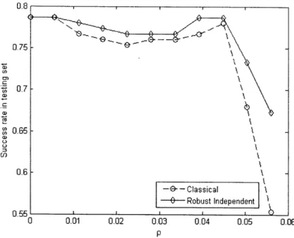
un-certainty estimate in the testing set... ... ... . . 56

4-2 Success rate of the robust logistic regression under response variable uncer-tainty estimate in the testing set. . ... ... 57

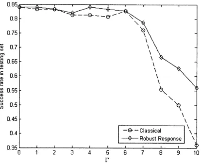
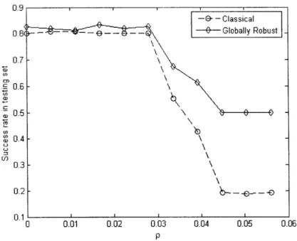
4-3 Success rate of the globally robust logistic regression estimate in the testing set (F = 1) . ... ... . ... ... ... ... . . 57

4-4 Success rate of the globally robust logistic regression estimate in the testing set (F = 2). ... .. . ... ... . . . 58

5-1 Worst-case (left) and average (right) value of 0, normal errors ... 69

5-2 Error in tp (left) and F (right), normal errors . ... 71

List of Tables

2.1 Sizes of real data sets for regression ... .... . 29 2.2 Mean absolute error in testing set for real data sets. * denotes the estimate

with the best performance. ... . ... .. 30 2.3 Mean squared error in testing set for real data sets. * denotes the estimate

with the best performance. . ... . ... .. 31 3.1 Sizes of real data sets for classification. ... .. 41 3.2 Classification error in testing set for real data sets. * denotes the estimate

with the best performance. ... . ... .. 41 4.1 Sizes of real data sets. . ... . . ... . 59 4.2 Success rate in testing set for real data sets. * denotes the estimate with the

Chapter 1

Introduction

Statistical estimation has a long and distinguished history. In the context of regression, the idea of least squares has been used extensively. More generally, the established paradigm is to use the maximum likelihood principles.

Researchers soon realized that data on which these estimators are based are subject to error. The origins of the errors can be multiple (measurement, reporting, even classification (a clinical trial can be classified as success while it can be indeed a failure)). In order to deal with errors several researchers have introduced regularization methods:

a) Regularized regression. Given a set of observations (yi, xi), yi E I, xi E Rm, i E {1, 2,..., n}, Tibshirani [49] defines the Least Absolute Shrinkage and Selection Operator (lasso) estimate as the optimal solution to the optimization problem

min ly - X0 - 3o112 + p1l3III1,

(1.1)

where

Yl xt 1

y = , X = 1 = entries, (1.2)

Yn Xn

and p > 0. Tibshirani [49] _{demonstrated using simulation results that the lasso estimate}

tends to have small support which yields more adaptive models and higher empirical success. Tikhonov and Arsenin proposed the ridge regression estimate, which is the

solution to

mmin Ily - X3 - olII + p1P3I| , (1.3)

see [50].

b) Support vector machines in classification problems, introduced by Vapnik et al. [10]. Given a set of data (y,x i), i E {1,2,...,n}, y E {-1,1}, x~ I Rm, the support vector machines estimate is the optimal solution to optimization problem

n

min II12+P2 P i

3,13o, i=1

s.t.

2 1 - yi(3'xi +/30),i

{1,2,...,n}

(1.4)

i > 0,i E {1,2,...,n},

where p > 0. Support vector machines classifiers have been very successful in experiments (see Scholkopf [43]). Note that Problem (1.4) has a regularization term

110112

Huber [30] considers any statistical estimator T to be a functional defined on the space of probability measures. An estimator is called robust, if functional T is continuous in a neighborhood around the true distribution of the data. Hampel defined the influence curve to quantify the robustness of statistical estimators [26]. However, they did not provide an algorithmic way to construct robust estimators.

1.1

Robust Optimization in Statistical

Estimation Problems

In this thesis, we use the paradigm of Robust Optimization to design estimators that are immune to data errors. Before describing the specific contributions of the thesis, let us give a brief overview of Robust Optimization.

Robust optimization has been increasingly used in mathematical programming as an effective way to immunize solutions against data uncertainty. If the data of a problem is not equal to its nominal value, the optimal solution calculated using the contaminated data might not be optimal or even feasible using the true values of the data. Robust optimization considers uncertainty sets for the data of the problem and aims to calculate solutions that

are immune to such uncertainty. In general, consider optimization problem

min f(x; d)

xEX

with decision variable x restricted in feasible set X and data d. The robust version of it, if we consider uncertainty set D for the errors Ad in the data, is

min max f(x; d + Ad).

xEX AdED

As we observe, the efficient solution of the nominal problem does not guarantee the efficient solution of the respective robust one.

There are many ways to define uncertainty sets. Soyster [47] considers uncertainty sets in linear optimization problems where each column of the data belongs to a convex set. Ben-Tal and Nemirovski [4], [5], _{[6], follow a less conservative approach by considering uncertain}

linear optimization problems with ellipsoidal uncertainty sets and computing robust coun-terparts, which constitute conic quadratic problems. Bertsimas and Sim [8], [9], consider an uncertainty set for linear or integer optimization problems where the number of coefficients in each constraint subject to error is bounded by some parameter adjusting the level of conservatism, and prove that this problem has an equivalent linear or integer optimization formulation, respectively.

The idea of using robust optimization to define estimators that tackle the uncertainty of the statistical data has already been explored. El Ghaoui and Lebret [20] have used robust optimization to deal with errors in the regression data. They define the robust total least squares problem, where the Frobenious norm of the matrix consisting of the independent variables and the response variable of the observations is bounded by some parameter, and prove that it can be formulated as a second order cone problem.

1.2

Contributions of the Thesis

In this thesis, we apply robust optimization principles to many classical statistical estimation problems to define the respective robust estimators, that deal with errors in the statistical data used to produce them. We study the properties of the estimators, as well as their connection with the uncertainty set used to define them. We develop efficient algorithms that compute the robust estimators, and test their prediction accuracy on computer generated as well as real data.

In the first part of the thesis, we formalize the connections between robustness and regularization in statistical estimation using robust optimization. Specifically

(a) We show that in classical regression, regularized estimators like lasso can be derived by

applying robust optimization to the classical least squares problem. We discover the

explicit connection between the size and the structure of the uncertainty set used in

the robust estimator, with the coefficient and the kind of norm used in regularization.

We compare the out-of-sample performance of the nominal and the robust estimators in

computer generated and real data.

(b) We prove that the support vector machines estimator is also a robust estimator of some

nominal classification estimator (this last fact was also observed independently and

si-multaneously by Xu, Caramanis, and Mannor

[52]).

We generalize the support vector

machines estimator by considering several sizes and structures for the uncertainty sets,

and proving that the respective max-min optimization problems can be expressed as

regularization problems.

In the second part of the thesis, we turn our attention to constructing robust maximum

likelihood estimators. Specifically

(a) We define robust estimators for the logistic regression model, taking into consideration

uncertainty in the independent variables, in the response variable, and in both. We

consider several structures for the uncertainty sets, and prove that, in all cases, they

lead to convex optimization problems. We provide efficient algorithms to compute the

estimates in all cases. We report on the out-of-sample performance of the robust, as well

as the nominal estimators in both computer generated and real data sets, and conclude

that the robust estimators achieve a higher success rate.

(b) We develop a robust maximum likelihood estimator for the multivariate normal

distri-bution by considering uncertainty sets for the data used to produce it. We develop an

efficient first order gradient descent method to compute the estimate and compare the

efficiency of the robust estimate to the respective nominal one in computer generated

data.

The structure of the thesis is the following. In Chapter 2, the connection between robust

regression and regularized regression is quantified and studied. In Chapter 3, the

Sup-port Vector Machines estimator is proved to be the robust estimator corresponding to some

nominal classification estimator, and its properties are investigated. In Chapter 4, robust

estimators for logistic regression are defined and calculated. In Chapter 5, a robust normal

distribution estimator is defined, and an efficient algorithm to calculate it is developed.

Chapter 2

Equivalence of Robust Regression and

Regularized Regression

2.1

Introduction

A way to improve the performance of the regression estimate is to impose a regularization term in the objective function of the optimization problem which defines it. Given a set of observations (yi, xi), y E I E m, i E {1,2,..., n}, Tibshirani [49] defines the Least

Absolute Shrinkage and Selection Operator (lasso) estimate as the optimal solution to the optimization problem min

1y

Tibshirani [49] demonstrated using simulation results that the lasso estimate tends to have small support which yields more adaptive models and higher empirical success. Candes and Plan [13] proved that if the coefficient vector 3 and the data matrix X follow certain probability distributions then, lasso nearly selects the best subset of variables with non-zero coefficients.

The connection between Robust Optimization and Regularization has been explored in

the past. El Ghaoui and Lebret prove that the minimization of the worst-case least squares

error can be formulated as a Tikhonov regularization procedure [20]. Golub et al proved that

Tikhonov' s regularization method can be expressed as a total least squares formulation,

where both the coefficient matrix and the right-hand side are known to reside in some sets.

In this chapter, we prove that regularization and robust optimization are essentially

equivalent, that is the application of the robust optimization paradigm in statistical

estima-tion leads to regularized soluestima-tions. We investigate the nature of the regularized soluestima-tions

as the uncertainty sets in robust optimization vary. We present empirical evidence that

demonstrates that the application of robust optimization in statistics, which is equivalent to

regularization, has an improved out-of-sample performance in both artificial and real data.

We further investigate the effectiveness of different uncertainty sets and their corresponding

regularizations. In summary, the key contribution of this section is that the strong empirical

performance of regularized solutions, which we also observe in this paper, can be explained by

the fact that the process of regularization immunizes the estimation from data uncertainty.

The structure of the chapter is as follows. In Section 2.2, we prove that the robust

regression estimate for uncertainty sets of various kinds of norms can be expressed as a

regularized regression problem, and we calculate the relation between the norms used to

define the uncertainty sets and the norms used in regularization, as well as their coefficients.

In Section 2.3, we prove that the optimization problem used to define the support vector

machines regression estimate is the robust counterpart of the e-insensitive regression estimate

problem. In Section 2.4, we report on the improved out-of-sample performance of the robust

and regularized estimates in comparison to the classical ones in the experiments we carried

out on artificial and real data.

2.2

Robust Regression

Given a set of data (yi, xi), y CE

R, xi E

IR

_,

_{i E {1, 2,}

_...

, n}, we consider the Robust LP

Regression optimization problem

min

max

Iy

-

(X + AX)/3 - /

ol p,

(2.3)

)3,0o AXEAf

where y, X, and 1 are defined in Eq. (2.2) and

K

is the uncertainty set for AX.

The uncertainty sets for AX are going to be defined by bounding various kinds of norms

of matrix AX. There exist several matrix norms (see Golub and Van Loan [24]). For

example, norm

I

* Iq,p for an n x m matrix A is defined by

I A9lq,p

sup

qp

>

1,

xERm,x$O jjXjjq

see Golub and Van Loan [24], p. 56.

Note that

IIA

lq,p

=

max

IIAxl p,

11Xllq=l

and that for some x* E

R

_IIX*Ilq

_1,

IIAIIq,p =IIA *llp,

see Golub and Van Loan [24], p. 56.

Moreover, we define the p-Frobenius norm which is also going to be used in defining

uncer-tainty sets for AX.

Definition 1. The p-Frobenius norm I* tJp-F of an n x m matrix A is

i=1 j=1

Observe that for p = 2, we obtain the usual Frobenius norm.

The following theorem computes a robust counterpart for the robust optimization Problem

(2.3) under the uncertainty sets

N' = {AX E R

I lAXllq,p < p},

(2.4)

and

N -2 =

{AX

c

It proves that the robust regression problems under these uncertainty sets can be expressed

as regression regularization problems.

Theorem 1.

(a)

min Ily

-

Xp -

/3oll0p +

P11

_1|q.

_(2.6)

(b) Under uncertainty set N2, Problem (2.3) is equivalent to problem

min

Il

- X3

-

00o111p

+

pll

d(p),

13,1o where .f1, '2 are defined in Eq.

(4.3).

Proof.

(2.4) and (2.5) respectively, and d(p) is defined in Eq.

(a) The proof utilizes Appendix A.2 that performs certain somewhat tedious vector calcu-lations. To prove the theorem, we shall first compute a bound for the objective function of the inner problem in Eq. (2.3) and then, calculate a AX that achieves this bound.

Using the norm properties, we have that

Ily - (X + AX)3

-

00ollP

=-

3ol

< Ily-X3- 3olp +

IlAXl3p.

From Golub and Van Loan [24], p. 56, we have that

IlX3llp

_

IlAXllq,p

11)-IIl

Thus, for IlAX llq,p < p,

and for any AX

cEM,

IlY

-

(X + AX)3

-

/3o111p

AXo

=

Ily

- Xp

3olI,

+

PII

_Pl1q.

We next construct a solution AXo E Nli that achieves bound (2.8). Let

Y - X _{- 001 [f(P, q)} ]T, |ly - X3 - ollp -pu[f(, q)] , if Y - X3 - 3ol 0, if y - X - 3ol = 0,

where f(x,p) E rn, x E R , p > 1, is defined in Eq. (A.1) in Appendix A.2, u E RI " is an arbitrary vector with

Ilullp

(2.7)

(2.8)

(2.9)

For y - Xf3 -

31

Ily

-

(X + AX)3 /3olIp

-- y

Ily - X3 - 3ol - AXo3P1

]To

P

([f(0,

q)]

_,

=

IIlI0q)

Note that when y - X3 - 3ol = 0, Ily - (X + AXo)f3 -

/

olll

/ol|p +

+/

as well.

Moreover, using Propositions 1 and 3 in Appendix A.2, we have that if y - X3 - /ol = 0,

IAXollq,p = Y - X3 -

/3l 1

If(/3,

q)

liy

/3ollIp

and if y - X3 -3 ₀1= O,

I|AXoII,, = pllullpll,

f(,

q)

Ild()

=

p.

Thus, AXoE . f.

Consequently, we conclude that

max Ily - (X + AX)

3

-

3o111p

= |ly - XO -

3o111p

+ PIIPl

q,

axEnr,

which proves the theorem.

(b) Following the same procedure, we conclude that

Ily

- (X

+ AX)

- ,3o111

ly

-

X3

-

/3olI,

+

IIAX0/3

.

From Golub and Van Loan [24], p. 56, we have that

lAX/1p

- IIAX ld(p),

11 1

d(p).

y - XO - o1

- Xp -/3ol + p-y -/3o [f ( , q )

|yv- Xp-

Using Proposition 2 in Appendix A.2, we conclude that

IIAX)31,

<

IIAXllp-F

1l01ld(p,

and thus, for any AX E N/2,

IIv

IY

Pll/lld(p)-Define AX0 _{as in Eq. (2.9) with q = d(p). Then,}

Ily

-

(X + AXo)3 -

00olll

= liy - X1 -

1ol1I,

+

PllPlld(p)-Furthermore, using Propositions 1 and 4 in Appendix A.2, we have that if y - XP3 -ol

#'

IIAXoIIPF -=

y -

*

f(03,

Iy

and if y - X3 - ol = 0,

IlAXollp-F

=

-

and consequently, AXo E NV. This allows us to state that

max Ily - (X + AX) -- 131I11 =

Iy

/3oill

AXEAr2

which proves the theorem. O

Theorem 1 states that protecting the regression estimate against errors in the independent variables data bounded according to certain matrix norms is achieved by regularizing the corresponding optimization problem. The structure of the uncertainty set determines the norm which is going to be considered in the regularized problem. The conservativeness of the estimate is affected by parameter p, which determines the size of the uncertainty set as well as the contribution of the norm of the coefficient vector to the objective function to be minimized in the robust counterpart.

2.3

Support Vector Machines for Regression

Consider the E-insensitive regression estimate which minimizes the E-insensitive loss function

n

mm max(0, yi - ,Txi -

30

The corresponding robust regression estimate, which immunizes against errors described by the uncertainty set A3 is

n

minm max max(0,

jyi

13oI

P,o AXEA 3 _i=1

where '/3 is defined in Eq. (3.4).

We next prove that, under Assumption 1, the robust estimate of Problem (2.10) is the same as the support vector machines regression estimate.

Definition 2. The data set (yi,xi), i E {1,2,...,n}, y E IR, xi E Rm_{, is called}

E-approximable if there exists a (,/3, ) E RIm +_{1 such that for any i E {1,2,...,n}, jy}

-f3Txi -

io0

(,, Oo) E R m+l, there exists an i E {1, 2,. .. , n} such that Iy, - 3TXi - > 6._o

Assumption 1. The data set (y₂, xi), i E {1, 2,..., n}, is non-E-approximable.

Theorem 2. Under Assumption 1, Problem (2.10) has a robust counterpart n mmin + pliq i=1 (< y₁ - fTx -- o - 6,i E {1,2,..., n} (2.11) i >2 -Yi +3Txi + 3o - E, i E {1,2,...,n} ( 0,i E {1,2,...,n},

which is the optimization problem defining the support vector machines regression estimate. Proof.

Let R, be defined as in Eq. (3.7), and R2 be defined as in Eq. (3.8). Then, similar to Theorem 3, the inner maximization problem in Eq. (2.10) is expressed as

max E max(0, |yi - + Axi) iT(xi - 0o1 - E), (2.12) (AX,r)ER2

which is equivalent to

n

max max

Z

TEREIZ [ Amillp<rip i=1

Consider the inner maximization problem in Eq. (2.13)

n

max

E

3o1

IIAmillP<rip i=1

(2.13)

(2.14)

This problem has a separable objective function and separable constraints. Consequently,

we can solve problem

(2.15)

max max(O, yy - f3T(x, + Ax) - 01 - E).

IIAxillp<rip

for any i E {1,2,. Problem (2.14). Since

.. , n} and add the optimal objectives to form the optimal objective of

min (T AXi)

IIAXiIIP<rip

=

-riP

JI

_Jq,

max (OTAX ) = ripll3 11q, 1IAus|p<rip

we conclude that:

max max(0,

1yi

Qo

IIAX1II prip

= max(0, max (Yi- OT(x + Ax) -o -E),

I]xill<rip

max (-y + ,T(X2 + Ax2 ) +

P0

E))

IIAxillp r_ip

= max(0, y - TX - 3o - - min (3TAx),

-yi

)+

i+

E

max (TAXi))

= max(0, yi - 3Txi - Oo - E + riPII311,, -yi +

OTxi

= max(O, lyi

-

-

o1

- E + riPIJll

q).

Thus, Problem (2.13) is equivalent to

n

max max(0,

Iyj

I

Iq).

rER I i= 1

(2.16)

To solve Problem (2.16), we will bound its objective value and then, construct an r E 1

that achieves this bound. Observing that

max(0,

ly

- PTi -

o1 - e

+ rip

lq)

<

max(O, ly, - PTi -

0o1

-

E)

+

ripl

we conclude that for r E I1, n

max(0, ly

O

/o

-

+ rP

i=1

max(O,

Iyi

i=1

5

p

If

Ilq

5

i11q

Using Assumption 1, the data is non-c-approximable, and thus, there exists an io E

{1, 2,..., n}, such that Iyio - OTXio -

/

>

ri=

{

For this r E R1,

max(0, yi TXi 01 - 6 +rip q)

= C max(0, fyi - /Txi -

/3o

i=1,i io

= E _max(0,

i=l,i io

lyi - fTXi - 0oi E) +

IYi'

(lyi,

- a

- 0ol - E +

PII)

ll

>

=

S

o1

uently, the objective of Problem (2.12) is e=1ual optimal to

Consequently, the optimal objective of Problem (2.12) is equal to

max(0,

Iyj -

xO

-

+ PI t3

lq,

i=1

and Problem (2.10) is equivalent to

n

mm

in

_{max(O, Yi - OTxi}

/01

- c) + PIJIq,

i=l1

which can be expressed as Problem (2.11). Ol

Theorem 2 states that the support vector machines regression estimate is a robust opti-mization estimate, and that the contribution of the regularization term depends on the norm used to define the uncertainty sets.

2.4

Experimental Results

To compare the performance of the robust and regularized estimators for regression to the performance of their respective nominal estimators, we conducted experiments using

arti-ficial, as well as real data sets. To solve all the convex problems needed to compute the

estimates, we used SeDuMi [36], [48].

The artificial data set used to evaluate the quality of the robust estimates was developed in

the following way:

1. A set of 200 random points , x, X ... , X200 in

R

multivariate normal distribution with mean

covariance matrix 513, where

13 is the 3 x 3 identity matrix.

2. For each

xi,

30

13=

-3

,

and r is normally distributed with mean 0 and standard deviation 1.

The data set was normalized by scaling each one of the vectors containing the data

corre-sponding to an independent variable to make their 2-norm equal to 1.

The performance of regular regression, robust regression with (p

=

1, q = 1), (p = 1, q

=

2),

(p = 2, q

=

1), (p

=

2, q = 2), E-insensitive regresion, and support vector machines regression

with q

=

2 was measured for various values of p according to the following procedure:

1. The normalized data set was divided randomly into two groups containing the 50% of

the samples each, the training set and the testing set.

2. A set of 100 random data points in Ra following the multivariate normal distribution

with mean 0 and covariance matrix 13 was produced. These data points were scaled

by p and added to the training set data points to contaminate them.

3. The contaminated data were used to produce the estimates to be studied.

4. The total error of the predictions of the data in the testing set was recorded for each

estimate.

5. The procedure was repeated 30 times and the average performance of each estimate

was recorded.

Parameter E in E-insensitive regression and support vector machines regression was set to

the 0.01 of the maximum absolute value of the dependent variables of the data.

2.6 .I I

--& - Regular Regression

2.4 -A - Robust Regression 1-1 -V -Robust Regression 1-2 2.2 ---- _{Robust Regression 2-1} .... x .... Robust Regression 2-2 0 - -s-insensitive '- Regression

1.8 - - Support Vector Machines Regression

0.8

a)

0 0.005 0.01 0.015 0.02 0.025 0.03 0.035 0.04 0.045

P

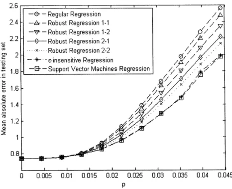
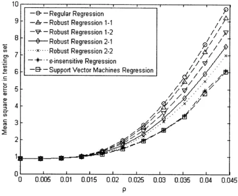
Figure 2-1: The average mean absolute error of the regression estimates according to p. Using this procedure, the average mean absolute error and the average mean squared error of each estimate in the testing set was calculated for values of p between 0 and 0.045. The graphs of these errors according to p can be seen in Figures 2-1 and 2-2. The legends "Robust Regression 1-1", "Robust Regression 1-2", "Robust Regression 1", "Robust Regression 2-2" refer to the robust regression estimates with (p = 1, q = 1), (p = 1, q = 2), (p = 2, q = 1), and (p = 2, q = 2), respectively.

We observe that as p increases, the difference in the out-of-sample performance between the robust and the respective classical estimates increases, with the robust estimates always yielding better results. The support vector and E-insensitive regression estimates performed the best, while the ordering of the other methods in decreasing performance was: Robust 2-2, Robust 2-1, Robust 1-2, Robust 1-1.

The robust regression estimates were also tested using real data from the UCI Machine Learning Repository [3]. Again, the sets were normalized by scaling each one of the vectors containing the data corresponding to an independent variable to make their 2-norm equal to 1. The sizes of the used data sets can be seen in Table 2.1.

The evaluation procedure for each real data set was the following:

* The data set was divided in three sets, the training set, consisting of the 50% of the samples, the validating set, consisting of the 25% of the samples, and the testing set,

IU I I I I

-& - Regular Regression

9 -A,- Robust Regression 1-1

'

- - Robust Regression 1-2

8 - Robust Regression 2-1 /

7 ----....x _{Robust Regression 2-2}

C: - - s-insensitive Regression /

w 6 -E -Support Vector Machines Regression

04

-C5 3

-0 0.005 0.01 0.015 0.02 0.025 0.03 0.035 0.04 0.045

Figure 2-2: The average mean squared error of the regression estimates according to p.

Data set

n

m

Abalone

4177

9

Auto MPG

392

8

Comp Hard

209

7

Concrete

1030

8

Housing

506

13

Space shuttle

23

4

WPBC

46

32

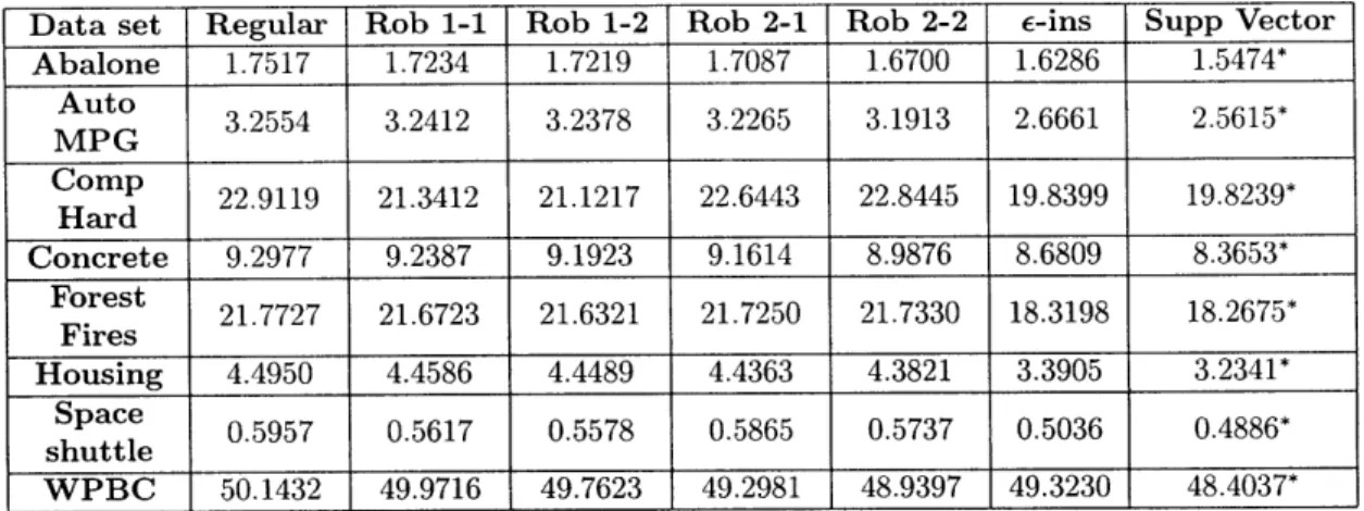
Data set Regular Rob 1-1 Rob 1-2 Rob 2-1 Rob 2-2 E-ins Supp Vector Abalone 1.7517 1.7234 1.7219 1.7087 1.6700 1.6286 1.5474* Auto 3.2554 3.2412 3.2378 3.2265 3.1913 2.6661 2.5615* MPG Comp 22.9119 21.3412 21.1217 22.6443 22.8445 19.8399 19.8239* Hard Concrete 9.2977 9.2387 9.1923 9.1614 8.9876 8.6809 8.3653* Forest 21.7727 21.6723 21.6321 21.7250 21.7330 18.3198 18.2675* Fires Housing 4.4950 4.4586 4.4489 4.4363 4.3821 3.3905 3.2341* Space 0.5957 0.5617 0.5578 0.5865 0.5737 0.5036 0.4886* shuttle WPBC 50.1432 49.9716 49.7623 49.2981 48.9397 49.3230 48.4037*

Table 2.2: Mean absolute error in

the best performance.

testing set for real data sets. * denotes the estimate with

consisting of the rest 25% of the samples. We considered

data set which were selected randomly.

30 different partitions of the

* For each one of the considered partitions of the data set:

- The regular regression estimate based on the training set was calculated.

- The robust regression estimates based on the training set for various values of

p were calculated. For each p, the total prediction error on the validating set

was measured, and the p with the highest performance on the validating set was considered. The prediction error that this p yielded on the testing set was recorded.

* The prediction errors of the estimates under examination were averaged over the par-titions of the data considered.

Parameter c for c-insensitive regression and the support vector machines regression was chosen in the same way as in the artificial data experiments.

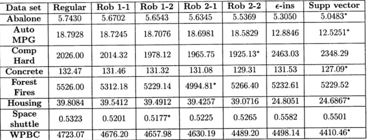
The results of the evaluation process are summarized in Tables 2.2 and 2.3. Under the mean absolute error criterion, the support vector machines are always performing the best. In most cases, the ordering in the out-of-sample experiments is the same as in the artificial data sets. Under the mean squared error criterion, in five out of the eight real data sets, the support vector machines show the best performance, whereas in the rest three data sets, the robust regression estimates yield smaller out-of-sample errors.

Data set Regular Rob 1-1 Rob 1-2 Rob 2-1 Rob 2-2 E-ins Supp vector Abalone 5.7430 5.6702 5.6543 5.6345 5.5369 5.3050 5.0483* Auto 18.7928 18.7245 18.7076 18.6981 18.5829 12.8846 12.5251* MPG Comp 2026.00 2014.32 1978.12 1965.75 1925.13* 2463.03 2348.29 Hard Concrete 132.47 131.46 131.32 131.08 129.31 131.53 127.09* Forest 5526.00 5312.18 5229.14 4994.81* 5266.40 5232.61 5229.52 Fires Housing 39.8084 39.5412 39.4912 39.4257 39.0716 24.8051 24.6867* Space 0.5323 0.5201 0.5177* 0.5225 0.5265 0.5582 0.5501 shuttle WPBC 4723.07 4676.20 4657.98 4630.19 4489.20 4498.14 4410.46*

Table 2.3: Mean squared

the best performance.

error in testing set for real data sets.

*

denotes the estimate with

2.5

Conclusions

Regularization in statistics can be interpreted as the application of robust optimization techniques in classical statistical estimates to provide protection against uncertainty in the data. The robust optimization paradigm offers a more adaptive and comprehensive control of the estimates through the use of various norms in defining uncertainty sets, while, at the same time, providing an insight of why the produced estimates yield improved performance compared to their respective classical ones.

Chapter 3

Support Vector Machines as Robust

Estimators

3.1

Introduction

Vapnik et al. [10] developed Support Vector Machines (SVM), a method which provides classification estimates. Given a set of data (yi, xi), i E {1, 2,...,, n},i E {-1, 1}, xi E Im,

the SVM estimate is the optimal solution to optimization problem

n

min

I

13I2 + p E i

30 o,4 i=1

s.t. ( > 1 - y(13'ziX +o),i E {1,2,...,n} (3.1)

> 0,i E {1,2,...,n},

where p > 0. The term

II3ll2

n

that is as far as possible from the samples and the term p

Z

i=1

samples. Support vector machines classifiers have been very successful in experiments (see Scholkopf [43]). Note that Problem (3.1) has a regularization term 1 3112 in its objective.

The idea of applying Robust Optimization in defining classification estimators has already been explored. Lanckriet, El Ghaoui et al. defined classification estimators by minimizing the worst-case probability of misclassification [34]. The connection of SVM with robustness has already been explored. Shivaswamy et al. propose a second order cone programming problem that defines classifiers that can handle uncertainty [44].

In this chapter, we prove that Support Vector Machines are a particular case of robust optimization estimators (this last fact was also observed independently and simultaneously by Xu, Caramanis, and Mannor [52]). More specifically, in Section 3.2, we prove that the

support vector machines problem, which yields the respective estimate for classification, is the robust counterpart of some nominal problem which classifies binary data as well, and we calculate the relation between the norms of the uncertainty sets and the norm used for the regularization. In Section 3.3, we report on computational results of the Support Vector Machines estimators and their respective classical ones.

3.2

Robust Properties of Support Vector Machines

Given a set of categorical data (yi, xi), yi E {1, -1}, x E Rm, i E {1, 2,... , n}, we define

the separation error S(/, 3o, y, X) of the hyperplane classifier 8Tx + /o = 0, x E Rm, by

n

S(P3, o, Y, X) = ? max(O, 1 - yi(PTx + Qo)), (3.2) i=1 where Y1 X1 Y2 X2 y = , and X =

[

According to Eq. (3.2), an observation (yi, xi) contributes a non-zero quantity to S(3,

3o, y, X) only if 3Txi + 0o < 1, fTxi + /0 > -1, for Yi 1, i = -1, respectively. The amount of the contribution is the distance of 3Txi + o3 from 1, -1, for yi = 1, i -1,

respectively.

The hyperplane which minimizes the separation error is the solution to the optimization problem

min S(P, O0, y, X), (3.3)

which can be expressed as the linear optimization problem

n

mmin

i=l

s.t. yi(PTi + 00) 1 - ,i E {1,2,...,n} (4 > 0,i e {1,2,... ,n}.

Consider the uncertainty set

N3

=

AX R

|Ax

(3.4)

where II* lip is the p-norm.

The robust version of Problem (3.3), which immunizes the computed hyperplane against errors in the independent variables of the data described by the set JN3, is

min max S(8, 30, y, X + AX). (3.5) 1,1o AXEK3

We next prove that under Assumption 2, this robust estimate is equivalent to the support vector machines classification estimate.

Definition 3. The set of data (yi, xi), i E {1, 2,..., n}, is called separable if there exists a hyperplane OTx + Qo = 0, such that for any i E {1, 2,... , n}, y i(3Txi + /o) > 0. Otherwise,

the data set is called non-separable. In this case, for any hyperplane I3TX + /o = 0, there

exists an i E {1, 2,...,n} with yi(3Txi + 3o) < 0.

Assumption 2. The data (yi, xi), i E {1, 2,..., n}, is non-separable.

Theorem 3. Under Assumption 2, Problem (3.5) is equivalent to n

min 1 i +P II Id(p)

,P= i= 1 T

s.t. i > 1 - y(P/Tx + 3o), i E {1, 2,..., n} (3.6)

i 2 0, i E {1,2,...,n},

where d(p) is defined in Eq. (4.3), i.e., I" I*d(p) is the dual norm of II lip.

Proof.

To prove the theorem, we are going to introduce a new set of variables ri, i E {1, 2,..., n}, which will be used to bound each

IIAxillp,

IfAxillp to 7 IAxillp, which determines the uncertainty set.

i=1

Consider

and

R2=

{(AX,r)

x

I AxiIp

1,2,..., n}.

(3.8)

It is clear that the projection of R 2 onto AX is N3. Thus, the inner problem in Eq. (3.5)

can be expressed as

max S(,3, /3o, X + AX),

(AX,r)ER2 (3.9)

which is equivalent to

max max S(, o0, y, X + AX).

rER1 IlAxillprip

Consider the inner maximization problem in Eq. (3.10) max S(, o30, y, X + AX). JAxIllp_<rip (3.10) (3.11)

Since

S(p, Oo, y, X + AX) = max(0, 1 - yi(fT(xi + Axi) + 3o)),

i=1

Problem (3.11) is separable and has separable constraints. Its solution is given by solving

max max(0, 1 - y(P3T(x + Axi) + 3o)). I Ai,_pI<rip

for any i E {1, 2,..., n} and adding the optimal objectives. Observe that:

max _{max(0, 1 - yi(3T(xi + Axi) + 0o)} Jl~xilllrip

= max(0, max (1 - yi(3Txi + /0) - yi TAxi))

IAx zillp <rip

= max(0, 1 - yi(P3Txi

+

(3.12)

max (-yiTAXi)).

We know that:

max (-yi3T Axi))

IIAxl pfrip - min fTA , IIAxlp<rip max /3TA xi, Jlaaxillp<rip min fT Ax = -riplll3

11q,

and

max

= ripll

pIq.

IlAxillp<rip

Consequently,

max (-yiTA i_{) = riPIlllq,} IlA illprip

and

max _{max(0, 1 - yi(PT(x + Axi) + ,o))}

IlAxi lp<rip

= max(0, 1 - yi(3Txi + 0o) +

max

IlA illp<riP(-yiTAXi))

=

max(0,

+

3o) +

ripll

1

q)

is the optimal objective of Problem (3.12). Thus, the optimal objective of Problem (3.11) is

n

Smax(O,

i=1

Given this observation, Problem (3.10) is equivalent to

max

max(O,

- y,(PTxi

00)

ripl

/

_11q).

(3.13)

To solve Problem (3.13), we find an upper bound for its objective value and then, we construct if Yi = 1,

an r which achieves this upper bound.

Since

max(O, 1 - yi(3Txi + 3o) + ripI 3 11q)

<

we conclude that for r E R

max(0, 1 - yi(3Tix + 00)

+P

i=1

- max(O, 1 - yi(3Txi + s3)) + riPI 0

Iq

n

-

S(0,

3o,

y, X)

+

rPpl|/

|q

Pl l

q.

i=1

Using Assumption 2, the data is non-separable, and thus, there exists an im E {1, 2,..., n}

such that yim (P3Txim + 0o) < 0. We have:

1 - yi (P3TziXm+ ) > 0,

and

PII11

max(0, 1 - y2 (3Txi + 3o) + riPI 01q)

n

= max(0, 1- yi(3Txi

+

3o))

_liq

i=l,i im

n

=

max(0, 1

-

_{y~i(Oxi + 0o)) + PJIll = S(A 0o, y, X) + PI~}

_f3II

Thus, the optimal objective value of Problem (3.13) is S(P3, fo, y, X) + pl

fl

Iq and a robust

min S(3,

Oo,

PIIP

which is equivalent to Problem (3.6). O As Theorem 3 states, the support vector machines estimate is a robust optimization estimate, attempting to provide protection against errors in the independent variables.

3.3

Experimental Results

To compare the performance of the Support Vector Machines to the performance of their respective nominal estimators, we conducted experiments using artificial, as well as real data sets. To solve all the convex problems needed to compute the estimates, we used SeDuMi [36], [48].

The artificial data set used to evaluate the support vector machines classifier was generated in the following way:

* A set of 100 points in RI3 obeying the multivariate normal distribution with mean [1, 0, 0]T and covariance matrix -.

_I3

matrix. The points were associated with y = 1, and added to the data set.

* A set of 100 points in R3 obeying the multivariate normal distribution with mean [0, 1, O]T and standard deviation

-I3

y = -1, and added to the data set.

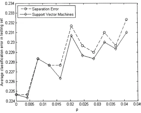
The performance of the separation error estimate and the support vector machines esti-mate was measured for values of p ranging between 0 and 0.045 using the generated data set and the same procedure as in the regression artificial data case described in Chapter 2. The results are summarized in Figure 3-1. The performance metric used was the classification error of the estimate. We observe that the support vector machines estimate, which is the

0.234 a ) o 0.232 / 0 0.231 -Z 0.23 -._ 0.229 / .• 0.228 S0.227 ,) a 0.226 0.225 0.224 i 0 0.005 0.01 0.015 0.02 0.025 0.03 0.035 0.04 0.045 P

Figure 3-1: The average classification error of the classification estimates according to p.

robust version of the separation error estimate, yields a smaller error for most of the values of p, confirming the effectiveness of the robustness and regularization procedure.

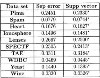
The classification estimates were also tested using real data from the UCI Machine Learn-ing Repository [3]. The procedure followed was the same as in the regression estimates case described in Chapter 2, and the performance metric applied was the classification error. The sizes of the used data sets can be seen in Table 3.1. The results are summarized in Table 3.2. The support vector machines estimate yields better results than the separation error estimate in all cases. The maximum improvement is obtained in the "Lenses" set, where the support vector machines estimate, which is characterized by the robust optimization and regularization ideas, is 6.25% better than the classical estimate.

3.4

Conclusions

Support Vector Machines for classification is a particular case of an estimator defined using the robust optimization paradigm. We proved theorems that facilitate the choice of the norm and the coefficient used in regularization based on the structure and the size of the considered uncertainty sets. The robust estimator shows improved performance in artificial and real data sets compared to its respective nominal one.

Data set

n

m

Pima

768

8

Spam

4601

57

Heart

270

13

Ionosphere

351

33

Lenses

24

5

SPECTF

267

44

TAE

151

5

WDBC

569

30

Yeast

1484

8

Wine

178

13

Table 3.1: Sizes of real data sets for classification.

Data set Sep error Supp vector Pima 0.2451 0.2330* Spam 0.0779 0.0744* Heart 0.1676 0.1627* Ionosphere 0.1496 0.1481* Lenses 0.2667 0.2500* SPECTF 0.2505 0.2413* TAE 0.3311 0.3184* WDBC 0.0469 0.0445* Yeast 0.1440 0.1395* Wine 0.0330 0.0326*

Table 3.2: Classification error in testing set for real data sets. * denotes the estimate with the best performance.

Chapter 4

Robust Logistic Regression

4.1

Logistic Regression

Logistic regression is a widely used method for analysing categorical data, and making pre-dictions for them. Given a set of observations (yi,

xi),

classical logistic regression calculates the maximum likelihood estimate for the parameter (/3, 3o) E Rm+_{1 of the logistic regression model (see Ryan [40], Hosmer [28])}

exp(/Tx + 3o)

Pr[Y = 1X = X] = expT + / (4.1) 1 + exp(O3Tx + 30) (4.1) where Y E {0, 1} is the response variable determining the class of the sample and X E Rm is the independent variables vector.

Very frequently, the observations used to produce the estimate are subject to errors. The errors can be present in either the independent variables, in the response variable, or in both. For example, in predicting whether the financial condition of a company is sound, the economic indices of the company used to make the prediction might have been measured with errors. In predicting whether a patient is going to be cured from a disease given several medical tests they undertook, the response variable demonstrating whether the patient was indeed cured might contain errors.

The presence of errors affects the estimate that classical logistic regression yields and makes the predictions less accurate. It is desirable to produce estimates that are able to make accurate predictions even in the presence of such errors.

In this thesis, robust optimization techniques are applied in order to produce new robust estimates for the logistic regression model that are more immune to errors in the observations' data. The contributions achieved include:

1. New notions of robust logistic regression when the estimates are immunized against errors in only the independent variables, in only the response variable, and in both the independent and the response variables are introduced.

2. Efficient algorithms based on convex optimization methods on how to compute these robust estimates of the coefficients (0, iO) in Eq. (4.1) are constructed.

3. Experiments in both artificial and real data illustrate that the robust estimates provide superior out-of-sample performance.

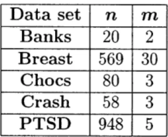
The structure of the chapter is as follows. In Sections 4.2, 4.3, and 4.4, the methodology of computing robust logistic regression estimates that are protected against errors in their independent variables, in their response variable, or in both respectively is outlined. In Section 4.5, the performance of the proposed algorithms in comparison with the classical logistic regression for both artificial, and real data sets is reported.

4.2

Robust logistic regression under independent

vari-ables uncertainty

Given a set of observations (yi, ji), i E {1, 2,..., n}, we assume that the true value of the independent variables of the observations is xi + Axi, where the p-norm of Axi is bounded

above by some parameter p, that is Il Axilp < p.

Let X be the matrix in which row i is vector xi, AX be the matrix in which row i is vector Ax, and y be the vector whose i-th coordinate is yi, i = 1, 2,...,n. Let function

P(y, X,

1,

n

P(y, X,

3,

i=1

Let

d(p) = p > 1. (4.3)

p-i'

We also define that d(1) = oc and d(oo) = 1. Note that * I d(p) is the dual norm of * lip.

Let