Supervised Extraction of Diagnosis Codes from
EMRs: Role of Feature Selection, Data Selection,
and Probabilistic Thresholding
Anthony Rios
Department of Computer Science University of Kentucky, Lexington, KY
Ramakanth Kavuluru
∗Division of Biomedical Informatics, Dept. of Biostatistics Department of Computer Science
University of Kentucky, Lexington, KY [email protected]
Abstract—Extracting diagnosis codes from medical records is a complex task carried out by trained coders by reading all the documents associated with a patient’s visit. With the popularity of electronic medical records (EMRs), computational approaches to code extraction have been proposed in the recent years. Machine learning approaches to multi-label text classification provide an important methodology in this task given each EMR can be associated with multiple codes. In this paper, we study the the role of feature selection, training data selection, and probabilistic threshold optimization in improving different multi-label classification approaches. We conduct experiments based on two different datasets: a recent gold standard dataset used for this task and a second larger and more complex EMR dataset we curated from the University of Kentucky Medical Center. While conventional approaches achieve results comparable to the state-of-the-art on the gold standard dataset, on our complex in-house dataset, we show that feature selection, training data selection, and probabilistic thresholding provide significant gains in performance.
I. INTRODUCTION
Extracting codes from standard terminologies is a regular and indispensable task often encountered in medical and healthcare fields. Diagnosis codes, procedure codes, cancer site and morphology codes are all manually extracted from patient records by trained human coders. The extracted codes serve multiple purposes including billing and reimbursement, quality control, epidemiological studies, and cohort identification for clinical trials. In this paper we focus on extracting international classification of diseases, clinical modification, 9th revision (ICD-9-CM) diagnosis codes from electronic medical records (EMRs), and the application of supervised multi-label text classification approaches to this problem.
Diagnosis codes are the primary means to systematically encode patient conditions treated in healthcare facilities both for billing purposes and for secondary data usage. In the US, ICD-9-CM (just ICD-9 henceforth) is the coding scheme still used by many healthcare providers while they are required to comply with ICD-10-CM, the next and latest revision, by October 1, 2014. Regardless of the coding scheme used, both ICD code sets are very large, with ICD-9 having a total of 13,000 diagnoses while ICD-10 has 68,000 diagnosis codes [1] and as will be made clear in the rest of the paper, our methods will also apply to ICD-10 extraction tasks. ICD-9
∗Corresponding author
codes contain 3 to 5 digits and are organized hierarchically: they take the form abc.xy where the first three character part before the period abc is the main disease category, while the x and y components represents subdivisions of the abccategory. For example, the code 530.12is for the condition reflux esophagitisand its parent code530.1is for the broader condition of esophagitis and the three character code 530 subsumes all diseases of esophagus. Any allowed code assignment should at least assign codes at the category level (that is, the first three digits). At the category levels there are nearly 1300 different ICD-9 codes.
The process of assigning diagnosis codes is carried out by trained human coders who look at the entire EMR for a patient visit to assign codes. Majority of the artifacts in an EMR are textual documents such as discharge summaries, operative reports, and progress notes authored by physicians, nurses, or social workers who attended the patient. The codes are assigned based on a set of guidelines [2] established by the National Center for Health Statistics and the Centers for Medicare and Medicaid Services. The guidelines contain rules that state how coding should be done in specific cases. For example, the signs and symptoms (780-799) codes are often not coded if the underlying causal condition is determined and coded. Given the large set of possible ICD-9 codes and the need to carefully review the entire EMR, the coding process is a complex and time consuming process. Hence, several attempts have been made to automate the coding process. However, computational approaches are inherently error prone. Hence, we would like to emphasize that automatic medical coding systems, including our current attempt, are generally not intended to replace trained coders but are mainly motivated to expedite the coding process and increase the productivity of medical record coding and management.
In this paper, we explore supervised text classification approaches to automatically extract ICD-9 codes from clinical narratives using two different datasets: a gold standard dataset created for the BioNLP 2007 shared task [3] by researchers af-filiated with the Computational Medicine Center (CMC1) and a
new dataset we curated from in-patient EMRs at the University of Kentucky (UKY). The BioNLP dataset (henceforth referred to as the CMC dataset) is a high quality, but relatively small, dataset of clinical reports that covers the pediatric radiology
domain. The gold standard correct codes are provided for each report. To experiment with a more realistic dataset, we curated the UKY dataset that covers more codes from a random selection of in-patient EMRs, where the correct codes are obtained per EMR from trained coders in the medical records office at UKY.
In supervised classification, multi-label problems are gen-erally transformed into several multi-class (where each artifact belongs to a single class) or binary classification problems. In this effort, we explore these different transformation techniques with different base classifiers (support vector machines, naive Bayes, and logistic regression). Large label sets, high label cardinality (number of labels per artifact), class imbalance, inter-class correlations, large feature sets are some of the factors that negatively affect performance in multi-label clas-sification problems. We experiment with different state-of-the-art feature selection, training data selection, classifier chaining, and probabilistic thresholding approaches to address some of these issues. We achieve comparable results to the state-of-the-art on the CMC dataset. Our experiments reveal how the differences in the nature of our two datasets significantly affect the performance of different supervised approaches. Our ablation experiments also demonstrate the utility of training data selection, feature selection, and threshold optimization on the overall performance of our best classifiers and point to the potential of these approaches in the general problem of computational code extraction.
The rest of the paper is organized as follows: In Section II we discuss related work on diagnosis code extraction and provide background on multi-label classification approaches. We elaborate on the two different datasets used in Section III. In Section IV, we present details of different text classification algorithms and different learning components used in our experiments. After a brief discussion of evaluation measures in Section V, we present our results in Section VI.
II. RELATEDWORK ANDBACKGROUND
In this section we discuss related work on prior efforts in extracting ICD-9 codes and briefly discuss the general background for multi-label classification techniques.
Several attempts have been made to extract ICD-9 codes from clinical documents since the 1990s. Advances in natural language and semantic processing techniques contributed to a recent surge in automatic extraction. de Lima et al. [4] use a hierarchical approach utilizing the alphabetical index provided with the ICD-9-CM resource. Although completely unsupervised, this approach is limited by the index not being able to capture all synonymous occurrences and also the inability to code both specific exclusions and other condition specific guidelines. Gunderson et al. [5] extracted ICD-9 codes from short free text diagnosis statements that were generated at the time of patient admission using a Bayesian network to encode semantic information. However, in the recent past, concept extraction from longer documents such as discharge summaries has gained interest. Especially for ICD-9 code extraction, recent results are mostly based on the systems and the CMC dataset developed for the BioNLP workshop shared task on multi-label classification of clinical texts [3] in 2007.
The CMC dataset consists of 1954 radiology reports aris-ing from outpatient chest x-ray and renal procedures and is observed to cover a substantial portion of pediatric radiology activity. The radiology reports are also formatted in XML with explicit tags for history and impression fields. Finally, there are a total of 45 unique codes and 94 distinct combinations of these codes in the dataset. The dataset is split into training and testing sets of nearly equal size where example reports for all possible codes and combinations occur in both sets. This means that all possible combinations that will be encountered in the test set are known ahead of time. The top system obtained a micro-average F-score of 0.89 and 21 of the 44 participating systems scored between 0.8 and 0.9. Next we list some notable results that fall in this range obtained by various participants and others who used the dataset later. The techniques used range from completely handcrafted rules to fully automated machine learning approaches. Aronson et al. [6] adapted a hybrid MeSH term indexing program MTI that is in use at the NLM and included it with SVM andknearest neighbor classifiers for a hybrid stacked model. Goldstein et al. [7] applied three different classification approaches -traditional information retrieval using the search engine library Apache Lucene, Boosting, and rule-based approaches. Cram-mer et al. [8] use an online learning approach in combination with a rule-based system. Farkas and Szarvas [9] use an interesting approach to induce new rules and acquire synonyms using decision trees. N´ev´eol et al. [10] also model rules based on indexing guidelines used by coders using semantic predications to assign MeSH heading-subheading pairs to in-dexing biomedical articles. A recent attempt [11] also exploits the hierarchical nature of the the ICD-9-CM terminology to improve the performance achieving comparable performance to the best scores achieved during the competition.
Next, we provide a brief review of the background and state-of-the-art in multi-label classification, the general prob-lem of choosing multiple labels among a set of possible labels for each object that needs to be classified. A class of approaches called problem transformation approaches con-vert the multi-label problem into multiple single-label clas-sification instances. A second class of methods adapts the specific algorithms for single-label classification problems to directly predict multiple labels. Both problem transformation and algorithm adaptation techniques are covered in this recent survey by [12]. Recent attempts in multi-label classification also consider label correlations [13]–[15] when building a model for multi-label data. An important challenge in problems with a large number of labels per document is to decide the number of candidates after which candidate labels should be ignored, which has been recently addressed by calibrated rank-ing [16] and probabilistic thresholdrank-ing [17]. Feature selection is an important aspect when building classifiers using machine learning. We request the readers to refer to Forman [18] for a detailed comparative analysis of feature selection methods. Combining the scores for each feature using different fea-ture selection methods has also been applied to multi-label classification [19]. When dealing with datasets with class imbalance, methods such as random under/over-sampling, syn-thetic training sample generation, and cost-sensitive learning were proposed (see [20] for a survey). In contrast with these approaches, Sohn et al [21] propose an alternative Bayesian approach to curate customized optimal training sets for each
label. In the next section, we discuss the characteristics of the two datasets used in this paper.
III. DATASETS
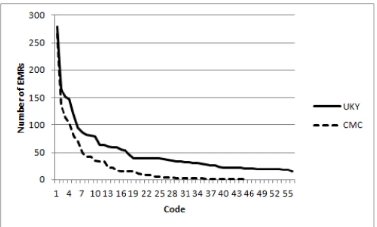
We already introduced the CMC dataset in Section II when discussing related work. Here we will give some additional details to contrast it with the our UKY hospital dataset. From the 1954 reports in the CMC dataset, 978 are included in the training dataset with their corresponding ICD-9 codes; the remaining documents form the testing set. All labels sets that occur in the testing set occur at least once in the training dataset. In Figure 1, we show how many times each of the 45 ICD-9 codes occurred in the training set. We can see that 75% of the codes appear less than 50 times in the training set. Almost 50% of the 45 labels appear less than ten times. For each instance in the CMC dataset there are two fields that contain textual data, ‘clinical history’ and ‘impression’. Clinical history field contains textual information entered by a physician before a radiological procedure about the patient’s history. The impression field contains textual entered by a radi-ologist after the radiological procedure about his observations of the patient’s condition as obtained from the procedure. Many of the textual entries contained in these two fields are very short. An example of the clinical history field is “22 month old with cough.” The corresponding impression is just one word “normal.” The average size of a report is 21 words.
We also built a second dataset to study code extraction at the EMR level. We created a dataset of 1000 clinical document sets corresponding to a randomly chosen set of 1000 in-patient visits to the UKY Medical Center in the month of February, 20122 We also collected the ICD-9 codes for these EMRs assigned by a trained coder at the UKY medical records office. Aggregating all billing data, this dataset has a total of 7480 diagnoses leading to 1811 unique ICD-9 codes. Recall, that the ICD-9 codes have the formatabc.xywhere the first three dig-its abccapture the category. Using the (category code, label, count) representation the top 5 most frequent categories are (401, essential hypertension, 325), (276, Disorders of fluid electrolyte and acid-base balance, 239), (305, nondependent abuse of drugs, 236), (272, disorders of lipoid metabolism, 188), and (530, diseases of esophagus, 169). The average number of codes is 7.5 per EMR with a median of 6 codes. There are EMRs with only one code, while the maximum number assigned to an EMR is 49 codes. For each in-patient visit, the original EMR consisted of several documents, some of which are not conventional text files but are stored in the RTF format. Some documents, like care flowsheets, vital signs sheets, ventilator records were not considered for this analysis. We have a total of 5583 documents for all 1000 EMRs. On an average there are 5.6 textual documents per EMR, but considering only those authored by physicians, there are 2.8 documents per EMR.
Since many of the 1811 codes in the UKY dataset have very few examples, we decided to consider extracting codes at the fourth digit level. That is, all codes of the form abc.xy
for different ‘y’are mapped to the four digit code abc.x. With this mapping we had 1410 unique codes. Note the the 2This dataset has been approved by the UKY IRB for use in research projects (protocol #12-0139-p3h).
Fig. 1. Distribution of ICD-9 code counts in the datasets. Number of EMRs on the Y-axis and the codes arranged in descending order of frequencies on the X-axis
average number of codes per EMR even when we collapsed the fifth digit is still 7.5 (the same value as for the case of full five digit codes). This is because, in general, an EMR does not have two codes that differ at the fifth digit, which captures the finest level of classification. The average size of each EMR (that is, of all textual documents in it) in the UKY dataset is 2088 words. Even when truncated to 4 digits, there were still many codes that had too few examples to apply supervised methods. Hence we resorted to using 56 codes (at that fourth digit level) that had at least 20 EMRs in the dataset; the number of unique combinations of these 56 codes is about 554. After removing those EMRs that did not have any of these frequently occurring 56 codes, we are left with 827 EMRs in the dataset. We randomly selected and removed 100 examples from the dataset to be used for testing and the remaining 727 EMRs formed the training dataset. The distribution of the 4 digit code counts in the training set can be seen in Figure 1.
Label-cardinalityis the average number of codes per report (or EMR in the UKY dataset). To use consistent terminology we refer to the single reports in the CMC dataset as EMRs that consist of just one document. Let mbe the total number of EMRs andYi be the set of labels for the i-th EMR. Then
we have Label-Cardinality= 1 m m X i=1 |Yi|.
The CMC training dataset had a label cardinality of1.24and the UKY dataset has a label cardinality of3.86. Another useful statistic that describes the datasets is label-density, which divides the average number of codes per EMR by the total number of unique codes q. We have
Label-Density=1 q · 1 m m X i=1 |Yi|.
The label-density for the CMC training dataset is0.03and for the UKY dataset is0.06. Unlike label-cardinality, label-density also takes into account the number of unique labels possible. Two datasets with the same label cardinality can have different label densities and might need different learning approaches tailored to the situations. Intuitively, in this case, the dataset with the smaller density is expected to have fewer training examples per label.
As we can see, the datasets have significant differences: the CMC data set is coded by three different coding companies and final codes are consolidated from these three different extractions. As such, it is of higher quality compared to the UKY dataset which is coded by only one trained coder from the UKY medical records office. On the other hand, the CMC dataset does not have the broad coverage of the UKY dataset, which models a more realistic dataset at the EMR level. The CMC dataset only includes radiology reports and has 45 codes with 94 code combinations and has on an average 21 words per EMR. In contrast, even with the final set of 56 codes (at the four digit level) that have at least 20 examples that we use for our experiments, the number of combinations for the UKY dataset is 554 with the average EMR size two orders of magnitude more than the average for the CMC dataset.
IV. MULTI-LABELTEXTCLASSIFICATIONAPPROACHES In this section, we describe the methods we employ for multi-label classification to extract ICD-9 codes from both the datasets. Our core methods primarily use the problem transfor-mation approach where the multi-label classification problem is converted into multiple binary classification problems. We also use different approaches that take into account label correlations expressed in the training data. Besides this basic framework, we utilize feature selection, training data selection, and probabilistic thresholding as additional components of our classification systems. One of our goals is to see how all these components and transformation approaches perform on the two different datasets we discuss (Section III).
We used the Java based packages Weka [22] and Mu-lan [23] for our classification experiments. Next, we describe different components of our classification approaches.
A. Document Features
We used unigram and bigram counts as features. Stop words (determiners, prepositions, and so on) were removed from the unigram features. Since unigrams and bigrams are syntactic features, we also used semantic features such as
named entities and binary relationships (between named en-tities) extracted from text, popularly called semantic predica-tions, as features.
To extract named entities and semantic predications, we used software made available through the Semantic Knowledge Representation (SKR) project by the National Library of Medicine (NLM). The two software packages we used were MetaMap and SemRep. MetaMap [24] is a biomedical named entity recognition program that identifies concepts from the Unified Medical Language System (UMLS) Metathesaurus, an aggregation of over 160 biomedical terminologies. When MetaMap outputs different named entities, it associates a confidence score in the range from 0 to 1000. We only used concepts with a confidence score of at least 700 as features. Each of the concepts extracted by MetaMap also contains a field specifying if the concept was negated (e.g., “no evidence of hypertension”). We used negated concepts that capture the absence of conditions/symptoms as different features from the original concepts. We used SemRep, a relationship extraction program developed by Thomas Rindflesch [25] and team at the NLM that extracts semantic predications of the form
C1 → relationT ype → C2 where C1 and C2 are two different biomedical named entities and relationT ype ex-presses a relation between them (e.g., “TamoxifentreatsBreast Cancer”). Because predication extraction is made by making calls using the Web API provided by SKR, we only used predications as features for the de-identified CMC dataset and not for the UKY dataset. If there is more than one document in an EMR, features are aggregated from all documents authored by a physician.
B. Base Classifiers and Problem Transformation Approaches for Multi-Label Classification
For the binary classifiers for each label, we experimented with three base classifiers: Support Vector Machines (SVMs), Logistic Regression (LR), and Multinomial Naive Bayes (MNB). We used the MNB classifier that is made available as part of the Weka framework. For LR, we used LibLIN-EAR [26] implementation in Weka and for SVMs we used LibSVM [27] in Weka.
We experimented with four different label multi-label problem transformation methods:binary relevance, copy transformation, ensemble of classifier chains, andensemble of pruned label sets.
Let T be the set of labels and let q = |T|. Binary relevance learnsqbinary classifiers, one for each label inT. It transforms the dataset intoq separate datasets. For each label Tj, we obtain the dataset for the corresponding binary classifier
by considering each document–label-set pair (Di,Yi) and
generating the document-label pair (Di, Tj) when Tj ∈ Yi
and generating the pair (Di,¬Tj) when Tj 6∈ Yi. When
predicting, the labels are ranked based on their score output by the corresponding binary classifiers and the top k labels are considered as the predicted set for a suitable k. The copy transformation transforms multi-label data into single-label data. Let T = {T1, . . . , Tq} be the set of q possible
labels for a given multi-label problem. Let each document Dj ∈ D, j = 1, . . . , m, have a set of labels Yj ⊆ T
associated with it. The copy transformation transforms each document–label-set pair (Dj,Yj) into |Yj| document–label
pairs (Dj, Ts), for all Ts ∈ Yj. After the transformation,
each input pair for the classification algorithm will only have one label associated with it and one can use any single-label method for classification. The labels are then ranked based on the score given from the classifier when generating predictions. We then take the top k labels as our predicted label set.
One of the main disadvantages of the binary relevance and copy transformation methods is that they assume label independence. In practical situations, there can be dependence between labels where labels co-occur very frequently or where a label occurs only when a different label is also tagged. Classifier chains [13], based on the binary relevance trans-formation, try to account for these dependencies that the basic transformations cannot. Like binary relevance, classifier chains transform the dataset into q datasets for binary classification per each label. But they differ from binary relevance in the training phase. Classifier chains loop through each dataset in some order, training each classifier one at a time. Each binary classifier in this order will add a new Boolean feature to the subsequent binary classifier datasets to be trained next. For
further details of the chaining approach and the ensemble of chains modification that overcomes dependence on the chaining order, we request the reader to refer the paper by Read et al. [13].
While ensemble of classifier chains overcomes some of the issues involving the ordering of chaining, the more labels in the training set, the larger the number of ensembles one needs in the training set. Another multi-label classification method that takes label correlations into account is the pruned label sets approach [15]. In this approach, a multi-label problem is transformed into a multi-class problem by representing combi-nations of different labels as new classes. Let each document Dj∈D,j= 1, . . . , m, have a set of labelsYj ⊆Tassociated
with it. Pruned sets will treat each unique set of labels among
Yj as a single class and corresponding EMRs as training
examples for that class. Only combinations whose training data counts are above a user chosen threshold are converted into new classes. For infrequent combinations, smaller subsets of these combinations that are more frequent are converted into new classes with training examples obtained from the corresponding combinations. To overcome the issue of not being able to predict subsets of very frequent combinations (since they are already converted into separate classes) in the basic pruned sets approach, using an ensemble approach, several pruned set classifiers are trained on random subsets of the original training data with final predictions made using a voting approach (please see [15] for more specific details).
C. Feature Selection
An important issue in classification problems with a large number of number of classes and features is that the features most relevant in classifying one class from the rest might not be the same for every class. Furthermore, many features are either redundant or irrelevant to the classification tasks at hand. In the domain of text classification, Bi-Normal Separation (BNS) score was observed to result in best performance in most situations among a set of 12 feature selection methods applied to 229 text classification problems [18]. We employ this feature scoring method for our current effort. Let T = {T1, . . . , Tq} be the set of q possible labels. For each label Ti ∈ T and for each feature, we calculate the number of
true positives (tp) and false positives (f p) with respect to that feature – tp is the number of training EMRs (with label Ti)
in which the feature occurs. Similarly, f p is the number of negative examples forTi in which the feature occurs. Letpos
andnegbe the total number of positive and negative examples forTi, respectively. WithF−1denoting the inverse cumulative
probability function for the standard normal distribution, we define the BNS score of a given feature for a particular class as BN S=|F−1(tpr)−F−1(f pr)| where tpr= tp pos andf pr= f p neg.
Because F−1(0)is undefined, we set tpr andf pr to 0.0005
when tpor f p are equal to zero.
For each of the q binary classification problems, we pick the top k ranked features for each label. In our experiments k = 8000gave the best performance out of a total of 68364
features for the UKY dataset. The number of features was very small for the CMC dataset, a total of 2296 features, feature selection did not improve the performance.
D. Greedy ‘Optimal’ Training Data Selection
In the case of multi-label problems with a large number of classes, the number of negative examples is overwhelmingly larger than the number of positive examples for most labels. We experimented with the synthetic minority oversampling approach [28] for the positive examples which did not prove beneficial for our task. Deviating from the conventional ran-dom under/over-sampling approaches, we adapted the ‘opti-mal’ training set (OTS) selection approach used for medical subject heading (MeSH terms) extraction from biomedical abstracts by Sohn et al. [21]. The OTS approach is a greedy Bayesian approach that under-samples the negative examples to select a customized dataset for each label. The greedy selection is not technically optimal but we stick with the terminology in [21] for clarity. The method for finding OTS is described in Algorithm 1. Intuitively, the method ranks negative examples according to their similarity to positive examples and iteratively selects negative examples according to this ranking and finally selects the negative subset that offers the best performance on a validation set for that label.
Algorithm 1 Optimal Training Set Selection
1: for allBinary datasets B1 toBq do
2: Move 20% of the positive examples and 20% of the negative examples fromBito a validation dataset (Vi). 3: Put the remaining positive examples into a smaller
training dataset (ST Si).
4: Score the remaining negative examples inBiaccording
to their similarity with positive examples. 5: Initialize snapshot variablek= 1
6: while Bi is not emptydo
7: Remove the top10% scored negative examples in Bi and add them to ST Si.
8: Record the snapshot of the current training set, ST Sik=ST Si.
9: Build a binary classifier fori-th code with training datasetST Sk
i and record the F1.5 score onVi. 10: k=k+ 1
11: Set the optimal training setOT S= the snapshotST Sk i
with the highest F1.5 score.
Here we describe how to compute the score for negative examples. Since we want to select those negative examples that are the most difficult to distinguish from the positive examples, for a given negative training example Dj, we would like
our score to be proportional to P(positive|Dj). Using Bayes
theorem, this quantity can be shown (see the online appendix A of [21]) to monotonically increase with the following score function Score(Dj) =ln P(D j|positive) P(Dj|negative) ,
whereP(Dj|positive)is the probability estimate of document Dj given the class is positive, which is estimated using Q
iP(wi|positive)where wis are the unigrams in Dj. Each P(wi|positive)is estimated using counts ofwiin the positive
examples in the training data. Similarly, P(Dj|negative) is
also estimated. The measure we use for assessing the perfor-mance of each STS on the validation set in algorithm 1 is the traditional Fβ measure withβ = 1.5. We choseF1.5over
the traditional balanced F1 measure to give more importance
to recall since the main utility of code prediction is to assist trained coders. Our adaptation of Sohn et al.’s method differs from the original approach in that we don’t resort to the leave-one-out cross validation and instead use a validation set to select the OTS. We also use the naive Bayes assumption for estimates ofP(Dj|positive)involving terms for unigrams that
occur in the document.
E. Probabilistic Thresholding of Number of Labels
In multi-label classification, it is also important to consider effect of the number of labels predicted per document on the performance of the approaches used. A straightforward (and the default approach in many implementations) is to predict all labels whose base binary classifiers predict them with posterior probabilities > 0.5. This could lead to more labels than is actually the case or fewer labels than the actual number. A quick fix that many employ is to pick a threshold of top r (r-cut) labels where the r picked is the one that maximizes the example-based F-score (see Section V) on the training data. However, using this method always results in the same number of labels for each document in the testing set. We used an advanced thresholding method, Multi Label Probabilistic Threshold Optimizer [17] (MLPTO), for choosing a different number of labels per EMR that changes for each EMR instance. The optimizer we employed uses 1−(Example-Based-F-score) as the loss function and finds the r that minimizes the expected loss function across all possible example-based contingency tables for each instance. For specific details of this strategy, please see [17].
V. EVALUATIONMEASURES
Before we discuss our findings, we establish notation to be used for evaluation measures. Since the task of assigning multiple codes to an EMR is the multi-label classification problem, there are multiple complementary methods [29] for evaluating automatic approaches for this task. Recall that Yi, i= 1, . . . , m, is the set of correct labels in the dataset for the i-th EMR, wheremis the total number of EMRs. LetZibe the
set of predicted labels for the i-th EMR. The example-based precision, recall, and F-score are defined as
Pex= 1 m m X i=1 |Yi∩Zi| |Zi| , Rex = 1 m m X i=1 |Yi∩Zi| |Yi| , andFex = 1 m m X i=1 2|Yi∩Zi| |Zi|+|Yi| , respectively.
For each labelTj in the set of labels T being considered,
we have label-based precision P(Tj), recall R(Tj), and
F-scoreF(Tj)defined as P(Tj) = T Pj T Pj+F Pj , R(Tj) = T Pj T Pj+F Nj , andF(Tj) = 2P(Tj)R(Tj) P(Tj) +R(Tj) ,
whereT Pj,F Pj, and F Nj are true positives, false positives,
and false negatives, respectively, of label Tj. Given this, the
label-based macro average F-score is
Macro-F= 1 |T| |T| X j=1 F(Tj).
The label-based micro precision, recall, and F-score are defined as Pmic= P|T| j=1T Pj P|T| j=1(T Pj+F Pj) , Rmic= P|T| j=1T Pj P|T| j=1(T Pj+F Nj) , and Micro-F= 2P mic·Rmic Pmic+Rmic,
While the macro measures consider all labels as equally important, micro measures tend to give more importance to labels that are more frequent. This is relevant for our dataset because we have a very unbalanced set of label counts (see Figure 1) and in such cases micro measures are considered more important.
VI. RESULTS ANDDISCUSSION
In this section we present the results we obtain on both datasets and assess the role of different components of the learning approaches we explored in Section IV.
A. CMC Dataset Results
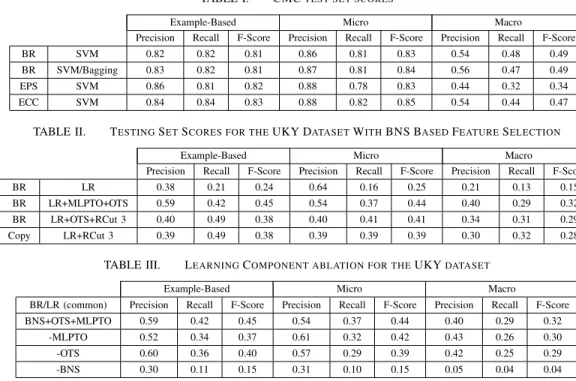
The best results on the CMC dataset were obtained using unigrams and named entity counts (without any weighting) as features and SVMs as the base classifiers. Here, we present the results when using binary relevance (BR), ensemble of classifier chains (ECC), and ensemble of pruned sets (EPS) problem transformation methods. We also used SVMs with bagging to compare BR with the more complex ensemble approaches, ECC and EPS, that take label dependencies into account. In Table I, we can see that the best performing classi-fier is the ensemble of classiclassi-fier chains with an F-score of 0.85. It is interesting to see that BR with bagging also performed reasonably well. For the CMC competition, the micro F-score was the measure used for comparing relative performances of contestants. The mean score in the competition was 0.77 with a standard deviation of 0.13. The best performing method was able to achieve a 0.90 micro F-score.
There were many instances in the CMC dataset where our methods did not predict any codes. We experimented with using an unsupervised approach to generate predictions for those examples: we generated named entities using MetaMap for each of these documents that did not have any predic-tions. We mapped these entities to ICD-9-CM codes via a knowledge-based mapping approach [30] that exploits the graph of relationships in the UMLS Metathesaurus (which also includes ICD-9-CM). If MetaMap generated a concept that got mapped to an ICD-9 code we trained on, we used that ICD-9 code as our prediction. We were able to increase our best F-Score from using ECC from 0.85 to 0.86 using this method. Also, while we don’t report the results for when we added semantic predications as features, the results were comparable with no major improvements. Feature selection,
TABLE I. CMCTEST SET SCORES
Example-Based Micro Macro
Precision Recall F-Score Precision Recall F-Score Precision Recall F-Score
BR SVM 0.82 0.82 0.81 0.86 0.81 0.83 0.54 0.48 0.49
BR SVM/Bagging 0.83 0.82 0.81 0.87 0.81 0.84 0.56 0.47 0.49
EPS SVM 0.86 0.81 0.82 0.88 0.78 0.83 0.44 0.32 0.34
ECC SVM 0.84 0.84 0.83 0.88 0.82 0.85 0.54 0.44 0.47
TABLE II. TESTINGSETSCORES FOR THEUKY DATASETWITHBNS BASEDFEATURESELECTION
Example-Based Micro Macro
Precision Recall F-Score Precision Recall F-Score Precision Recall F-Score
BR LR 0.38 0.21 0.24 0.64 0.16 0.25 0.21 0.13 0.15
BR LR+MLPTO+OTS 0.59 0.42 0.45 0.54 0.37 0.44 0.40 0.29 0.32 BR LR+OTS+RCut 3 0.40 0.49 0.38 0.40 0.41 0.41 0.34 0.31 0.29 Copy LR+RCut 3 0.39 0.49 0.38 0.39 0.39 0.39 0.30 0.32 0.28
TABLE III. LEARNINGCOMPONENT ABLATION FOR THEUKYDATASET
Example-Based Micro Macro
BR/LR (common) Precision Recall F-Score Precision Recall F-Score Precision Recall F-Score BNS+OTS+MLPTO 0.59 0.42 0.45 0.54 0.37 0.44 0.40 0.29 0.32
-MLPTO 0.52 0.34 0.37 0.61 0.32 0.42 0.43 0.26 0.30
-OTS 0.60 0.36 0.40 0.57 0.29 0.39 0.42 0.25 0.29
-BNS 0.30 0.11 0.15 0.31 0.10 0.15 0.05 0.04 0.04
optimal training sets, and probabilistic thresholding did not make significant improvements for the CMC dataset.
B. UKY Dataset Results
Table II shows the results on the testing set for the UKY dataset. For this dataset, we first tried our best performing models from the CMC dataset. We noticed that ECC did not perform well on this larger dataset; there seem to have been very few label dependencies in this dataset – recall that there were over 500 unique label sets of the 56 labels used for training for the in house dataset. Also, on this dataset we achieved the best results using LR instead of an SVM as our base classifier. Because there was much more text available per example, we were able to take advantage of tf-idf weighting and used bigrams, unigrams, and CUIs. To generate the features used for the models in Table II, we used feature selection with BNS and also removed features that did not occur at least 5 times in the training set. In Table II, we show the results for four combinations: 1. BR with LR; 2. BR with OTS and probabilistic thresholding (MLPTO); 3. BR with optimal training sets (OTS) and always picking 3 labels (RCut 3); and 4. Copy Transformation (RCut 3). The second row, the combination of OTS, BNS, and MLPTO gives the best F-scores across all three types of measures although other combinations in rows 3 and 4 offer a higher recall with substantial losses in precision. Since these methods use RCut 3, that is, three labels are always picked for each EMR, we can see how the recall gain also introduced many false positives, a scenario that MLPTO seems to have handled effectively with separate thresholding for each instance. Finally, we can see from the first row, where only BR is used without any other components, diagnosis code extraction is a difficult problem that does not lend itself to simple basic transformation approaches in multi-label classification.
In Table III, we show the results of learning component ablation on our best classifier (from row 2 of Table II) shown
as the first row. While removal of MLPTO and OTS caused losses of up to 8% in F-scores, dropping feature selection with BNS caused a drop of 30% in F-score, which clearly demonstrates the importance of appropriate feature selection in these combinations. However, interestingly, just using BNS alone without MLPTO and OTS did not result in major performance gains compared to the first row of Table II.
VII. CONCLUDINGREMARKS
In this paper we used supervised multi-label text clas-sification approaches to extract ICD-9-CM diagnosis codes from EMRs from two different datasets. Using a combination of problem transformation approaches with feature selection, training data selection, and probabilistic threshold optimiza-tion, we compared our results with the basic approaches to assess the contribution of these additional learning components in the task of diagnosis code extraction. We plan to pursue the following future research directions.
• We are four percentage points behind the best per-former (0.9 F-score) on the CMC dataset. Although we are not aware of the best performer methods from published literature, we notice that Farkas and Szarvas [9] used rule induction approaches to achieve 0.89 micro F-score. However, it is not clear how rule induction fares with more complex datasets like our UKY dataset. We would like to explore automatic rule induction as a learning component in future work. • Our best results on the UKY dataset all have F-scores
below 0.5. Granted our dataset is more complex with multiple documents per EMR and a high number of possible code combinations, clearly, major improve-ments are needed some of which will not be clear unless we run our experiments on larger datasets. An important future task for us is to curate a bigger dataset both in terms of number of codes and number of
examples per code to gain a better understanding of the complexity and possible alternatives to methods we used in this paper. To gain insights into the nature of our errors, a detailed qualitative error analysis based on the experiments conducted in this work is also on our immediate agenda.
ACKNOWLEDGEMENTS
Many thanks to anonymous reviewers for several helpful comments. This publication was supported by the National Center for Research Resources and the National Center for Advancing Translational Sciences, US National Institutes of Health (NIH), through Grant UL1TR000117. The content is solely the responsibility of the authors and does not necessarily represent the official views of the NIH.
REFERENCES
[1] American Medical Association, “Preparing for the icd-10 code set,” http://www.ama-assn.org/ama1/pub/upload/mm/399/icd10-icd9-differences-fact-sheet.pdf, 2010.
[2] National Center for Health Statistics and the Centers for Medicare and Medicaid Services, http://www.cdc.gov/nchs/icd/icd9cm.htm, 2011. [3] J. P. Pestian, C. Brew, P. Matykiewicz, D. J. Hovermale, N. Johnson,
K. B. Cohen, and W. Duch, “A shared task involving multi-label classification of clinical free text,” inProceedings of the Workshop on BioNLP 2007, pp. 97–104.
[4] L. R. S. de Lima, A. H. F. Laender, and B. A. Ribeiro-Neto, “A hierar-chical approach to the automatic categorization of medical documents,” inProceedings of the 7th intl. conf. on Inf. & kno. mgmt., ser. CIKM ’98, pp. 132–139.
[5] M. L. Gundersen, P. J. Haug, T. A. Pryor, R. van Bree, S. Koehler, K. Bauer, and B. Clemons, “Development and evaluation of a comput-erized admission diagnosis encoding system,”Comput. Biomed. Res., vol. 29, no. 5, pp. 351–372, Oct. 1996.
[6] A. R. Aronson, O. Bodenreider, D. Demner-Fushman, K. W. Fung, V. K. Lee, J. G. Mork, A. Neveol, L. Peters, and W. J. Rogers, “From indexing the biomedical literature to coding clinical text: experience with mti and machine learning approaches,” inBiological, translational, and clinical language processing. Assc. for Comp. Ling., 2007, pp. 105–112. [7] I. Goldstein, A. Arzumtsyan, and O. Uzuner, “Three approaches to
automatic assignment of icd-9-cm codes to radiology reports,” in
Proceedings of AMIA Symposium, 2007, pp. 279–283.
[8] K. Crammer, M. Dredze, K. Ganchev, P. Pratim Talukdar, and S. Carroll, “Automatic code assignment to medical text,” in Biological, transla-tional, and clinical language processing. Assc. for Comp. Ling., 2007, pp. 129–136.
[9] R. Farkas and G. Szarvas, “Automatic construction of rule-based icd-9-cm coding systems,”BMC Bioinformatics, vol. 9, no. S-3, 2008. [10] A. N´ev´eol, S. E. Shooshan, S. M. Humphrey, J. G. Mork, and A. R.
Aronson, “A recent advance in the automatic indexing of the biomedical literature,”J. of Biomedical Informatics, vol. 42, no. 5, pp. 814–823, Oct. 2009.
[11] Y. Zhang, “A hierarchical approach to encoding medical concepts for clinical notes,” inProceedings of the ACL-08: HLT Student Research Workshop. Columbus, Ohio: Association for Computational Linguis-tics, June 2008, pp. 67–72.
[12] A. C. P. L. F. de Carvalho and A. A. Freitas, “A tutorial on multi-label classification techniques,” inFoundations of Computational Intelligence (5), 2009, vol. 205, pp. 177–195.
[13] J. Read, B. Pfahringer, G. Holmes, and E. Frank, “Classifier chains for multi-label classification,” Machine Learning, vol. 85, no. 3, pp. 335–359, 2011.
[14] M.-L. Zhang and K. Zhang, “Multi-label learning by exploiting label dependency,” inProceedings of the 16th ACM SIGKDD, ser. KDD ’10, 2010, pp. 999–1008.
[15] J. Read, B. Pfahringer, and G. Holmes, “Multi-label classification using ensembles of pruned sets,” in Data Mining, 2008. ICDM ’08. Eighth IEEE International Conference on, dec. 2008, pp. 995 –1000. [16] J. F¨urnkranz, E. H¨ullermeier, E. Loza Menc´ıa, and K. Brinker,
“Multi-label classification via calibrated “Multi-label ranking,”Mach. Learn., vol. 73, no. 2, pp. 133–153, Nov. 2008.
[17] J. Quevedo, O. Luaces, and A. Bahamonde, “Multilabel classifiers with a probabilistic thresholding strategy,”Pattern Recognition, vol. 45, no. 2, pp. 876–883, 2012.
[18] G. Forman, “An extensive empirical study of feature selection metrics for text classification,” J. Mach. Learn. Res., vol. 3, pp. 1289–1305, Mar. 2003.
[19] J. S. Olsson, “Combining feature selectors for text classification,” in Proc. the 15th ACM international conference on Information and knowledge management, 2006, pp. 798–799.
[20] H. He and E. A. Garcia, “Learning from imbalanced data,”IEEE Trans. on Knowl. and Data Eng., vol. 21, no. 9, pp. 1263–1284, Sep. 2009. [21] S. Sohn, W. Kim, D. C. Comeau, and W. J. Wilbur, “Optimal training
sets for bayesian prediction of mesh term assignment.”JAMIA, vol. 15, no. 4, pp. 546–553, 2008.
[22] M. Hall, E. Frank, G. Holmes, B. Pfahringer, P. Reutemann, and I. H. Witten, “The weka data mining software: an update,”SIGKDD Explor. Newsl., vol. 11, no. 1, pp. 10–18, Nov. 2009.
[23] G. Tsoumakas, E. Spyromitros-Xioufis, J. Vilcek, and I. Vlahavas, “Mulan: A java library for multi-label learning,”J. of Machine Learning Res., vol. 12, pp. 2411–2414, 2011.
[24] A. R. Aronson and F.-M. Lang, “An overview of metamap: historical perspective and recent advances,”JAMIA, vol. 17, no. 3, pp. 229–236, 2010.
[25] T. C. Rindflesh and M. Fiszman, “The interaction of domain knowledge and linguistic structure in natural language processing: interpreting hy-pernymic propositions in biomedical text,”J. of Biomedical Informatics, vol. 36, no. 6, pp. 462–477, Dec. 2003.
[26] R.-E. Fan, K.-W. Chang, C.-J. Hsieh, X.-R. Wang, and C.-J. Lin, “Liblinear: A library for large linear classification,” J. Mach. Learn. Res., vol. 9, pp. 1871–1874, 2008.
[27] C.-C. Chang and C.-J. Lin, “LIBSVM: A library for support vector machines,” ACM Transactions on Intelligent Systems and Technology, vol. 2, pp. 27:1–27:27, 2011, software available at http://www.csie.ntu.edu.tw/ cjlin/libsvm.
[28] N. V. Chawla, K. W. Bowyer, L. O. Hall, and W. P. Kegelmeyer, “SMOTE: Synthetic minority over-sampling technique,”J. Artif. Intell. Res. (JAIR), vol. 16, pp. 321–357, 2002.
[29] G. Tsoumakas, I. Katakis, and I. P. Vlahavas, “Mining multi-label data,” inData Mining and Knowledge Discovery Handbook, 2010, pp. 667– 685.
[30] O. Bodenreider, S. Nelson, W. Hole, and H. Chang, “Beyond synonymy: exploiting the umls semantics in mapping vocabularies,” inProceedings of AMIA Symposium, 1998, pp. 815–819.