2012
An object-oriented approach to maps
Saravana Kumar Chellappan
Iowa State University
Follow this and additional works at:
https://lib.dr.iastate.edu/etd
Part of the
Computer Sciences Commons
, and the
Geographic Information Sciences Commons
This Thesis is brought to you for free and open access by the Iowa State University Capstones, Theses and Dissertations at Iowa State University Digital Repository. It has been accepted for inclusion in Graduate Theses and Dissertations by an authorized administrator of Iowa State University Digital Repository. For more information, please [email protected].
Recommended Citation
Chellappan, Saravana Kumar, "An object-oriented approach to maps" (2012).Graduate Theses and Dissertations. 12293.
by
Saravana Kumar Chellappan
A thesis submitted to the graduate faculty
in partial fulfillment of the requirements for the degree of
MASTER OF SCIENCE
Major: Computer Science
Program of Study Committee:
Leslie Miller, Major Professor
Sarah Nusser
Shashi Gadia
Iowa State University
Ames, Iowa
2012
TABLE OF CONTENTS
LIST OF FIGURES ... iv
LIST OF TABLES ... v
ACKNOWLEDGEMENTS ... vi
CHAPTER 1. OVERVIEW AND MOTIVATION... 1
1.1 Location-based applications ... 1
1.2 User’s ability and Usability ... 1
1.3 Organization of the Thesis ... 2
CHAPTER 2. RELATED WORK ... 3
2.1
Raster form ... 3
2.2 Vector form ... 3
2.3 Relational form... 3
2.4 Object form ... 4
CHAPTER 3. MODEL AND DESIGN ... 5
3.1 Requirements and Scope ... 5
3.2 Maps in digital form ... 5
3.3 Map Data ... 6
3.3.1 Tiger/Line Shapefile ... 7
3.4 Detailed Design ... 7
3.5 Intersection detection algorithm - Description ... 9
3.5.1 Event-Point Schedule ... 9
3.5.2 Sweep-line Status ... 9
3.5.3 Finding the intersection point between two segments ... 11
3.6 Scope and Requirements of the Map Survey Pilot... 12
3.7 Specifications for the User Interface ... 12
CHAPTER 4. IMPLEMENTATION ... 14
4.1 Namespace Structure ... 14
4.2 Steps Involved: An overview ... 16
4.4 Parsing the Shapefiles ... 16
4.5 Constructing
Shape
objects ... 17
4.6 Generating On Screen Text for
Link
Objects ... 21
4.6.1 Calculating position and orientation ... 21
4.7 User interface Controls: ... 23
4.7.1 Zooming and Panning ... 23
4.7.2 Hovering ... 24
4.8 Handling Address Canvasing Task with Object Maps Software ... 25
4.8.1 Loading the Address Verification data ... 25
4.8.2 Constructing an Experiment ... 25
4.8.3 Experiment Controls ... 27
4.8.4 Experiment procedure ... 27
CHAPTER 5.
PILOT ... 30
5.1 Participants, Task, Environment and Expectation ... 30
5.2
Observations ... 32
5.2.1 Task Execution ... 32 5.2.2 Spatial Ability ... 32 5.2.3 Training ... 33 5.2.4 Map Interactions ... 33 5.2.5 Map Features ... 335.3 Results of the questionnaire ... 33
CHAPTER 6. SUMMARY AND FUTURE DIRECTIONS ... 35
6.1 Summary ... 35
6.2 Future Directions ... 35
6.2.1 Core features ... 35 6.2.2 User Interface ... 366.3 Conclusion ... 36
APPENDIX ... 37
BIBILIOGRAPHY ... 38
LIST OF FIGURES
Figure 3.1 Sweep-Line status. ... 10
Figure 3.2 Mockup of the Maps software user interface. ... 13
Figure 4.1 Project Structure. ... 15
Figure 4.2 Class diagram of ShapeFileReadStatus. ... 17
Figure 4.3 Class diagram of Element. ... 18
Figure 4.4 Class Diagram of House and Road in order. ... 20
Figure 4.5 Class Diagram of River and Rail in order. ... 21
Figure 4.6 Class Diagram of Intersection. ... 23
Figure 4.7 Map Survey Experiment Flow Diagram. ... 28
Figure 5.1 Change log of exercise addresses. ... 31
Figure 5.2 Summary of participant’s responses. ... 34
LIST OF TABLES
Table 4.1 Pan movement of the Canvas. ... 24
Table 4.2 Result, Action, Status map. ... 26
Table 5.1 Summary of changes made to the map ... 32
ACKNOWLEDGEMENTS
Firstly, I would like to express my heartfelt gratitude and thanks to my advisor, Dr. Leslie Miller for his guidance and support throughout the course of this thesis. Dr. Miller's constant encouragement and patience has been invaluable during this period. I would also like to thank my committee members – Dr. Sarah Nusser and Dr. Shashi K Gadia for taking time to review my thesis and giving suggestions for improvement. I would like thank Kofi Whitney and Georgi Batinov for their suggestions and help in conducting the pilot. I would like to thank Dr. Simanta Mitra for his financial support, encouragement and advice throughout my graduate study at Iowa State University. I would like to express my gratitude to Munish Gopal and Archit Saraf for their help and support on various occasions during my stay in Ames.
Last but not the least, I would like to thank my brother and parents for their continuous patience, understanding, advice, encouragement and support during my graduate education.
CHAPTER 1. OVERVIEW AND MOTIVATION
1.1 Location-based applications
Maps are symbolic representation of a region showing the relationship between contained objects in the geographical area visually. With the advances in computers, cartographers, who once constructed maps manually, now use plotters and scanners to create maps in digital form. Geographical information systems have benefitted organizations of all sizes and almost every industry. The strategic value of GIS has been well utilized by companies for increasing efficiency, better decision making and managing work flow geographically. Over the past few years, there is a burgeoning use of computation in mobile and field settings. As a result, location-based software are more prevalent among common users and agencies involved with field work than previously. Even with all these developments, the striking aspect to be noticed is that map-based software leans towards presenting a paper maps in digital form. In other words, they are static rendering of the paper maps data. Because of this we lose the ability to engage the user through the software.
1.2 User’s ability and Usabil ity
The users of map software can largely benefit from good usability features to help them use the software better. In fact studies have shown that there is a difference in individuals’ ability to work with spatial software depending on his/her spatial ability [11,12,13]. In this case, it is pertinent to study the design of map software to accommodate user’s spatial-visualization differences as it is one of the most important individual differences that affects user’s performance when working with spatial software [5,7,8,15]. Carroll and Lohman [3,8] noted that spatial ability is composed of five subcomponents: visualization, speeded rotation, closure speed, closure flexibility and perceptual speed. Out of these, visualization plays an important role and is often studied.
Design principles for developing map software can be derived as a result of these studies so that it is easier for people with different levels of spatial ability. Organizations collecting data in the field can benefit from these studies. For example, the U.S. census bureau conducts address canvassing during the decennial census when it updates nation’s 145 million addresses. They employ people to work in the field without comprehensive training where they compare what they observe in the real world to
the Census Bureau’s address list. The census workers will verify, update or delete addresses that are already there in the list and add addresses absent in the list. In this endeavor, hand-held computers were planned to be used. The quality of data collected depends on the ability to spatially perceive and record things. In this case, the quality of the data depends on the person’s ability and the possibility of transcription error increases [4]. In short, there were many unknowns to implement hand-held computers in such a massive scale.
With this backdrop, map software and the data model associated with it should allow the investigators to scientifically study various spatial ability factors and develop various usability features. It should provide a comfortable working environment to make it easier for the non-GIS users to work with it. With the computation power, memory, connectivity requirement, this type of analysis is possible in desktop environment, but when it comes to mobile, we have to have control over the data instead of reproducing raster images of paper form to be able to develop and study usability features. That would enable us to extend and tailor the application and the model for specific use.
This thesis investigates the development of object oriented approach to modeling of geographic data at an application level and accompanying software to render maps that would be put to use in an address verification pilot. Section 1.3 describes the organization of the thesis.
1.3 Organization of the Thesis
Chapter 2 discusses the data models for geographic data and discusses the mobile geo-spatial applications. Chapter 3 describes the object oriented model and discusses the scope and requirements of the address verification pilot. Chapter 4 looks at the implementation details of the map software end to end and that of the pilot. Chapter 5 discusses the pilot conducted and its results. Chapter 6 concludes the thesis by discussing the outcome, lessons learnt and future directions to improve the software.
CHAPTER 2. RELATED WORK
In the past, there has been work done on representing geographical data and methods of accessing them. There are various ways to model geographical data. Spatial data structures such as R-Tree are used for specific purposes like spatial search. Of the approaches to representing geographic data, the most popular choices are the raster and vector data formats [2].
2.1Raster form
In the raster form, the map data is represented by a bitmap which is a rectangular grid of pixels. The raster data is stored as an image. While it is efficient for storing dense heterogeneous data, it doesn’t support certain operations that are supported by the vector format. The raster form is used for simple interaction with the map such zooming and panning. Panning is accomplished with the notion of a world file. The zooming depends on the predefined spatial resolution of the raster data. In order to handle this, mapping software tends to store images of the same map or geographic area at different zoom level. The raster form works well when there is plenty of storage to work with. Since we cannot work at an individual feature level, it is difficult to develop various visualizations and usability feature with this in mobile setting.
2.2Vector form
The vector form uses basic geometries such as lines, arc, points, and polygons to represent geographic data. Though the vector form is not efficient with respect to storing dense data due to the overhead of storing information on each vertex of the geometry, it allows the software to work at the feature level. These data are usually stored as layers which are to be superimposed to get the whole picture. It scales well for use in hand-held computers. The computation of secondary features which are computed from data available such as street intersections is not possible because vector data doesn’t model the identity and behavior of the features.
2.3Relational form
Traditionally, DBMS has played an important role in modeling geographical data which helped GIS designers to build software system [1]. Geo-relational shapefiles are examples of such systems.
Shapefile is a homogenous collection of information about the shapes as a sequence of records and the metadata about the shapes is organized as a relational table. The attributes data have 1:1 mapping with the shapes. Spatial database based systems like Oracle spatial, ArcGIS work well on a sophisticated system with high computing power and memory. Most of the mobile solutions today depend on network connectivity to a backend server when the computing is done and the static version of the map is rendered as images. This approach provides users with wealth geospatial information in an environment with high bandwidth connectivity and huge processing power.
2.4Object form
For us to build maps software that is flexible enough to work with and easy to extend, we have to have the notion of objects to define the map the software application level. Object is self-contained information about an entity. With object oriented notion, we can model the underlying data as either raster or vector depending on the situation. For example, point structures such as houses can be represented by raster images and roads and other linear structures can be represented by vector format. Egenhofer synthesized a general notion of modeling geographic data as objects and discusses the advantages of using object orientation to describe complex objects adequately [9].
CHAPTER 3. MODEL AND DESIGN
This chapter describes the data model and the Maps software.
3.1Requirements and Scope
Since we are interested in representing data on the software application level, the data model should be able to represent the map, map features and their properties as distinct entities. We should be able to leverage the data model to build applications capable of tasks like map survey, address verification, map correction and the like. We have to be able to tailor the model and extend it as we plan different uses for the map software. For instance, for studying individual differences, various visualization and views might have to be developed to better understand spatial ability need; in such cases, we have to have control over the data to be able to do that. The logical identity of the data should be preserved so that it is intuitive to work with the data itself. One of the main objectives of developing a model is to study, understand development and enhancement of map based software especially in the field work where there is no excessive processing power and network connectivity. If such is the case, we should be able to better reuse data and should be able to deploy error control models on top of the application that would help mitigate errors due to environment conditions.
The Maps software developed should support rendering map features like roads, railroads, rivers, lakes and houses and allowing the users to interact with the map by zooming, panning and editing map features.
The detailed design for the data model and the map software is discussed in the following sections.
3.2Maps in digital form
If we take a paper map of a geographic area, it is common to find features like houses, parking, streets, rivers, railroads, parks and lakes. In a way, these features can be considered as the primary features in describing a geographic area because they exist independent of other features. Features like street intersections, bridges, trusses, pedestrian crossings and dams can be considered as secondary features formed by the intersection of primary features.
As in the paper based maps, vector geometries are used to represent the features in digital maps. All the physical features of a geographic region can be represented using points, polygons and polylines. For example, houses, traffic signals, bus stops can be represented using a point; rivers, streets, railroads are represented using polylines and parks, lakes, wetlands are represented using polygons. Intersection of primary geographic features can be represented using any of these three geometries based on the intersection type. For example, bridges are represented using lines, street intersections are represented using points or lines.
Another important aspect of maps is the label used to describe the geographic features. It often makes the map more useful and understandable. The correct font size, orientation, and its placement are the factors that help create good visual appeal for the maps. Orientation of the label is quite tricky. In most cases, the features along which the labels are to be oriented will not be a single straight line but a polyline. So the orientation of the individual letters of the label can differ. The orientation of each character should be determined to make the entire label appear along the feature geometry. The color coding of the geometries representing different features helps make maps visually more intuitive. The basic attributes of any map feature are feature geometry, labels, on screen label geometry and color scheme. This is captured in the object model developed. In addition to these attributes, types and subtypes of the map features should also be included to identify and process in the map software. The feature geometry and label geometry are drawn on a Canvas using the points that represent the geometries in the two dimensional space. A Canvas represents the 2-D space, which is a graphics panel supported by Graphics APIs in most of the higher-level languages like C#, HTML5, Flash, Java etc. for drawing 2-D shapes and figures.
3.3Map Data
We need geographical data to construct the feature geometries. As stated earlier, raster images are rectangular grid of pixels while vector graphics use geometrical primitives such as points, lines, polylines and polygons. Raster images are resolution dependent and cannot be scaled arbitrarily without loss of image quality. On the other hand vector graphics scale up well. This property is helpful when interacting with the map, such as, zooming in. In the handheld environment with limited storage capacity, it is easier to computationally scale geometries up and down rather than store numerous images for different zoom levels. Since our main concern in developing this model is to make it easier to interact, modify and store the map features, the vector data model will be more suitable as the underlying data model.
3.3.1 Tiger/Line Shapefile
One of the most popular geospatial vector data format is the Tiger/Line shapefile data published by the U.S. Census Bureau. This is an excellent source to obtain the underlying GIS data for our data model. A shapefile is a digital vector storage format for storing geometric location and associated attribute information. The shapefiles are available as features like roads, rivers, railways, lakes and city, segregated by county and state.
Shapefile stores the geometry data as set of vector coordinates. The attribute data associated with the geometry are stored in a dBASE file that accompanies the shapefile. Each attribute record has a one-to-one correspondence with the shape record. Shapefile contains a fixed-length (100 bytes) header followed by variable length records. Each record contains a fixed-length header followed by record contents, which describes the geometry by a set of vector coordinates. The 32nd byte of the file header defines the type of the shape. All the non-null shapes of the shapefile are of the same shape type. Shapefile supports Point, Line, PolyLine, MultiPoint, Polygon and other shape types. The record header contains the record number and length of the record which is used to read the records. The format of the shapefile is described in the ESRI Shapefile Technical Description document [10].
3.4 Detailed Design
Let’s consider the map features we are interested in representing on the map. Typically a map segment is made up of houses, shops, streets, rivers, lakes, city limits, rail roads, intersections etc. The attributes common among these features are they have a form and shape represented by x and y coordinates on the canvas, a name. Here x and y coordinates refers to the latitude and longitude. These features can be divided into subgroups based on how they appear as stated earlier. For example, house and shops are represented by point geometry; rivers, rails, streets are represented by polylines; city limits, lakes are represented by polygons. But within those groups, their other characteristics are different such as formatting, i.e., how they appear; a river appears blue and street appears black, railroad tracks are represented by dashes lines, roads are continuous. It is clear that we can separate out these features layer by layer based on their common characteristics. In other words, we are defining our object structure. Let’s call the all the map features “Element”. So this class will represent any map feature. We can group all the common attributes of the features in Element such as the label, shape and geometry type. Here, Shape can be a base class which represents any shape like point, polygon, and polyline. On the next level, let’s group the features based on their geometries; let a closed area polygon feature be called Area, a polyline feature be called Link and
point-feature be called Spot. These are derived classes of the Element class. The next level of classes will be sub types of the three classes.
Based on the map features considered above, a class is used to model the state and behavior of a feature. A house can be drawn on the canvas using a point geometry defined by x and y coordinates or any image that represents it on the map, e.g., the address of the house. The attributes of a street in a map would be the points that form the polyline geometry, the name of the street and the houses situated on it. Rivers have attributes such as the polyline geometry, name, direction of flow, etc. Railroads can be drawn and described similar to the rivers. Lakes and city limits are polygon structures defined by a set of points in which starting and ending co-ordinates are the same. By making them into separate classes, we can apply specific formatting to each of the map objects. Due to the scope, houses, railroad tracks, rivers, roads, lakes and city limits are modeled in this project. The class diagrams are given in Chapter 4.
The next important map feature is the secondary structure: intersection. Intersection can be of different types based on the intersecting map features. Streets intersect with other streets to form street intersections. The map feature where street and river intersect is a bridge. The point of intersection of railroad tracks and a street is a railroad crossing. A railroad track and a river intersect to form a truss. We will be limiting the intersection features to the above types due to scope of the project. The geometry of the intersection can be a point or line or region. We will be confining the geometry type used in the application to point type intersection. The most important point type intersection feature used in the uses cases is the street and street intersection. A street intersection will have pointers to all the street objects that intersect at that point.
The data for primary features can be obtained from sources like shapefiles, but secondary features like intersections should be computed from primary features. Intersections of the features should be computed after the map features are loaded. Computing the intersections is a tricky job because map features would not necessarily intersect with all other map features. It is important to choose an efficient method to compute the intersections. In other words, the algorithm should depend on the number of intersections instead of total number of map features or the algorithm should be output sensitive. The Bentley Ottmann algorithm [6], an output sensitive algorithm, can be used to calculate the intersections. The running time of the Bentley Ottmann algorithm grows with the size of the input and also the number of intersections. This algorithm is quadratic when the entire feature intersects with every other feature. It is also called Plane Sweeping algorithm [6].
3.5 Intersection detection algorithm - Description
The Bentley Ottmann algorithm avoids testing every pair of line segments by comparing only the segments whose orthogonal projection on the x-axis overlaps. An imaginary vertical line sweeps through the given set of line segments from left to right. The sweep line stops at every event point. The left endpoint, right endpoint and intersection points of the line segments are the event points similar to discrete event simulation. At every event point, line segments whose orthogonal projection on x-axis overlaps are tracked and intersecting segments are identified. Vertical segments are treated as if it were infinitesimally rotated counterclockwise about the lower endpoint. A total ordering of the line segments intersecting the sweep line is maintained in a data structure. This ordering is called sweep-line status. As there will be lot of lookup, insert and delete operations, the data structure of choice should support all the operations efficiently. A self-balancing binary tree called splay tree [6] can be used to represent the sweep-line status. A red-black tree or balanced binary search tree can also be used in place of Splay Tree. Since it is a balanced binary tree, each of the operation takes O(lg n) time. The ordering of the two intersecting segments in the sweep line status gets reversed at the event point of type intersection point.
3.5.1 Event-Point Schedule
The left endpoints and right endpoints of the segments are sorted in a non-decreasing order which forms the event point schedule. Two points compare as follows.
(xi , yi) < (xj , yj) if (xi < xj) if (xi = xj AND yi < yj)
A heap based priority queue can be used to implement the Event Queue, which is the data structure used to maintain the event point schedule. Since a heap is the choice, inserting and removing events from Event Queue, say Q, takes O(lg n) time, where n is the size of Q, which is efficient. All the event points have the point p and references to all the segments starting at that point.
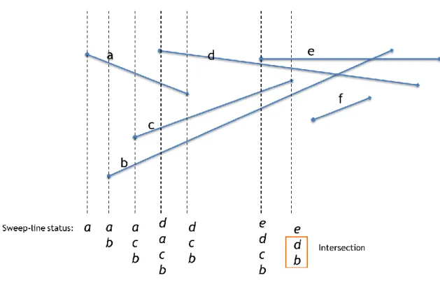
3.5.2 Sweep-line Status
The sweep-line status is updated only at the event points. Figure 3.1 shows the change in sweep-line status at the first seven event points of the six segments. At the event point of type left endpoint, segments are added to the sweep-line status and removed at the event point of type right end-point. When an event point is inserted into the sweep-line status, the segment corresponding to that event
point is checked for intersection with the segments above and below it. With these data structure and their APIs, we can now see the algorithm.
Figure 3.1 Sweep-Line status. Algorithm:
FindIntersections(S)
Input: Set S, of line segments in a plane
Output: The set of intersection points among the segments in S
1. Initialize an empty Event Queue Q
2. Initialize an empty sweep line status data structure
3. Sort the Event points and insert into Q
4. While Q is not empty
5. Determine the next event point p in Q and delete it
6. HandleEventPoint(p)
7. End-While
HandleEventPoint(p)
1. L(p) = segments with left endpoint p
2. R(p) = segments with right endpoint p
3. C(p) = segments with p in interior
4. If |L U R U C| > 1
5. report p as an intersection along with L, R, C
7. T = T – (R U C)
8. T = T U (L U C)
9. If |L U C| = 0
10. let Sb and Sa be the neighbors right below and above p in T
11. FindNewEvent(Sb, Sa, p)
12. Else
13. S = lowest segment in L U C
14. Sb = segment right below S
15. FindNewEvent(Sb, S, p)
16. S = highest segment in L U C
17. Sa = segment right above S
18. FindNewEvent(S, Sa, p)
19. End-If
FindNewEvent(Sl, Sr, p)
1. If Sl and Sr intersect to the right of p
2. Insert the intersection point as an event point in Q
3. End-If
The standard algorithm described here only works for line segments. In order to deal with polylines, we have to modify the FindNewEvent to reject intersections between segments of same polyline.
3.5.3 Finding the intersection point between two segments
Two segments do not intersect if their bounding boxes do not intersect. Checking intersection against bounding boxes enables quick rejections. Sometimes, the bounding boxes might intersect but the segments themselves would not intersect. After checking for bounding box intersection, we have to check if one checking lies entirely on one side of the other segment. This is verified using cross product. Two line segments L1 (P1, P2) and L2 (P3, P4) intersect if and only if each of the two pairs of cross products have different signs or one cross product in the pair is 0.
(P1 - P4) x (P3 - P4) AND (P2 - P4) x (P3 - P4) OR
(P3 - P2) x (P1 - P2) AND (P4 - P2) x (P1 - P2)
After detecting intersection the actual intersection point is obtained through homogenous coordinates method in O(1). The intersection points obtained along with the segments can be used to construct the intersection objects. The type of the intersection can be inferred from the type of the intersecting objects. The implementation details of all the classes are given in Chapter 4.
Before looking at the map software design, we have to choose a suitable application leveraging the data model for conducting the pilot. Participatory GIS field tasks, such as address verification, the process of verifying the master address list and the maps, is where good usability features and
nuances will help the users accomplish the task efficiently. For example, when the user is dealing with handheld devices in the field to do the tasks, the user would benefit from quickly getting information from the map by hovering over the feature or from the various views that we can develop which closely matches the real world perspective and reduce the spatial cognitive processing. These aspects cannot be accomplished by just raster or plain vector data models. With the help of object data model, we can not only accomplish such things but also expand the functionalities by extending the model.
Let’s define the scope and requirements of a map survey experiment which we will use to pilot this software built on the object data model.
3.6 Scope and Requirements of the Map Survey Pilot
In the map survey experiment, the user will use the map software to verify the location of a set of addresses. The user should be able to zoom and pan the map to navigate to the address and perform map-edit functions to correct any errors in the map. Due to the scope of the project, let’s handle correcting the incorrect house locations on the map. This will involve adding or deleting spot objects on the map. During the process, we should be able to obtain the reasons for the edit actions that the user performs on the map. With this on our plate, we have a notion of a user taking part in an experiment which involves taking zero or non-zero edit actions on the map to ‘correct’ it. The following are the requirements for the experiment package design.
1. We will have many users taking part in the experiment 2. An experiment consists are many tasks
3. A user performs an action which has a result i.e., change or no change in the state of the experiment.
4. A task has prescribed action to be taken which will make the result reach the final state. 5. We will be able to query the state of the experiment at any point.
6. Some tasks have 2-step action to be taken, so we will have to maintain the state of the task.
3.7 Specifications for the User Interface
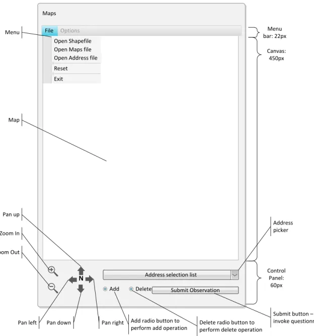
The main UI should have an area to display various options to the users. In order to save space, this should be a menu bar with sub menus. The major portion of the UI should be the area where the map is displayed. There should be a control panel to accommodate interaction controls such as the zoom in, zoom out buttons, the pan left, pan right, pan up, pan down buttons, controls to select the map-edit
functions, a button to submit user action. The map-edit controls and the submit buttons can be displayed when doing specific tasks. Figure 3.2 shows the model of the user interface based on the requirements discussed in this chapter.
Maps File Options
Open Address file Open Shapefile Open Maps file Reset Exit
Submit Observation
Add Delete
Address selection list
Menu bar: 22px Control Panel: 60px Canvas: 450px Zoom In Zoom Out
Pan left Pan down Pan right
Pan up
Delete radio button to perform delete operation Add radio button to
perform add operation
Submit button – to invoke questionnaire Address picker Map Menu N
Figure 3.2 Mockup of the Maps software user interface.
CHAPTER 4. IMPLEMENTATION
This chapter covers the implementation details of the Map software. After consideration between Java and the Dot Net framework, the application was implemented using C# and Windows Presentation Foundation (WPF) which offers powerful functionalities for developing user facing mobile application.
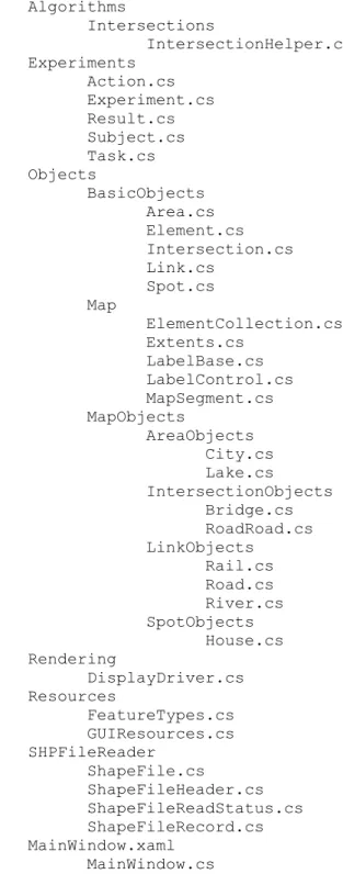
4.1Namespace Structure
The structure of the project is shown in Figure 4.1. The main namespace is the Map, which is shown on top. Within the Map namespace (NS), we have the Algorithms, Experiments, Objects,
Rendering, Resources, SHPFileReader, and Utils namespaces.
NS Algorithms contains the implementation of the algorithms such as the computing intersection.
Experiments NS contains all the classes that represents the experiment, subjects involved in the experiment, tasks that are part of the experiment, actions taken during the experiment and results achieved in the experiment. The Objects NS contains the abstraction about the map features. Within the Objects NS, the BasicObjects NS contains mostly the base classes which represent the very basic features of a digital map. For instance, Element is the base class at the lowest level. Area,
Link, Spot, Intersection are first level derived classes. Map NS contains classes that represent information about the map itself like the extents of the map (Extents.cs), segment of a map (MapSegment.cs). LabelControl represents the on-screen text geometries which are discussed in detail later in this chapter.
MapObjects NS contains all the second level derived classes that are derived from Area,
Intersection, Link and Spot. Rendering NS contains the implementation for constructing and rendering map features on screen. Resources NS was designed to have all the implementation related to describing specifications. Onboarding new features and writing specifications for them is easier in this way. For instance, to add a feature, say Parking, add it to FeatureTypes and defined formatting specifications in GUIResources. SHPFileReader models the shape file and provides APIs for reading it. Utils NS contains code for miscellaneous utility functions. MainWindow is the XAML that contains all the GUI components and their associated Event descriptions.
Map Algorithms Intersections IntersectionHelper.cs Experiments Action.cs Experiment.cs Result.cs Subject.cs Task.cs Objects BasicObjects Area.cs Element.cs Intersection.cs Link.cs Spot.cs Map ElementCollection.cs Extents.cs LabelBase.cs LabelControl.cs MapSegment.cs MapObjects AreaObjects City.cs Lake.cs IntersectionObjects Bridge.cs RoadRoad.cs LinkObjects Rail.cs Road.cs River.cs SpotObjects House.cs Rendering DisplayDriver.cs Resources FeatureTypes.cs GUIResources.cs SHPFileReader ShapeFile.cs ShapeFileHeader.cs ShapeFileReadStatus.cs ShapeFileRecord.cs MainWindow.xaml MainWindow.cs
Figure 4.1 Project Structure.
The rest of the chapter describes the specifications of input data and the process of reading them, constructing map objects, rendering them and implementation of map survey experiment.
4.2Steps Involved: An overview 1. Read the input OMap file
2. Parse all the shape files specified in input file 3. Construct shapes for rendering
4. Construct map objects 5. Load address data file 6. Construct experiment
7. Conduct experiment
4.3Reading the Maps input fil e
All the shapefiles that forms the feature set of a map segment are described in the OMap file. It is an XML file describing the shapefile location in the format given below.
<?xml version="1.0" encoding="UTF-8"?> <fileSet> <shapefile>.//data//AmesCity.shp</shapefile> <shapefile>.//data//AmesMapSpots.shp</shapefile> <shapefile>.//data//AmesRoads.shp</shapefile> <shapefile>.//data//AmesRail.shp</shapefile> <shapefile>.//data//AmesRiver.shp</shapefile> <shapefile>.//data//AmesLake.shp</shapefile> </fileSet>
The naming convention for the shapefile is to have the feature type on the filename. The standard XML reader XmlDocument from the System.Xml namespace is used to parse the OMap file. After getting the list of files to be loaded, each file is checked for existence and then parsed one by one.
4.4Parsing the Shapefiles
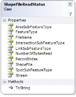
An instance of the class ShapeFileReadStatus stores information about the shapefile being read like filename, feature type and subtype, number of bytes read etc. Figure 4.2 is the class diagram of the ShapeFileReadStatus. The header of the shapefile is read first to find out the filelength, shapetype and the extents of the shapefile. After the header, the shapes are read record after record as a block of 500 shapes and stored in the temporary Collection associated with the
the shape records are parsed, the attribute file is read and stored in the same ShapeFileReadStatus
instance. Once the attribute file is read, the process of constructing map objects and rendering them is started.
Figure 4.2 Class diagram of ShapeFileReadStatus. 4.5Constructing Shape objects
In Chapter 3, the theoretical idea of class design was discussed. When using a framework such as WPF for generating the maps, we can make use of the abstraction provided by the framework itself, i.e., instead of creating classes for representing Point, Line Segment, Label etc., we can make use of
EllipseGeometry, PathGeometry, FormattedText classes available in the standard library. As discussed in Chapter 3, WPF supports Canvas control, on which shapes can be drawn. Shape is an abstract class that represents any draw-able objects such ellipse, polygon, rectangle etc. The shape to be drawn is specified in terms of an instance of type Geometry, such as the one’s stated above. For instance, a line segment is made of two points. This can be represented by the PathFigure class whose Segments property contains the sequence of points that make up the line segment or polyline. The Segments property has Start property which represents the starting point and Next which represents the next sequential point. In order to draw this, we have to use the PathGeometry class and set the Data property of it to this PathFigure which represents a connected curve or a line. So moving from the notion of Point, LineSegment, and Area being the base classes for the geometries that are draw-able, a Shape object will abstract all of them and will be the draw-able entity in this design. The very basic attributes that are common across all the classes such as Shape, Label, and
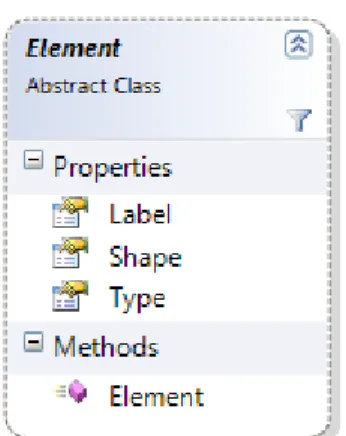
FeatureType are modeled as the abstract class named Element. During the rendering process, the method GetObjectBasedOnType takes in the shapefile record and information about shape, shapetype and returns an instance of type Element which is constructed based on the shapetype. Let’s see the shape and map object construction process in more detail. The class diagram for
Element is given in Figure 4.3.
Figure 4.3 Class diagram of Element.
Similar to the shapefile reading process, the rendering process is also done as a block of 500 objects. As stated earlier, the map object types like River, Street, Lake, etc., are identified using the shapefile’s filename. Based on the map object type, appropriate column information is read from the attributes data associated with the shape being constructed to obtain necessary metadata about the shape. For instance, the attribute database about a House contains a column 'LOTNO' and Street,
River contains a column 'FULLNAME' which is the on screen name for the respective features. Then the actual Shape objects are created based on the shapetype namely Point or MultiPoint, Polygon, or PolyLine. But before that, we have to transform the latitude-longitude coordinates to on screen coordinates to render them correctly. Since we will be dealing with a small portion of the geographical area most of the time, the shapes will be rendered very small on screen, if not scaled properly. In WPF, the Transform class is an abstract class that describes how a coordinate is transformed when it is rendered. For example, a point in the 2-dimensional space can be scaled, moved by an offset in either x or y plane or both or a line segment can be rotated by an angle.
TransformGroup is a Collection of Tranform instances. If the aspect ratio of the shapefile extent is smaller, we have to scale it up or down height wise, i.e., by the ratio of canvas height to extent height and if aspect ratio of the extent is greater, by a ratio of canvas width to extent width. This is achieved by a ScaleTransform. Using a TranslateTransform, the XMin and YMin are
mapped to the origin of canvas. TranslateTransform defines how an object should be moved in a 2-D plane. It is to be noted that the origin of the canvas is in top left. Once the actual screen coordinates are obtained by applying transformation, we can construct the Shape instances.
Point: If the feature is a House, in order to make it more intuitive, the lot number is used to represent the shape on the map. Text can be placed on the canvas as a simple Label instance but it is not that flexible when it comes to formatting. But WPF provides methods to convert text to a Geometry
instance which enables us to add formatting to the text on screen. So for the Point shape type, if the feature is a House, a FormattedText instance is constructed from the lot number along with other specification such as font size, font, and direction of flow. Using the method, BuildGeometry of the same class, a Geometry instance is created to which formatting like color overlay, stroke, images can be added. In order to make the lot number more readable on the map, a RectangleGeometry is added as overlay. For the House object’s shape, this Geometry instance is added to the Canvas later for rendering. For any other Point shape type, an EllipseGeometry instance with equal height and width is created to represent the feature as a Point on the map.
In this version of the software, the Point shapes handled are that of the House objects. Metadata about the house, such as the street name and lot number are stored in the Tag attribute of the Path
instance for later use which is described in the Experiments construction section.
PolyLine or Polygon: PolyLine and Polygon are obtained using the same method of construction except that the start point and last point are the same in case of Polygon. Based on the number of parts information available in the shape record and the number of points within each part, PolyLines are created using the PathFigure class which connects a Collection of points sequentially. So a shape record that has many parts, each containing more than one point would be a Collection of
PathFigure objects. The Collection of PathFigure is abstracted into a single PathGeometry
instance, which is of type Geometry.
After constructing the shapes, formatting is applied to them as appropriate. WPF supports excellent formatting options for basic geometric features like ellipse, lines, curves, polygons. The class
GUIResources acts as a single point of reference for all formatting specifications of the map objects. For instance, for formatting a House object attributes such as, a Color, Stroke color,
StrokeThickness are needed. For formatting a Rail object, in addition to the ones needed for
described in this class. In the future iterations, these formatting specifications can be described in a separate clear text configuration file such as a JSON or XML file.
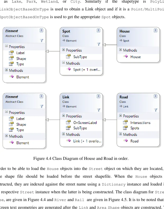
Once the Shape object is created, it is used to construct the map object. If the shapefile type is a polygon, the method GetAreaObjectBasedOnType is called to obtain the map object of type Area
such as Lake, Park, Wetland, or City. Similarly if the shapetype is PolyLine,
GetLinkObjectBasedOnType is used to obtain a Link object and if it is a Point/MultiPoint,
GetSpotObjectBasedOnType is used to get the appropriate Spot objects.
Figure 4.4 Class Diagram of House and Road in order.
In order to be able to load the House objects into the Street object on which they are located, the house shape file should be loaded before the street shapefile. When the House objects are constructed, they are indexed against the street name using a Dictionary instance and loaded into their respective Street instance when the latter is being constructed. The class diagram for Street,
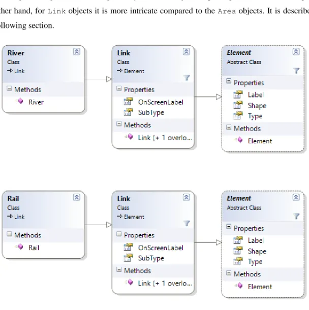
House, are given in Figure 4.4 and River and Rail are given in Figure 4.5. It is to be noted that the on-screen text geometries are generated after the Link and AreaShape objects are constructed. The
process of generating on-screen text geometry for Area objects is placing a Label on the shape. On the other hand, for Link objects it is more intricate compared to the Area objects. It is described in the following section.
Figure 4.5 Class Diagram of River and Rail in order.
4.6Generating On Screen Text for Link Objects
As described in Chapter 3, since most of the map features such as rivers, roads, rails are not always straight lines but “curvy” polylines, placing text along the lines is not straightforward. The position and orientation of each and every character of the label (street name, railroad name) should be calculated with respect to the feature. WPF provides useful APIs to ease our work in implementing these features. The details about the implementation are given below.
4.6.1 Calculating position and orientation
If we were to place characters on a horizontal line segment AB, we can place the first character C1 at Point A and 2nd character C2 at A.X + w, where w equals the width of C1 and A.X is the x coordinate
of Point A, and so on. To calculate the position of a character in the Canvas, we have to know the on-screen width of the character, so each of the character is converted into a TextBlock instance with a font size of 10. TextBlock has a property called DesiredSize which is the size of the
TextBlock. The Width property is obtained from this DesiredSize. Now, we have the starting point of the line and the width of the characters. Since we are not dealing with a horizontal line segment, we need to be able to find points on the line segment to place the characters and the angle to which each of them should be rotated to make them aligned with the line segment. The
PathGeometry class has a method GetPointAtFractionLength which takes fractional length, d, as parameter and gives out a Point on the polyline that is at a distance d from its starting point and a tangent vector at that Point. In order to find the fractional lengths for each character, we maintain a variable progress that tracks the progress on the polyline as we place character one after the other. Since the width of each character is less, we do not essentially pass the progress as such to
GetPointAtFractionLength but with half of the width of the character to be placed.
progress = (progress + width / 2)/ polyLineLength
Since we have supplied a point that is the center of the character’s baseline, we will be rotating the character to the required angle with that point as pivot. Angle is obtained by the following formula with Point T as the tangential vector.
angle = Math.Atan2(T.Y, T.X) * 180 / Math.PI;
The first character was placed at a point at a distance of d from the starting point. Let’s say it was at a fractional length L. Now if we add the half of width of the 2nd character to L and follow the same process, we will get the position and orientation of it. This procedure is done for all the characters keeping track of the fractional length.
After generating the on screen geometry, the map object is fully constructed. After this, the Shape
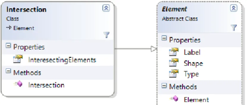
and the on-screen text are added to the Canvas. After loading all the shapes, intersections are computed and Intersection objects are created and rendered. Intersections are computed among the shapes of type Polygon and Polyline. Since we should not compute intersections between the line segments of a Polyline, each Shape when constructed is assigned a unique ShapeID. Intersection objects are not constructed when intersection is detected between line segments with same ShapeID. The intersecting segments are added to a Collection in the Intersection object. The class diagram for the Intersection class is shown in Figure 4.6. In the following section, the implementation details of the user interface controls are described.
Figure 4.6 Class Diagram of Intersection. 4.7User interface Controls:
4.7.1 Zooming and Panning
Zoom control in the main UI is built using standard Button and since arrow shapes are used to display the direction of pan, arrow shapes were drawn on a Canvas control. Mouseover and
MouseDown events are defined on both zoom and pan controls to handle them. When we zoom-in on a shape, we are essentially scaling the shape up and vice versa. In order to achieve this we use the
ScaleTransform class of the transformation library available in WPF. The construction of the
ScaleTransform object is given below.
ScaleTransform zoomTransform = new ScaleTransform();
When we are panning, we are moving the origin by some offset, either in upward, downward or left or right direction. The TranslateTransform class supports translating the coordinates of the shape. A sample declaration is given below.
TranslateTransform panTransform = new TranslateTransform();
We can use the TransformGroup class to group the Transform objects together such as the
ScaleTransform and TranslateTransform.
TransformGroup viewTransform = new TransformGroup(); this.viewTransform.Children.Add(zoomTransform); this.viewTransform.Children.Add(panTransform);
This TransformGroup object can be attached to the geometries transformation properties on screen so that shape transformations are reflected on the geometries when the transformation properties change.
For instance,
GeometryGroup geometry = new GeometryGroup(); geometry = ConstructGeometry(); geometry.Transform = this.viewTransform;
The ScaleTransform object is supplied with appropriate value to scale the objects it is associated to.
this.zoomTransform.ScaleX = zoomFactor; this.zoomTransform.ScaleY = zoomFactor;
Similarly, the TranslateTransform object is supplied with an offset value to get the shapes on the canvas transformed.
this.panTransform.X += xOffset; this.panTransform.Y += yOffset;
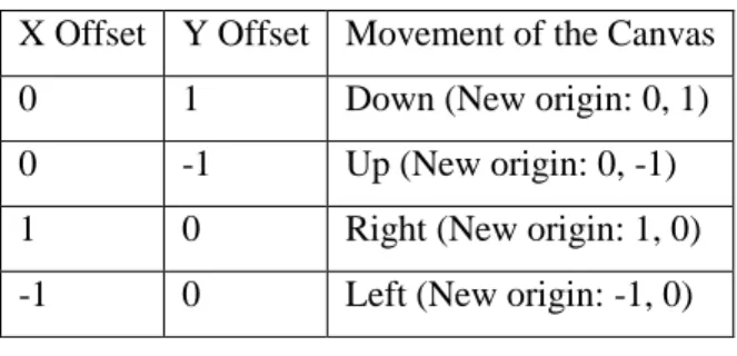
Table 4.1 shows the transformation offsets for the pan movements. Table 4.1 Pan movement of the Canvas. X Offset Y Offset Movement of the Canvas
0 1 Down (New origin: 0, 1)
0 -1 Up (New origin: 0, -1)
1 0 Right (New origin: 1, 0)
-1 0 Left (New origin: -1, 0)
It should be noted that the origin of the Canvas is at the top left.
4.7.2 Hovering
It will be useful to get information about the map features just by hovering over the feature. The
ToolTip property of the map features is set to appropriate value to display information to the user on hovering. E.g., street names for streets, lot numbers for houses, intersecting streets for intersections. The next section describes the Experiments namespace and its classes.
4.8Handling Address Canvasing Task with Object Maps Software
4.8.1 Loading the Address Verification data
The address data file is an XML file with a format given below. The addressSet tag is the root node which consists of all the addresses as children. The address tag specifies the individual address and the task, i.e., the status of the task to be performed. The various tasks that can be performed and their values are explained in detail in Chapter 5.
<addressSet> <address>
<lot>2103</lot>
<street>Country Club Blvd</street> <city>Ames</city> <county>Story</county> <state>Iowa</state> <zip>50011</zip> <task>wrongposition</task> </address> <addressSet>
The address data file is parsed with a standard XML parser and the addresses used in the experiment are highlighted by changing the Color of the Shape. This is possible because, the streets are indexed using the street name and houses are indexed using the lot number and street name at the time of their construction. A Dictionary instance is used for indexing to get reference to the Shape objects in O(1). The addresses used in the experiment are displayed in the main UI using a standard ComboBox
control. OnClick and OnValueChanged events are registered to the ComboBox items in order to respond to various user actions such as selecting an address.
4.8.2 Constructing an Experiment
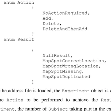
A separate namespace was designed to conduct the experiment and maintain the state of the experiment as per the requirements described in Chapter 3. Since Result and Action detailed in the use cases just takes different states, we can use Enum to model the various values it takes. The definition of the Result and Actionenums are given below.
enum Action { NoActionRequired, Add, Delete, DeleteAndThenAdd } enum Result { NullResult, MapSpotCorrectLocation, MapSpotWrongLocation, MapSpotMissing, MapSpotDuplicated }
When the address file is loaded, the Experiment object is constructed. It contains the List of Task
and the Action to be performed to achieve the Result that marks the completion of the
Experiment, the number of Subject taking part in the experiment, the state of the current Subject taking part in the experiment. Let’s get into the details of the implementation.
Once the address data file is parsed, the List of the address and the type of the task to be performed is passed to a static GetNewExperiment method. Based on the task, appropriate Result variable is created and passed to the Task constructed along with the address. In the constructor, the status variables and the final variable that represents the action to be taken are initialized based on the end result, summarized in the below table. It is to be noted that the Result.NullResult represents value for user clicking on the submit button without any action. The status variables represent the state of the action taken and booleanAND of them gives the status of the completion of the Task.
Table 4.2 Result, Action, Status map.
Result Action to be taken Add Status Delete Status Result.MapSpotCorrectLocation Action.NoActionRequired TRUE TRUE
Result.MapSpotDuplicated Action.Delete TRUE FALSE
Result.MapSpotMissing Action.Add FALSE TRUE
Result.MapSpotWrongLocation Action.DeleteAndThenAdd FALSE FALSE
The address string is also saved as part of the state variable of the Task object, so that we can later verify, when conducting the experiment, if the address the user picked on the map and the task address at hand matches. The GetNewExperiment method takes in the number of subjects to be constructed as an argument and along with the List of Task objects just constructed; the Subject
objects are constructed and given a unique SubjectID. The mapping of the street address to the
Task is maintained using a Dictionary object which is shown below.
Dictionary<string, Task> taskMap;
The status of Task can be obtained by AND-ing add and delete status variable as discussed in Table 4.2. This enables us to quickly query and check the status of the task when the user performs action on the map so that invalid actions can be discarded without further processing. Since the status of each Task is preserved, a user can switch between tasks easily. After the Subject objects are initialized, the Experiment object is fully constructed and the experiment is ready to begin.
4.8.3 Experiment Controls
At the bottom of the main window, there are two Radio Button, add and delete which are used to add and delete the map spots respectively. The Submit Observation Button is used for invoking the questionnaire screen for submitting the user observation about the task in hand. In the questionnaire screen, a TextBlock control displays a question and four Radio Button control displays the list of choices. Once the user clicks and submits the right answer to the questionnaire, Exit to Map Button
appears to enable the user to go to the main map screen.
4.8.4 Experiment procedure
The flow of the experiment procedure is show in Figure 4.7. As shown in the flow diagram, the user is allowed to select any task from the drop down menu. Once the user selects an address, the
OnSelectionChanged event is triggered. At this point, we check if the status of the task the user has just selected is incomplete. If it is,, then we change the value of the current task at hand and automatically pan the map to show the street selected. When the user is ready to enter the information about the observation made from the real world, the user clicks on the Submit Observation Button. The Click event is triggered and the questionnaire screen is invoked, in which the user clicks on the choice that matches his observation. If the user has chosen the right choice, the user is presented with instructions to complete the task. For instance, for a task involving adding a missing spot, the user is asked to exit the questionnaire screen, click on the add option and then click on the correct spot where the map spot needs to be added. This is accomplished by the API provided by the Task class to verify the answer. When user submits the answers to the questionnaire, the SubmitAnswer method in the
Subject class is invoked which submits the Result the user has chosen to the IsAnswerCorrect
method in the Task class, which returns TRUE if the user input the correct observation in the questionnaire or FALSE if otherwise. In the answer is correct, Proceed to Action Button appears, if
incorrect, Exit to Map Button appears, both for the user to be able to exit the questionnaire screen and proceed to next step.
Start
Pick an incomplete task
Make observation from real world and Submit
Is observation correct?
Perform Map-edit functions
Are all tasks completed? End Yes Yes No No
Figure 4.7 Map Survey Experiment Flow Diagram.
After getting the choice right in the questionnaire, the user should complete the map-edit task. The user specifies his intention to add or delete a map spot by clicking on the Add or Delete Radio Button. If the task at hand is to delete an incorrect map spot, the user can only delete the designated map spot for that task. This is done by validating the picked map spot against that of the address in the task at hand. It is to be noted that we stored the metadata about the map spot in the Tag property of the map spot Shape. Since the map spots are indexed by their address, querying is done quickly. If the user picked the right map spot, we essentially hide the spot from the map, otherwise we perform a
user tries to add a spot (if the task requires such an action). On the other hand, if the task is to add a spot, the user is allowed to place it anywhere. When the user clicks on the map, a spot with the right lot number appears on the map. As stated earlier, a hidden spot is repositioned and shown. Hiding and un-hiding is accomplished by setting the Visibility property to Collapsed and Visible
respectively. The position for placing the map spot in the new location is obtained from the mouse position when MouseDown event is triggered by clicking on the map. When all the tasks are complete, the experiment is marked as completed, and the user is not allowed to take any map-edit actions on the map.
The next chapter discusses the experiment conducted, experiences gained, and feedbacks obtained from the participants.
CHAPTER 5.
PILOT
This chapter details the methods and procedure used in conducting the pilot to evaluate the effectiveness of the data model and maps software and the observations on user interaction behavior during the pilot.
5.1 Participants, Task, Environment and Expectation
Five participants who are students of Iowa State University were selected for the pilot with varied computer experience. The participants were asked to perform the address verification task which involves interacting with the map to navigate from one place to another. Precisely, the participants were asked to verify the correctness of house numbers on the map. The map spot that describes a house on a street can satisfy any one of the following condition.
1. House spot is in the correct location
2. House spot is in the incorrect location on the map 3. House spot appears twice on the same street 4. House spot is missing on the map
The participants were provided with 6 different addresses to verify which involves navigating through complex road intersections. Figure 5.1 shows the change log of the 6 addresses on the map which the participants will revert to the correct condition. The participants were given a tablet computer loaded with the Map software to accomplish the tasks. Prior to this exercise, the participants were provided training in completing the address verification task using the Map software. The features of the Map software that would help the participants complete the tasks were outlined and they were allowed to get the doubts clarified before starting the actual exercise.
The pilot was conducted in the virtual reality (VR) environment called the C6 located in Virtual Reality Application Center at Iowa State University. The VR model used was designed to be a replica of a real world neighborhood in Ames where the training and exercise addresses are located. The map region is show in Figure 5.1 with the changes and the changes are shown in table 5.1. The VR model was developed by Kofi Whitney and Adam Van Gorp.
The participants were also trained on using and navigating through the streets of the VR environment. During the pilot, the participants’ behavior and their interaction with Map software were observed.
Table 5.1 Summary of changes made to the map
S No Address Change
1
2103 Country
club Moved from east on Country Club to north on Country Club (see arrow)
2
2110 Country club
Added to the map, users have to delete it. Here, we would have two 2110 addresses, one on each side of Country club (see red dot)
3 2111 Graeber Moved to south side of Graeber 4 2030 Cessna Moved to north of Cessna 5 2124 Hughes Moved to east side of Hughes
6 2116 Cessna Deleted from the map, users have to add it
A survey questionnaire was developed for the participants to rate the various aspects of the map software which is given in Appendix A. First, the activities observed during the pilot are discussed. The expected outcome of the pilot was to obtain patterns in user interaction behavior, effects of the data model of maps in improving the usability of the map software and identify any areas of future improvements.
5.2Observations
5.2.1 Task Execution
1 out of the 5 participants planned their route upfront before starting each task. About 4 out of the 5 participants had the natural tendency to select the next item from the randomized address list rather than the one closest to their current position. All the participants did not make any mistakes when correcting the addresses. Four out of the 5 users interacted with the map at maximum zoom level.
5.2.2 Spatial Ability
Though the street pertaining to the current address being verified was highlighted with a different color, 4 out of the 5 participants were, at least once, pointing to the same house number from another street other than the one they were currently in. All the participants tried to orient themselves to the map by turning the tablet. Though indicated in the training about the zoom and pan controls, about 2 out of the 5 participants tried to zoom and pan using multi-gesture touch input instead of button based input. All the users retraced their path backward and went forward to make sure they were in the correct location corresponding to the current address in the task. Only 1 out of the 5 participants made
efforts to place the map-spot in a location which was close to the actual location. All the participants visited one side of the street and back traced the path and visited the other side of the street.
5.2.3 Training
Though indicated during the training session and the screen via instructions, during the exercise, 2 out of the 5 participants were confused about the sequence of operation required to complete the task.
5.2.4 Map Interactions
Another important thing noted was, when the participants interacted with the touch based device, they were often pointing at positions near the map controls which made them tap on the screen multiple times. They assumed that the software was not responding.
5.2.5 Map Features
The auto-zoom feature seemed to dislocate the participants spatially as they had to plan their route to the next task seeing the map which negatively impacted their performance in terms of number of map interaction required for them to complete the task correctly. Highlighting the streets where addresses had to be verified positively impacted as they quickly took directions in the VR world based on the streets displayed in the Map software and the VR.
Twenty percent of the participants used the feature tips to help them take the right direction at the intersections. The position of the street names on the street appeared to be important for the users to locate themselves spatially. When the street name was not visible in the visible map part, the participants had to either zoom out and zoom in again to identify themselves spatially or had to pan back and forth in either north-south direction or west-east direction.
In the following section, participant’s response to the questionnaire is discussed. 5.3 Results of the questionnaire
Figure 5.2 gives the summary of responses to the questionnaire obtained post-pilot from the participants.
Figure 5.2 Summary of participant’s responses.
Table 5.2 summarizes the average score of the usability items based on the participant’s responses Table 5.2 Score range of the questionnaire items.
Item Score Range
Highlighting streets simplifies task 5 to 9
Sequence of screens 6 to 9
Reading characters on the screen 7 to 9 Position of messages on screen 6 to 9 Learning to use the map software 7 to 9 Performing tasks is straightforward 5 to 9 Instructions on the screen 4 to 9 Interacting with the map (zoom, pan) 0 to 9 Information on street location,
intersections helped navigating? 3 to 9 Information on next step of the task 5 to 9
Correcting mistakes 6 to 9
The next chapter details the conclusions derived and future directions. 0 1 2 3 4 5 6 7 8 9 10 P 1 P 2 P 3 P 4 P 5
CHAPTER 6. SUMMARY AND FUTURE DIRECTIONS
In this chapter we will summarize our work and some of future directions.
6.1Summary
Through this work, we have developed a data model that represents geographic data on an application level which can be easily integrated and extended for further studies. We discussed the design of the classes representing common map features using object oriented principles. We also discussed methods to computationally determine secondary features such as intersections.
The object model used vector format as underlying data which is the right choice for manipulating and developing various usability features. The data model provides us with the flexibility to extend it and onboard more and more metadata about the map feature so as to make the applications built on top of it resourceful. This helps deliver sophisticated GIS capabilities to field work where computing power and storage is less and network connectivity is mostly absent.
We developed maps software using this model which enabled the user to interact with the maps by zooming, panning, navigating and editing the map features. A pilot was conducted in a virtual reality environment to study the usability of the software and the results and experiences gave us ideas on future directions which are discussed below.
6.2 Future Di