Nonparametric Predictive Inference for Multiple Comparisons

(1)

Durham E-Theses

Nonparametric Predictive Inference for Multiple

Comparisons

MATURI, TAHANI

How to cite:

MATURI, TAHANI (2010) Nonparametric Predictive Inference for Multiple Comparisons, Durham theses, Durham University. Available at Durham E-Theses Online: http://etheses.dur.ac.uk/230/

Use policy

The full-text may be used and/or reproduced, and given to third parties in any format or medium, without prior permission or charge, for personal research or study, educational, or not-for-prot purposes provided that:

• a full bibliographic reference is made to the original source • alinkis made to the metadata record in Durham E-Theses • the full-text is not changed in any way

The full-text must not be sold in any format or medium without the formal permission of the copyright holders. Please consult thefull Durham E-Theses policyfor further details.

Academic Support Oce, Durham University, University Oce, Old Elvet, Durham DH1 3HP e-mail: [email protected] Tel: +44 0191 334 6107

(2)

Nonparametric Predictive Inference

for Multiple Comparisons

Tahani A. Maturi

A thesis presented for the degree of

Doctor of Philosophy

Department of Mathematical Sciences

Durham University

UK

May 2010

(3)

Dedicated

(4)

Nonparametric Predictive Inference for Multiple

Comparisons

Tahani A. Maturi

Submitted for the degree of Doctor of Philosophy

May 2010

Abstract

This thesis presents Nonparametric Predictive Inference (NPI) for several multiple comparisons problems. We introduce NPI for comparison of multiple groups of data including right-censored observations. Different right-censoring schemes discussed are early termination of an experiment, progressive censoring and competing risks. Several selection events of interest are considered including selecting the best group, the subset of best groups, and the subset including the best group. The proposed methods use lower and upper probabilities for some events of interest formulated in terms of the next future observation per group. For each of these problems the required assumptions are Hill’s assumption A(n) and the generalized assumption rc-A(n) for right-censored data.

Attention is also given to the situation where only a part of the data range is considered relevant for the inference, where in addition the numbers of observations to the left and to the right of this range are known. Throughout this thesis, our methods are illustrated and discussed via examples with data from the literature.

(5)

Declaration

The work in this thesis is based on research carried out at the Department of Mathe-matical Sciences, Durham University, UK. No part of this thesis has been submitted elsewhere for any other degree or qualification and it is all the author’s original work unless referenced to the contrary in the text.

Copyright c 2010 by Tahani A. Maturi.

The copyright of this thesis rests with the author. No quotations from it should be published without the author’s prior written consent and information derived from it should be acknowledged.

(6)

Acknowledgements

My main appreciation and thanks go to my first supervisor Dr. Pauline Coolen-Schrijner. To my great sadness, Pauline passed away on 23 April 2008 due to her illness. She was a very supportive and nice person, who helped me greatly during my study, which will have significant impact on my future career. I hope she is proud of this thesis.

My special thanks go to my second supervisor Prof. Frank Coolen for his unlim-ited support, expert advice and guidance.

Mathematics is not a subject to me; it is my love in life. This is because of my lovely mother who taught me mathematics from an early age when mathematics was my reward for learning the alphabet. Without my mother and her prayer I would not be at this stage of my career in mathematics.

I am immensely grateful to my parents, my brothers (especially Hani who came along with me to the UK), my lovely sister Amani and my dearest cousin Dalal for their invaluable care, support and encouragement.

My final thanks go to King Abdulaziz University, Jeddah, Saudi Arabia, for offering me the opportunity to complete my studies abroad.

(7)

Chapter 1

Introduction

1.1

Overview

This thesis presents Nonparametric Predictive Inference (NPI) for several compar-isons problems. Mainly, we introduce NPI for multiple comparcompar-isons in situations with right-censored observations. Such data typically occur in reliability or survival analysis, due to several reasons. For example, when interest is in a specific failure mode for a technical unit, it may fail due to a different failure cause. If multiple failure modes are of interest, and failure will be due to only a single failure mode, then this situation is known as ’competing risks’, where an observed failure time is actually a right-censoring time with regard to all failure modes that did not cause the failure. Another reason for right-censoring may be removal of units from a life-time experiment, normally to save life-time or reduce costs, but this also occurs if, at some point, one wishes to study in more detail units which have not yet failed in an experiment. If right-censoring is due to an experiment being terminated before all units have failed, comparison of different groups of units based on such data is known as ’precedence testing’. If non-failing units are removed from the experiment at several possible stages it is known as ’progressive censoring’.

In this thesis, we develop NPI for multiple comparisons for precedence testing, progressive censoring, and competing risks. It should be emphasized that, through-out the thesis, unspecified reasons for right-censoring are assumed to be based on processes that are independent of the residual lifetimes of the censored units. We

(11)

1.2. Assumption A(n) and imprecise probability 2 also present NPI for situations where the information available consists of precise measurements of real-valued data only within a specific range, with in addition the numbers of observations to the left and to the right of this range are known.

Section 1.2 provides a brief overview of some basic aspects of imprecise probabil-ity and the underlying assumption behind NPI, Hill’s assumption A(n). In Section 1.3 we review briefly the main idea of NPI and discuss some applications which we will refer to later in the thesis. This includes the generalisation of the A(n) as-sumption needed to accommodate lifetime data, the so-called asas-sumption rc-A(n). Finally, the outline of this thesis is given in Section 1.4.

1.2

Assumption

A

₍_n₎

and imprecise probability

In this section we briefly overview some basic aspects of imprecise probability and the underlying assumption behind NPI, Hill’s assumption A(n) [40]. To introduce

A(n) we first need to introduce some notation. Suppose that X1, . . . , Xn, Xn+1 are real-valued absolutely continuous and exchangeable random quantities. Let the ordered observed values of X1, X2, . . . , Xn be denoted by x1 < x2 < . . . < xn, and

let x0 = −∞ and xn+1 = ∞ for ease of notation. We assume that no ties occur, the results can be generalised to allow ties [42], see also Subsection 1.3.5. Based onn observations, the assumptionA(n) is that the probability that the next future observation Xn+1 falls in the open interval Ij = (xj, xj+1) is 1/(n+ 1), for each

j = 0,1, . . . , n [40].

A(n) does not assume anything else, and can be considered to be a post-data assumption related to exchangeability [31]. Hill [41] discusses A(n) in detail. A(n) is not sufficient to derive precise probabilities for many events of interest, but it provides bounds for probabilities via the ‘fundamental theorem of probability’ [31], which are lower and upper probabilities in interval probability theory [76, 79].

Lower and upper probabilities generalise classical probabilities, and a lower (up-per) probability for eventA, denoted byP(A) (P(A)), can be interpreted in several ways [21]: as supremum buying (infimum selling) price for a gamble on the event

(12)

1.3. Nonparametric Predictive Inference (NPI) 3

follows from the assumptions made. Informally,P(A) (P(A)) can be considered to reflect the evidence in favour of (against) event A.

Interval probabilities, also know as imprecise probabilities, have been suggested in various areas of statistics. Recently increasing attention has been given to this topic area resulting in a series of conferences and a project website (The Society for Imprecise Probability: Theories and Applications - www.sipta.org). Walley [76, 77] extended the traditional subjective probability theory via buying and selling prices for gambles, whereas Weichselberger [78, 79] generalised Kolmogorov’s axioms without imposing an interpretation.

Below we briefly present some elements of theory of interval probability as rele-vant toA(n)-based inference. According to Weichselberger [78, 79], an axiomization of interval probability can be achieved by supplementing Kolmogorov’s axioms as follows:

For a measurable space (Ω,_A), a set functionp(.) on_A satisfying Kolmogorov’s axioms is called a classical probability. Let K(Ω,A) be the set of all classical prob-abilities on (Ω,_A). A function [P(.);P(.)] on _A is called an F-probability with structure M, if

i) P :_{A → {}[P;P]_|0_≤P _≤P _≤1_} and A_7→[P(A);P(A)],

ii) _M:=_{p(.)_{∈ K}(Ω,_A)_|P(A)_≤p(A)_≤P(A),_∀A_{∈ A} 6}=_∅,

iii) For all A_{∈ A}, inf

p(.)∈M p(A) = P(A) and _p₍sup_.₎_∈M p(A) =P(A).

For every F-probability, P(A) and P(A) are conjugated, i.e. P(A) = 1−P(Ac_),

whereAc _{is the complement of} _A_.

1.3

Nonparametric Predictive Inference (NPI)

Inferences based on A(n) are predictive and nonparametric, and can be considered suitable if there is hardly any knowledge about the random quantity of interest, other than the n observations, or if one does not want to use such information, e.g. to study effects of additional assumptions underlying other statistical methods. Nonparametric Predictive Inference (NPI) is a statistical method based on Hill’s

(13)

assumptionA(n) [40], which gives direct probabilities for a future observable random quantity, given observed values of related random quantities [1, 21]. NPI has been developed in recent years, mainly by Frank Coolen and Pauline Coolen-Schrijner and their collaborators and students, for different applications in statistics, reliability and operational research.

In NPI uncertainty is quantified by lower and upper probabilities for events of in-terest. Augustin and Coolen [1] introduced predictive lower and upper probabilities based on A(n) as follows:

Let B be the Borel σ-field over R. For any element B ∈ B, lower probability

P(.) and upper probability P(.) for the event Xn+1 ∈ B, based on the intervals

Ij = (xj, xj+1) (j = 0,1, . . . , n) created by n real-valued non-tied observations, and the assumption A(n), are

P(Xn+1 ∈B) = 1 n+ 1|{j :Ij ⊆B}| P(Xn+1 ∈B) = 1 n+ 1|{j :Ij∩B 6=∅}|

where |A| is the cardinality of a set A, i.e. the number of elements contained in A. In other words, the lower probabilityP(Xn+1 ∈B) is achieved by taking only prob-ability mass into account that is necessarily withinB, which is only the case for the probability mass 1

n+1 per intervalIj if this interval is completely contained withinB. The upper probability P(Xn+1 ∈B) is achieved by taking all the probability mass into account that could possibly be withinB, which is the case for the probability mass _n₊₁1 , per interval Ij, if the intersection of Ij and B is non-empty.

Augustin and Coolen [1] showed that these bounds fit nicely into the framework of interval probability [78, 79]. They proved that, without adding any further as-sumptions, these A(n)-based lower and upper probabilities are F-probability with structure

M:=_{p(.)_{∈ K}(R,_B)_|p(Xn+1 ∈Ij) =

1

n+ 1,∀j = 0,1, . . . , n}.

By the nature of A(n), NPI is a frequentist statistical methodology [1, 40, 41], which however can be interpreted in a way similar to Bayesian statistics [21, 42]. An important advantage over more established frequentist methods is that NPI does

(14)

not depend on counterfactuals, that is data which were not actually observed but could have been observed. For example, these are important in hypothesis testing, which has led to a large literature on frequentist methods for related problems con-sidering slightly varying experimental procedures. In NPI, as in Bayesian statistics, the inferences only involve the actual data observed, although a warning is needed about the fact that, quite obviously, to apply NPI one must be happy with the exchangeability assumption on the data and future observation(s), which may be non-trivial depending on the experimental set-up.

1.3.1

NPI for multiple comparisons

For complete data, Coolen [19] introduced NPI for comparing two independent groups, sayX and Y. In classical statistics these tend to be referred to as ’popula-tions’. Throughout this thesis, we avoid the term ‘populations’ in NPI as we only consider one future observation and do not make use of any population distribution, even no assumptions about existence of such a distribution or about a meaningful population are made. Suppose that X1, . . . , Xnx, Xnx+1 and Y1, . . . , Yny, Yny+1 are real-valued absolutely continuous and exchangeable random quantities fromX and

Y, respectively. Let their ordered observed values be x1 < x2 < . . . < xnx and

y1 < y2 < . . . < yny, and let x0 = y0 = −∞ and xnx+1 = yny+1 = ∞. Again we assume that no ties occur, the results can be generalised to allow ties [42].

Such comparisons focus on the next future observation from each group. The NPI lower and upper probabilities for the event that a future observation,Xnx+1, of group X is less than a future observation, Yny+1, of group Y (i.e. Xnx+1 < Yny+1), based onnx and ny observations of group X and Y, and the assumptions A(nx) for

Xnx+1 and A(ny) for Yny+1, are

P(Xnx+1 < Yny+1) = 1 (nx+ 1)(ny + 1) ny X j=1 nx X i=1 1{xi < yj} (1.1) P(Xnx+1 < Yny+1) = 1 (nx+ 1)(ny + 1) ( ny X j=1 nx X i=1 1{xi < yj}+nx+ny + 1 ) (1.2) where1_{E_}is an indicator function which is equal to 1 if eventE occurs and 0 else. For these lower and upper probabilities the conjugacy property holds, that is for an

(15)

event E and its complementary event Ec_, _P₍_E_{) = 1}₋_P₍_Ec_).

Throughout we assume that information on units from one group does not hold any information about units from the other group, soXnx+1 and Yny+1 are indepen-dent and data from group X contain no information on Yny+1 and vice versa. We call this ‘complete independence’ of the groups.

Coolen and van der Laan [25] extended this to compare k _≥ 2 groups with

different events of interest including selection of the best group, the subset of best groups, and the subset that includes the best group.

Suppose we have k ≥ 2 groups and nj + 1 random quantities from group j,

denoted by Xj,ij where ij = 1,2, . . . , nj, nj + 1, j = 1,2, . . . , k, and let for each groupj (j = 1,2, . . . , k)xj,1 < xj,2 < . . . < xj,nj be the ordered observed values and

xj,0 =−∞ and xj,nj+1 =∞. The inference depends on Hill’s assumption A(nj) [40] for each group j, as described before.

Coolen and van der Laan [25] presented the following NPI lower and upper prob-abilities for the event that a specificXl,nl+1 is the maximum for all next observations

Xj,nj+1, j = 1, . . . , k. P Xl,nl+1 = max 1≤j≤kXj,nj+1 = _k 1 Q j=1 (nj + 1)     nl X il=1 k Y j=1 j6=l nj X ij=1 1{xj,ij < xl,il}     P Xl,nl+1 = max 1≤j≤kXj,nj+1 = _k 1 Q j=1 (nj + 1)     nl X il=1 k Y j=1 j6=l  1 + nj X ij=1 1{xj,ij< xl,il}       + 1 nl+ 1

They also considered selection of a subset of groups such that all the groups in this subset are ’better’ than all not selected groups, that is the next observation of each group in the subset is greater than the next observation of all groups not in the subset. Let S = {l1, l2, ..., lm} be a subset of m groups (1 ≤ m ≤ k −1)

fromk independent groups and let N S be the complement set of S containing the remainingk−m groups. Then the NPI lower and upper probabilities for the event that the next observation of each group inS is greater than the next observation of

(16)

each group inN S, i.e. min

l∈S Xl,nl+1 >jmax∈N SXj,nj+1, are [25] P min l∈S Xl,nl+1 >jmax∈N SXj,nj+1 = _k 1 Q j=1 (nj + 1) nl X XX XXX il=1 l∈S Y j∈N S   nj X ij=1 1{xj,ij <min l∈S{xl,il}}   P min l∈S Xl,nl+1 >jmax∈N SXj,nj+1 = 1 k Q j=1 (nj + 1) nl+1 X XX XXX il=1 l∈S Y j∈N S  1+ nj X ij=1 1{xj,ij<min l∈S{xl,il}}  

where the notation

bl X XX XXX il=a l∈S

is used for the m sums

bl₁ X il₁=a ... b_lm X i_lm=a .

Using the same definitions of subsets S and N S, we can also be interested in selecting the subsetS that contains the best group. Then the NPI lower and upper probabilities for the event that the next observation from (at least) one of the se-lected groups inS is greater than the next observation from each group inN S, i.e. max l∈S Xl,nl+1 >jmax∈N SXj,nj+1, are [25] P max l∈S Xl,nl+1 >maxj∈N SXj,nj+1 = _k 1 Q j=1 (nj+ 1) nl XXXXXX il=0 l∈S Y j∈N S   nj X ij=1 1{xj,ij <max l∈S {xl,il}}   P max l∈S Xl,nl+1 >maxj∈N SXj,nj+1 = 1 k Q j=1 (nj+ 1) nl+1 XXXXXX il=1 l∈S Y j∈N S  1+ nj X ij=1 1_{xj,ij<max l∈S {xl,il}}  

1.3.2

NPI for right-censored data

In reliability and survival analysis, data on event times, often called lifetime, are often affected by right-censoring, where for a specific unit or individual it is only known that the event has not yet taken place at a specific time. An observation for a unit or an individual is said to be right-censored atc when its lifetime is only known to be greater thanc[48].

The assumptionA(n) requires fully observed data, and cannot deal directly with right-censored data. Coolen and Yan [27] presented a generalisation of A(n), called right-censoringA(n) or rc-A(n), which is suitable for right-censored data. In compar-ison to A(n), rc-A(n) uses the extra assumption that, at the moment of censoring,

(17)

the residual lifetime of a right-censored unit is exchangeable with the residual life-times of all other units that have not yet failed or been censored. Further details of rc-A(n) are given in [27]. To formulate the required form of rc-A(n), we need no-tation for probability mass assigned to intervals without further restrictions on the spread within the intervals. Such a partial specification of a probability distribution is called anM-function [27] which is given by the following definition.

Definition 1.1. A partial specification of a probability distribution for a real-valued random quantity X can be provided via probability masses assigned to intervals, without any further restriction on the spread of the probability mass within each interval. A probability mass assigned, in such a way, to an interval (a, b) is denoted byMX(a, b), and referred to as M-function value for X on (a, b).

Clearly, each M-function value should be in [0,1] and all M-function values for

X on all intervals should sum up to one. The concept of M-function is similar to that of Shafer’s ‘basic probability assignment’ [72].

Let X1, . . . , Xn, Xn+1 be positive, continuous and exchangeable random quan-tities representing lifetimes. Suppose that there are n observations of group X

consisting of u event times, x1 < x2 < . . . < xu, and υ(= n−u) right-censored

observations, c1 < c2 < . . . < cυ. Let x0 = 0 and xu+1 = ∞. Suppose further that there are si right-censored observations in the interval (xi, xi+1), denoted by

ci

1 < ci2 < . . . < cisi, so Pu

i=0si = υ. The assumption rc-A(n) partially specifies the NPI-based probability distribution forXn+1 by the followingM-function values, where the random quantityXn+1 represents the failure time of one future unit [27].

Definition 1.2. Right-censoring A(n) (rc-A(n)) partially specifies the probability distribution for the next observationXn+1 by the following M-function values,

M_iX =MXn+1(xi, xi+1) = 1 n+ 1 Y {r:cr<xi} ˜ ncr + 1 ˜ ncr , (1.3) M_i,iX∗ =MXn+1(c i i∗, xi+1) = 1 (n+ 1)˜nci i∗ Y {r:cr<ci_i∗} ˜ ncr + 1 ˜ ncr , (1.4) wherei= 0,1, . . . , u and i∗ _{= 1}_,₂_{, . . . , s} i.

(18)

These M-function values can also be written as (for i = 0,1, . . . , u and i∗ ₌

0,1, . . . , si) MXn+1(t i i∗, xi+1) = 1 n+ 1(˜ntii∗) δi i∗−1 Y {r:cr<ti_i∗} ˜ ncr + 1 ˜ ncr (1.5) where δii∗ =    1 ifi∗ _{= 0} _i.e. _ti

0 =xi (failure time or time 0)

0 ifi∗ _{= 1}_{, . . . , s}

i i.e. tii∗ =ci_i∗ (censoring time)

and ñcr and ñti_i∗ are the numbers of units in the risk sets (still functioning or alive and uncensored) just prior to time cr and tii∗, respectively. For consistency of notation, the further definition ñ0 = n + 1 is used throughout. Only intervals of this form have positive M-function values, and these sum up to one over all these intervals. Summing up all M-function values assigned to such intervals with the same xi+1 as right end point gives the probability

Pi =P(Xn+1 ∈(xi, xi+1)) = 1 n+ 1 Y {r:cr<xi+1} ˜ ncr + 1 ˜ ncr (1.6)

where xi and xi+1 are two sequential failure times (and x0 = 0, xu+1 = ∞). It should be noted that, throughout this thesis, the product taken over an empty set is defined to be equal to one. To get more insight in rc-A(n), we provide an illustrative example in Appendix A.

Below two useful equalities are given which will be used later in the thesis, these were presented and proven in [27, p. 51].

Lemma 1.1. The following two equalities hold, for all i= 0,1, . . . , u, (a) si X i∗₌₂ 1 ˜ nci i∗n˜c i i∗−1 = 1 ˜ nci si − 1 ˜ nci 1 for si ≥2 (b) 1 + si X i∗₌₁ 1 ˜ nci i∗ Y {r:xi<cr<ci_i∗} ˜ ncr + 1 ˜ ncr = Y {r:xi<cr<xi+1} ˜ ncr + 1 ˜ ncr for si ≥1.

(19)

1.3.3

NPI for survival function

A commonly used method for summarizing lifetime data is the survival function,

S(t), which specifies the probability that the time to event is greater than t. In a sample of size n, suppose that there are q (q _≤ n) distinct event times x1 < x2 <

· · ·< xq. Let hi be the number of events that occur at time xi, and ˜nxi the number of units in the risk set just prior to time xi. The product-limit estimator of the

survival function, first proposed by Kaplan and Meier (KM) [44], is ˆ S(t) = Y i:xi≤t ˜ nxi −hi ˜ nxi (1.7) The product-limit estimator is also the nonparametric maximum likelihood estima-tor of S(t). In the case where there is no censoring, the product-limit estimator is identical to the empirical survival function, which is obtained by calculating the proportion of units that have not yet experienced the event by timet.

The NPI lower and upper survival functions based on the rc-A(n) assumption for right-censored data can be considered as predictive alternatives to the Kaplan-Meier estimator [44], see [27] for detailed discussion and examples.

Below we present new formulae for the NPI lower and upper survival functions,

S_X_n+1(t) and SXn+1(t), respectively, as first introduced by Coolen et al.[23]. These formulae are the simplest closed-form expressions for these lower and upper survival functions presented in the literature thus far, and as such are likely to be useful in many applications of NPI in reliability and survival analysis. In this thesis, they are explicitly used in Chapter 6 and they also presented by Maturiet al. [59].

Before introducing the new simple formulae of the NPI lower and upper survival functions, the following lemma is needed, for which some further notation is intro-duced. Letta, a= 1, . . . , n, ben different ordered observations, each either a failure

time (δa= 1) or a right-censoring time (δa = 0), and define δ0 = 1 corresponding to the definitions t0 = 0 and ˜nt0 = ˜n0 =n+ 1.

Lemma 1.2. For all ta,a = 0,1, . . . , n,

(ñta) δa−1₊ n X i=a+1 (ñti) δi−1 Y {r:ta≤cr<ti} ˜ ncr + 1 ˜ ncr = ñta (1.8)

(20)

1.3. Nonparametric Predictive Inference (NPI) 11 Proof. The lemma is proven by induction. First, for ta=tn equation (1.8) is easily

verified both iftnis a failure time or a censoring time. Next, for m= 0,1, . . . , n−2,

let a=n−m and suppose that equation (1.8) holds for ta =tn−m,

(ñtn−m) δn−m−1₊ n X i=n−m+1 (ñti) δi−1 Y {r:tn−m≤cr<ti} ˜ ncr + 1 ˜ ncr = ñtn−m (1.9) This implies that equation (1.8) also holds for ta−1 = tn−m−1 = tn−(m+1), which is shown now. The equality that needs to be proven is

(ñtn−m−1) δn−m−1−1₊ n X i=n−m (ñti) δi−1 Y {r:tn−m−1≤cr<ti} ˜ ncr + 1 ˜ ncr = ñtn−m−1 (1.10) The left hand side of (1.10) can be written as

1 ˜ ntn−m−1 1−δn−m−1 + ˜ ntn−m−1+1 ˜ ntn−m−1 1−δn−m−1  (ñtn−m) δn−m−1₊ n X i=n−m+1 (ñti) δi−1 Y {r:tn−m≤cr<ti} ˜ ncr+1 ˜ ncr   = 1 ˜ ntn−m−1 1−δn−m−1 + ˜ ntn−m−1 + 1 ˜ ntn−m−1 1−δn−m−1 ˜ ntn−m = 1 ˜ ntn−m−1 1−δn−m−1 + ˜ ntn−m−1 + 1 ˜ ntn−m−1 1−δn−m−1 (ñtn−m−1 −1) = 1 ˜ ntn−m−1 1−δn−m−1 n 1 + ñtn−m−1 + 1 1−δn−m−1 (ñtn−m−1 −1) o

where the first equality follows from (1.9). Both iftn−m−1 is a failure time (δn−m−1 = 1) or a censoring time (δn−m−1 = 0), it follows straightforwardly that this expression is equal to ˜ntn−m−1. Hence, by this induction argument equation (1.8) is proven to hold for all a = 1, . . . , n. Finally, for a = 0, so t0 = 0 for which δ0 = 1 and ˜

nt0 = ñ0 =n+ 1 were defined, equation (1.8) follows directly by (ñ0)δ0−1+ n X i=1 (ñti)δi−1 Y {r:t0≤cr<ti} ˜ ncr + 1 ˜ ncr = 1 + (ñt1) δ1−1₊ n X i=2 (ñti) δi−1 Y {r:t1≤cr<ti} ˜ ncr + 1 ˜ ncr = 1 + ñt1 = 1 +n = ñt0

The simple closed-form expressions for the NPI lower and upper survival func-tions are given by Theorem 1.3. In addition to notation introduced above, let

ti

si+1=t

i+1

(21)

1.3. Nonparametric Predictive Inference (NPI) 12 Theorem 1.3. The NPI lower survival function [23] can be expressed as follows, fort _∈[ti a, tia+1) with i= 0,1, . . . , u and a = 0,1, . . . , si, S_X_n+1(t) = 1 n+ 1 n˜tia Y {r:cr<tia} ˜ ncr + 1 ˜ ncr (1.11) and the corresponding NPI upper survival function [23] can be written as follows, fort ∈[xi, xi+1) withi= 0,1, . . . , u, SXn+1(t) = 1 n+ 1 n˜xi Y {r:cr<xi} ˜ ncr + 1 ˜ ncr (1.12) Proof. Fort_∈[ti

a, tia+1), the lower survival function, as given in [23], is equal to

S_X_n+1(t) = S_X_n+1(ti_a) =MXn+1(t i a, xi+1) + XXXXXX C(i,i∗_,ti a) MXn+1(t i i∗, xi+1) = 1 n+ 1    (ñti a) δi a−1 Y {r:cr<tia} ˜ ncr + 1 ˜ ncr + XXXXXX C(i,i∗_,ti a) (ñti i∗) δi i∗−1 Y {r:cr<ti_i∗} ˜ ncr + 1 ˜ ncr    = 1 n+ 1 Y {r:cr<tia} ˜ ncr + 1 ˜ ncr    (ñti a) δi a−1+ XXXXXX C(i,i∗_,ti a) (ñti i∗) δi i∗−1 Y {r:ti a≤cr<ti_i∗} ˜ ncr + 1 ˜ ncr    = 1 n+ 1 Y {r:cr<tia} ˜ ncr + 1 ˜ ncr ˜ nti a where XXXXXX C(i,i∗_,ti a)

denotes the sums over all i from 0 to u and over all i∗ _{from 0 to} _s

i

such that ti

i∗ > ti_a. Again, ti_a can be a failure time (δi_a = 1) or a censoring time (δi

a = 0). The final equality follows from Lemma 1.2.

Lemma 1.2 is also used to prove formula (1.12) for the NPI upper survival func-tion [23], which, for t_∈[xi, xi+1), is equal to

SXn+1(t) = MXn+1(xi, xi+1) + X XX XXX C(i,i∗_,x i) MXn+1(t i i∗, xi+1) = 1 n+ 1 Y {r:cr<xi} ˜ ncr + 1 ˜ ncr    1 + XXXXXX C(i,i∗_,x i) (˜n_ti i∗) δi i∗−1 Y {r:xi≤cr<ti_i∗} ˜ ncr + 1 ˜ ncr    = 1 n+ 1 Y {r:cr<xi} ˜ ncr + 1 ˜ ncr ˜ nxi where XXXXXX C(i,i∗_,x_i₎

denotes the sums over all i from 0 to u and over all i∗ _{from 0 to} _s

i

such thatti

(22)

Lemma 1.2, and indeed the NPI lower and upper survival functions (1.11) and (1.12), can also be interpreted along the same lines as the probability redistribution algorithm for right-censored data as introduced by Efron [35] and also discussed by Coolen and Yan [27].

1.3.4

NPI for comparing two groups of lifetime data

Coolen and Yan [26] introduced NPI for comparing two independent groups of life-time data, sayXandY, including right-censored observations. This comparison is in terms of lower and upper probabilities for the event that a future observationXnx+1 of group X is less than a future observation Yny+1 of group Y, based on nx and ny observations of groupX andY, and the assumptions rc-A(nx) and rc-A(ny). Suppose that we have observeduxevent times from groupX, denoted byx1 < x2 < . . . < xux, and υx(= nx−ux) right-censored observations cx,1 < cx,2 < . . . < cx,υx. Let x0 = 0,

xux+1 =∞, and let sx,i be the right-censored observations in the interval (xi, xi+1),

xi < cix,1 < cix,2 < . . . < cix,sx,i < xi+1, so Pux

i=0sx,i = υx. Similarly, suppose that there are uy event times from group Y denoted by y1 < y2 < . . . < yuy and let

y0 = 0 andyuy+1 =∞, and that there areυy(= ny−uy) right-censored observations

cy,1 < cy,2 < . . . < cy,υy andsy,j right-censored observations in the interval (yj, yj+1),

yj < cjy,1 < c

j

y,2 < . . . < cjy,sy,j < yj+1, so Puy

j=0sy,j =υy. Then the NPI lower and

upper probabilities for the event Xnx+1 < Yny+1 are

P(Xnx+1<Yny+1)= ux X i=0 uy X j=0 PiX    1{xi+1< yj}MjY+ sy,j X i∗ y=1 1{xi+1< cjy,i∗ y}M Y j,i∗ y    (1.13) P(Xnx+1<Yny+1)= ux X i=0 uy X j=0 P_jY    1_{xi< yj+1}MiX+ sx,i X i∗ x=1 1_{ci_x,i∗ x< yj+1}M X i,i∗ x    (1.14)

where the quantities MX

i (MjY), Mi,iX∗ x (M Y j,i∗ y) and P X i (PjY) are given by (1.3),

(1.4) and (1.6), respectively. Coolen and Yan [26] derived these lower and upper probabilities by use of the following lemma, given and proven in [26, 81], which is also used later in the thesis.

(23)

1.4. Outline of Thesis 14 Lemma 1.4. For s ≥ 2, let Jl = (jl, r), with j1 < j2 < . . . < js < r, so we have

nested intervals J1 ⊃J2 ⊃. . .⊃Js with the same right end-point r (which may be

infinity). We consider two independent real-valued random quantities, sayXandY. Let the probability distribution for X be partially specified via M-function values, with all probability massP(X ∈J1) described by thes M-function valuesMX(Jl),

l= 1, . . . , s, so Ps

l=1MX(Jl) =P(X ∈J1). Then, without additional assumptions,

s

X

l=1

P(Y < jl)MX(Jl)≤P(Y < X, X ∈J1)≤P(Y < r)P(X ∈J1) provides the maximum lower and minimum upper bounds.

1.3.5

Treatment of ties

In NPI it is quite straightforward to deal with tied observations, by assuming that tied observations differ by small amounts which tend to zero [41]. If such a tie would occur among different groups, then one can break it similarly in two ways, different for upper and lower probabilities in such a way that these are maximal and minimal, respectively, over the possible ways of breaking such ties, without changing the order of these observations with respect to all other observations [26]. If ties occur between event time and right-censoring time, then as is common in the literature, the right-censoring time is assumed to be just beyond the event time [44]. Throughout this thesis we deal with tied observations in this way, for more details we refer to [26, 27, 81].

1.4

Outline of Thesis

The thesis is organized such that each chapter addresses one main inference problem, and is related to a paper that has been published in an academic journal or which is in submission. Each chapter is self-contained, with the main problem and the notation introduced before the core results are presented. The same notation may be used for different quantities in different chapters, notation introduced in Chapter 1 may also be used.

(24)

1.4. Outline of Thesis 15

In Chapter 2 we introduce NPI for precedence testing for two groups [29]. We extend that in Chapter 3 tok_≥2 groups with focus on different selection problems [60]. Further extension allowing right-censoring to occur before the experiment is ended is presented in Chapter 4 [58]. Chapter 5 presents a comparison of two groups under different progressive censoring schemes [57]. In Chapter 6 we introduce NPI for competing risks, which is an important topic in reliability [59]. Chapter 7 presents NPI for comparison of two groups with only a part of the data available [55]. In the appendix, we enclose the R commands that have been used for calculations. Despite in some chapters, due to notational complexity we only consider pairwise comparisons, the R commands provided in Appendix A.1 can be used for more general events of interest similar to those presented in Chapter 3.

Furthermore, some parts of this thesis have been presented in several confer-ences and short papers have appeared in related conference proceedings. For exam-ple, Chapter 2 has been presented at the 5th International Mathematical Methods in Reliability Conference (Glasgow, UK 2007) [28]. A part of Chapter 3 was pre-sented at the International Workshop on Applied Probability (Compiegne, France 2008) [52]. Chapter 4 was presented at the International Seminar on Nonparamet-ric Inference (Vigo, Spain 2008) [53]. Part of Chapter 6 was presented at the 18th Advances in Risk and Reliability Technology Symposium (Loughborough, UK 2009) [56]. A comprehensive overview of the main parts of this thesis was presented at the 6th International Symposium on Imprecise Probability: Theories and Applications: ISIPTA’09 (Durham, UK 2009) [54].

(25)

Chapter 2

Comparison of two groups with

early termination

2.1

Introduction

Comparison of lifetimes of units from different groups is a common problem. In this chapter, we consider the situation where units from two groups are simultaneously placed on a life-testing experiment, and decisions may be needed before all units have failed due to cost or time considerations, so the data consist of both observed lifetimes and observations which are right-censored at the moment the experiment was terminated.

In classical precedence testing, the experiment is terminated at a certain time or after a certain number of failures (for a particular group). Epstein [36] first presented precedence testing, Nelson [63] proposed it as an efficient life-test procedure that enables decisions after relatively few lifetimes are observed. Balakrishnan and Ng [5] present an excellent overview, and describe several nonparametric precedence tests based on the hypothesis of equal lifetime distributions.

As an alternative, we propose Nonparametric Predictive Inference (NPI) for precedence testing for two groups, with lower and upper probabilities for the event that the future lifetime of a unit from one group is less than the future lifetime of a unit from the other group. In Section 2.2, we briefly review some classical nonparametric precedence tests. Our method is introduced and justified in Sections

(26)

2.2. Classical precedence testing 17

2.3 and 2.4 including some special cases and properties. Finally we illustrate and compare our method with these classical precedence tests via examples in Section 2.5.

2.2

Classical precedence testing

In precedence testing for two groups, units of both groups are placed simultaneously on a life-testing experiment, and failures are observed as they arise during the ex-periment, which is terminated as soon as a certain stop criterion has been reached, so the lifetimes of some units are typically right-censored.

In this section we briefly review some classical nonparametric precedence tests in the literature, following notations and definitions of Balakrishnan and Ng [5]. Suppose one is interested in comparing the lifetimes of units from two groups X

andY. Their lifetime distributions are denoted by FX and FY, respectively, and nx

and ny are the number of units of group X and Y that are placed simultaneously

on a life-testing experiment. We assume that the experiment is terminated as soon as the rth

y failure of group Y is observed. It should be noted that for the classical

precedence tests, the stop criterion used is relevant due to the nature of frequentist hypothesis testing, as it influences the sampling distribution of the test statistic, which is not the case in the NPI approach presented in Section 2.3.

The classical precedence test was introduced by Nelson [63]. One is interested in testing the null hypothesisH0 that FX(x) =FY(x) for all x ≥0. Let D1 be the random quantity representing the number of observed lifetimes of groupX that are less than the first observed lifetime of group Y, and let d1 be its observed value. Similar, letDi be the random quantity representing the number of observed lifetimes

of group X that are between the (i₋1)th _and _ith _{observed lifetime of group}_Y_{, for}

i= 2, . . . , ry, and denote their observed values by di. The precedence test statistic

Q(ry) is the number of lifetimes of group X that precede ther

th

y lifetime from group

Y, i.e. Q(ry) = Pry

i=1Di. Under H0, the distribution ofQ(ry) is

P(Q(ry)=j|H0) = j+ry−1 j nx+ny−j−ry nx−j nx+ny ny −1 , j = 0, . . . , nx (2.1)

(27)

2.2. Classical precedence testing 18

The classical precedence test may suffer from the masking effect problem, which is that the null hypothesis may not be rejected for a certain value ofry whilst there

may exist a value less than thisry for which the null hypothesis would be rejected

at the same level of significance. To avoid this problem Balakrishnan and Frattina [4] proposed the maximal precedence test. The test statistic U(ry) is simply defined as the maximum of theDi’s defined above, for i = 1, . . . , ry, i.e. U(ry) = max

i=1,...,ry

Di.

Under H0, the cumulative distribution function of U(ry) is given by

P(U(ry)≤d|H0) =P(D1≤d, . . . , Dry≤d|H0) = X CU n x+ny− ry P i=1 di−ry ny −ry nx+ny ny −1 (2.2) where CU is the set of all possible combinations of di’s (i = 1, . . . , ry) with di ∈

{0,1, . . . , d} and Pry

i=1di ≤nx.

The standard Wilcoxon’s rank-sum statistic (the sum of the ranks of the X

failures among all failures) is generalised by Ng and Balakrishnan [66]. They intro-duced three Wilcoxon-type rank-sum precedence test statistics, namely; the min-imal, maximal and expected Wilcoxon’s rank-sum precedence tests. Let Rry (R

∗

ry) be the rank-sum of the observed lifetimes of group X that occurred before (after) the rth

y observed lifetime of group Y. Wilcoxon’s rank-sum precedence test statistic

Wry is the sum of Rry and R

∗

ry. As the exact lifetimes of group X that occurred after the rth

y observed lifetime of group Y are unknown, so R∗ry is unknown, the minimal (maximal) value of R∗

ry and consequently the minimal (maximal) value of Wilcoxon’s rank-sum precedence test statisticWry is as follows: when all remaining (nx−Pri=1y di) observations of groupX occur between the rthy and (ry+ 1)th

obser-vation of group Y, then Wilcoxon’s test statistic will be minimal. The test statistic in this case, called the minimal rank-sum statistic, is

Wmin,ry =Rry+ (ry + ry X i=1 Di+ 1) + (ry+ ry X i=1 Di+ 2) +. . .+ (ry +nx) (2.3)

Let wmin,ry be the observed value of the test statistic Wmin,ry. Under the null hypothesis that the lifetime distributions of groups X and Y are the same, the distribution ofWmin,ry is given by

P(Wmin,ry =w|H0) = X CW nx+ny −Pri=1y di−ry ny−ry nx+ny ny −1 (2.4)

(28)

2.3. NPI for precedence testing 19

where CW is the set of all possible combinations of di’s (i = 1, . . . , ry) with di ∈

{0,1, . . . , nx} and

Pry

i=1di ≤nx, for which also wmin,ry =wholds.

If the nx −Pri=1y di remaining observations of group X occur after the nthy

ob-servation of groupY, Wilcoxon’s test statistic is maximal. The test statistic in this case, called the maximal rank-sum statistic, is

Wmax,ry =Rry+ (ny + ry X i=1 Di+ 1) + (ny + ry X i=1 Di+ 2) +. . .+ (ny +nx) (2.5)

The Wilcoxon’s expected rank-sum precedence test statistic, WE,ry, is simply the average of Wmin,ry and Wmax,ry. Similar to Wmin,ry, the distributions of Wmax,ry and WE,ry, under H0, can be obtained [5]. The distributions of all mentioned test statistics under the null-hypothesis will be used to obtain thep-values of these tests later in Example 2.2. For the classical precedence test, this implies that thep-value of the observed test statistic is P(Q(ry) ≥

Pry

i=1di|H0) where the distribution of

Q(ry) is given by (2.1). For the maximal precedence test, thep-value of the observed test statistic is given byP(U(ry)≥d|H0), where dis the observed value of U(ry) and the cumulative distribution of U(ry) is given by (2.2). For the Wilcoxon’s minimal, maximal and expected rank-sum precedence tests, thep-values of the test statistics are given by P(Wa,ry ≤ wa|H0) where a = min, max, E and wa is the observed value of the test statistic, with the distributions of the test statistics are given under

H0 [5]. For more details of these more established methods we refer to [5].

2.3

NPI for precedence testing

To introduce NPI for precedence testing we need first to introduce some notation. Suppose that X1, . . . , Xn, Xn+1 are positive, continuous and exchangeable random quantities representing lifetimes. We assume that no ties occur, the results can be generalised to allow ties [42], see also Subsection 1.3.5.

In precedence testing the experiment is terminated as soon as a certain stop criterion has been reached. We assume that this stop criterion is expressed in terms of a stopping timeT0, but if instead a number of failures were used as stop criterion then this would not affect our method, as it is of no relevance in NPI how T0 is

(29)

2.3. NPI for precedence testing 20

determined, as long as T0 contains no further information on values beyond T0. When considering a single group of units, let r denote the number of observations of X1, . . . , Xn that occur before the stopping time T0, so n −r observations are right-censored atT0. Letx1 < x2 < . . . < xr be the ordered observed values before

T0, and let x0 = 0 for ease of notation. In this case, all right-censored observations are the same which simplifies the use of rc-A(n) [27]. For ease of notation, we will assume that there are no ties between the observed failure times, this ‘tied right-censoring time’ does not provide any complications, in fact it simplifies the matter when compared to the general case of varying right-censoring times for which

rc-A(n) provides an inferential approach. The next theorem provides the M-functions required for precedence testing, which follows from rc-A(n).

Theorem 2.1. For nonparametric predictive precedence testing with stopping time

T0, the assumption rc-A(n)implies that the probability distribution for a nonnegative random quantityXn+1 on the basis of data includingr real andn−rright-censored observations, is partially specified by the following M-function values:

MXn+1(xi−1, xi) = 1 n+ 1, i= 1, . . . , r, MXn+1(xr,∞) = 1 n+ 1 and MXn+1(T0,∞) = n₋r n+ 1

Proof. Since there are no censored data beforeT0, this follows immediately from Def-inition 1.2 for MXn+1(xi−1, xi) and MXn+1(xr,∞). Suppose the n−r right-censored observations (beyond T0) are c1 < c2 < . . . < cn−r, then from (1.4)

MXn+1(T0,∞) = n−r X i∗₌₁ MXn+1(ci∗,∞) = n−r X i∗₌₁ 1 (n+ 1)˜nci∗ Y {r:cr<ci∗} ˜ ncr + 1 ˜ ncr = 1 n+ 1 Y {r:cr<T0} ˜ ncr + 1 ˜ ncr (_n₋_r X i∗₌₁ 1 ˜ nci∗ Y {r:T0<cr<ci∗} ˜ ncr + 1 ˜ ncr ) = 1 n+ 1 ( −1 + Y {r:T0<cr<∞} ˜ ncr + 1 ˜ ncr ) = 1 n+ 1{n˜c1 + 1−1}= n−r n+ 1

The fourth equality follows from the fact that the first product is over an empty set, and by using Lemma 1.1 (b).

(30)

2.4. NPI for comparing two groups with early termination 21

2.4

NPI for comparing two groups with early

ter-mination

To compare two completely independent groups of lifetime data by the NPI approach for precedence testing, we use the notation as introduced above, but we add an index

xor y corresponding to the groups X and Y. So, nx and ny units of groupsX and

Y are placed simultaneously on a life-testing experiment, and rx and ry lifetimes

of groups X and Y are observed before the experiment is terminated at time T0. So nx −rx and ny −ry lifetimes of groups X and Y are right-censored at T0. Let

x1 < x2 < . . . < xrx and y1 < y2 < . . . < yry be the ordered observed values before

T0 from groups X and Y, respectively. And let x0 =y0 = 0 for ease of notation. In this section we derive the NPI lower and upper probabilities for the event that a future observation Xnx+1 of group X is less than a future observation Yny+1 of group Y. Optimal bounds for the probability of Xnx+1 < Yny+1, given the data, stopping timeT0 and based on rc-A(nx) and rc-A(ny), are presented in Theorem 2.2.

Theorem 2.2. For the above scenario, the NPI lower and upper probabilities for the eventXnx+1 < Yny+1 are

P(Xnx+1 < Yny+1) = A ( _r_y X j=1 rx X i=1 1_{xi < yj}+rx(ny−ry) ) (2.6) P(Xnx+1 < Yny+1) = A ( _r_y X j=1 rx X i=1 1{xi < yj}+ry + (nx+ 1)(ny −ry+ 1) ) (2.7) whereA= 1 (nx+ 1)(ny+ 1)·

Proof. The NPI lower probability for the event Xnx+1 < Yny+1 given the data and

T0, i.e. P =P(Xnx+1 < Yny+1), is derived as follows:

P = ry X j=1 P(Xnx+1 < Yny+1, Yny+1 ∈(yj−1, yj)) +P(Xnx+1 < Yny+1, Yny+1 ∈(yry,∞)) ≥ ry X j=1 P(Xnx+1 < yj−1) MYny+1(yj−1, yj) +P(Xnx+1< yry) MYny+1(yry,∞) + P(Xnx+1 < T0)MYny+1(T0,∞)

(31)

2.4. NPI for comparing two groups with early termination 22 = 1 ny+ 1 ry X j=1 P(Xnx+1< yj−1)+ 1 ny + 1 P(Xnx+1< yry) + ny−ry ny+ 1 P(Xnx+1 < T0) ≥A " _r_y X j=1 rx X i=1 1_{xi < yj−1}+ rx X i=1 1_{xi < yry}+ (ny −ry) rx X i=1 1_{xi < T0} # =A " _r_y X j=1 rx X i=1 1_{xi < yj}+rx(ny−ry) # .

The first inequality follows by putting all probability masses forYny+1corresponding to the intervals (yj−1, yj) (j = 1, . . . , ry), (yry,∞) and (T0,∞) to the left end points of these intervals, and by using Lemma 1.4 for the nested intervals (yry,∞) and (T0,∞). The second inequality follows by putting all probability masses for Xnx+1 corresponding to the intervals (xi−1, xi) (i= 1, . . . , rx), (xrx,∞) and (T0,∞) to the right end points of these intervals.

The derivation of the corresponding NPI upper probability for the eventXnx+1 <

Yny+1is given below. The first inequality follows by putting all probability masses for

Yny+1 corresponding to the intervals (yj−1, yj) (j = 1, . . . , ry), (yry,∞) and (T0,∞) to the right end points of these intervals, using Lemma 1.4 for the nested intervals (yry,∞) and (T0,∞). The second inequality follows by putting all probability masses for Xnx+1 corresponding to the intervals (xi−1, xi) (i = 1, . . . , rx), (xrx,∞) and (T0,∞) to the left end points of these intervals.

P = ry X j=1 P(Xnx+1 < Yny+1, Yny+1 ∈(yj−1, yj)) +P(Xnx+1< Yny+1, Yny+1∈(yry,∞)) ≤ ry X j=1 P(Xnx+1 < yj)MY_ny+1(yj−1, yj) +P(Xnx+1 <∞)MY_ny+1(yry,∞) + P(Xnx+1 <∞)MYny+1(T0,∞) = 1 ny + 1 ry X j=1 P(Xnx+1 < yj) + 1 ny + 1 P(Xnx+1 <∞) + ny −ry ny+ 1 P(Xnx+1<∞) ≤A ry X j=1 rx+1 X i=1 1_{xi−1 < yj}+ 1 ny + 1 + ny−ry ny + 1 =A " _r_y X j=1 rx X i=1 1_{xi < yj}+ry+ (ny −ry+ 1)(nx+ 1) #

(32)

These NPI lower and upper probabilities are based only on xi (i = 1. . . , rx), yj

(j = 1, . . . , ry) and T0, further information on location as contained in the obser-vations is not used. As such, this approach can be regarded as a fully predictive alternative to standard rank-based methods [50]. It is also easy to show that, for these lower and upper probabilities the conjugacy property holds.

If the stopping time T0 in the precedence tests, as considered above, does not affect the experiment, in the sense that all units tested actually fail during the test, then the results in this chapter are identical to those of NPI for pairwise comparisons presented by Coolen [19], which is a special case of NPI for multiple comparisons presented by Coolen and van der Laan [25], see also Subsection 1.3.1.

2.4.1

Special cases

From Theorem 2.2 it follows that if rx = 0 and ry ∈ {0,1, . . . , ny}, that is, the

experiment is terminated before the first observation of groupX, we have

P(Xnx+1 < Yny+1) = 0 and P(Xnx+1< Yny+1) = 1−A nxry (2.8) This lower probability is zero, reflecting that on the basis of the data one cannot exclude the possibility that theXobservations will always exceed allY observations. If ry = 0 and rx ∈ {0,1, . . . , nx}, that is, the experiment is terminated before the

first observation of group Y, we have

P(Xnx+1 < Yny+1) = A rxny and P(Xnx+1 < Yny+1) = 1 (2.9) This upper probability is one, reflecting that one cannot exclude the possibility that theX observations will always be less than allY observations. The lower and upper probabilities in (2.9) can also be obtained from (2.8) using the conjugacy property. If all units of groupY are observed before the first observation of groupX, that is yny < x1, and the experiment is terminated after the last unit of group Y is observed (T0 > yny), i.e.ry =ny, then, independent of the number of units of group

X observed, we have

(33)

Similarly, if all units of groupX are observed before the first observation of groupY, that isxnx < y1, and the experiment is terminated after the last unit of group X is observed (T0 > xnx) then, independent of the number of units of groupY observed, we have

P(Xnx+1 < Yny+1) = A nxny and P(Xnx+1< Yny+1) = 1 (2.11)

2.4.2

Some properties

We now analyze some properties of the NPI-based lower and upper probabilities derived in Theorem 2.2. Suppose that the stopping time is increased fromT0 toT0∗, and denote by r∗

x and ry∗ the number of lifetimes of group X and Y, respectively,

observed before T∗

0. The lower and upper probabilities for the event Xnx+1<Yny+1, based on the data, T0, rc-A(nx) and rc-A(ny), are denoted by P(Xnx+1<Yny+1) and

P(Xnx+1<Yny+1), while the corresponding lower and upper probabilities for T

∗ 0 are denoted by P∗(Xnx+1< Yny+1) and P ∗ (Xnx+1< Yny+1). We can write r ∗ x=rx+a and r∗

y =ry+b with a, b nonnegative integers. Using (2.6) the lower probability

P∗(Xnx+1<Yny+1) can be written as:

P∗(Xnx+1 < Yny+1) = A "ry+b X j=1 rx+a X i=1 1{xi < yj}+ (rx+a)(ny−ry−b) # =P(Xnx+1 < Yny+1) +A " _r_y X j=1 rx+a X i=rx+1 1_{xi < yj}+ ry+b X j=ry+1 rx+a X i=1 1_{xi < yj}+a(ny −ry−b)−brx # (2.12) Similarly, using (2.7) the upper probability P∗(Xnx+1 < Yny+1) can be written as:

P∗(Xnx+1< Yny+1) = A "_r_y₊_b X j=1 rx+a X i=1 1{xi < yj}+ry+b+(nx+1)(ny−ry−b+1) # =P(Xnx+1 < Yny+1) +A " ry X j=1 rx+a X i=rx+1 1{xi < yj}+ ry+b X j=ry+1 rx+a X i=1 1{xi < yj} −b nx # (2.13) Theorem 2.3 follows from (2.12) and (2.13).

(34)

2.4. NPI for comparing two groups with early termination 25 Theorem 2.3.

(1) Consider the situation that, for a given data set but with increased stopping timeT0,rx has increased whilery is unchanged. Then(i)the lower probability

P(Xnx+1 < Yny+1) is strictly increasing in rx, except if xrx+1 > yny in which case the lower probability remains constant, and (ii) the upper probability

P(Xnx+1 < Yny+1) remains constant.

(2) Similarly, consider the situation that ry has increased while rx is unchanged.

Then (i) the lower probability P(Xnx+1 < Yny+1) remains constant, and (ii) the upper probability P(Xnx+1 < Yny+1) is strictly decreasing in ry, except if

xnx < yry+1 in which case the upper probability remains constant.

Proof. We prove part (1), the proof of part (2) is similar. To prove(i), increasingrx

while keepingry constant implies thatais a positive integer andb = 0. Substituting

b= 0 into (2.12) yields P∗(Xnx+1<Yny+1)=P(Xnx+1<Yny+1) +A " ry X j=1 rx+a X i=rx+1 1{xi < yj}+a(ny−ry) #

From this it follows that the lower probability is strictly increasing inrx unlessny =

ry and the double sum equals zero, that is, ifny =ry and allxi,i=rx+1, . . . , rx+a,

are larger than yry. These two conditions hold when xrx+1 > yny. To prove (ii), substitutingb = 0 into (2.13) yields

P∗(Xnx+1 < Yny+1) =P(Xnx+1 < Yny+1) +A " _r_y X j=1 rx+a X i=rx+1 1_{xi < yj} #

From this it follows that the upper probability is strictly increasing inrx unless the

double sum equals zero, that is, ifxrx+1 > yry. However, xrx+1 is by definition larger than yry and consequently the upper probability always remains constant in this case.

Theorem 2.3 states that the NPI lower (upper) probability for the eventXnx+1 <

Yny+1 never decreases (increases) if T0 increases. This is in line with intuition, as all possible orderings of all lifetimes which are right-censored at T0 are taken into account, and also with the general idea behind NPI, which is to explore what can be inferred from data with only few assumptions added.

(35)

2.5. Examples 26

2.5

Examples

In this section, two examples are given. Example 2.1 has been created to illustrate our method presented in Section 2.4 with focus on the special cases of Theorem 2.3. Example 2.2 presents a comparison of the NPI method with the classical precedence tests reviewed in Section 2.2.

Example 2.1. Six units each of groupX and groupY are placed simultaneously on a life-testing experiment and their lifetimes are 1, 2, 3, 10, 11, 12 forX, and 4, 5, 6, 7, 8, 9 forY, so all 6 observations of groupY are between the 3rd _{and 4}th _observations

of groupX. Suppose now that we would have terminated the experiment at stopping time T0. We calculate the NPI lower and upper probabilities for the event that the lifetime of a future unit of groupX is less than the lifetime of a future unit of group

Y, given the observed lifetimes before T0 for both groups and based on rc-A(6) for both groups. Table 2.1 and Figure 2.1 show the lower probabilities (2.6) and upper probabilities (2.7) when T0 increases from 0 to ∞. As the NPI lower and upper probabilities may only change when a lifetime of either group is observed, we only have to consider a finite number of time-intervals.

T0 rx ry P P T0 rx ry P P [0,1) 0 0 0 1 [7,8) 3 4 0.3673 0.7551 [1,2) 1 0 0.1224 1 [8,9) 3 5 0.3673 0.6939 [2,3) 2 0 0.2449 1 [9,10) 3 6 0.3673 0.6327 [3,4) 3 0 0.3673 1 [10,11) 4 6 0.3673 0.6327 [4,5) 3 1 0.3673 0.9388 [11,12) 5 6 0.3673 0.6327 [5,6) 3 2 0.3673 0.8776 [12,_∞) 6 6 0.3673 0.6327 [6,7) 3 3 0.3673 0.8163

Table 2.1: NPI lower and upper probabilities for the event X₇ < Y₇

From Table 2.1 and Figure 2.1 we see that, when increasing rx while keeping

ry constant, the lower probability is stepwise increasing, except for T0 ≥ 9 as then

xrx+1 > yny. When increasingry while keepingrx constant, the upper probability is stepwise decreasing. All this is in agreement with Theorem 2.3 and with intuition.

(36)

2.5. Examples 27 0 2 4 6 8 10 12 0.0 0.2 0.4 0.6 0.8 1.0 T0 Probability Upper prob. Lower prob.

Figure 2.1: NPI lower and upper probabilities for the event X7 < Y7

For eachT0, 1₂ ∈[P(X7 < Y7), P(X7 < Y7)] which can be interpreted as no strong indication forX7 < Y7, nor forY7 < X7 by conjugacy. Table 2.1 also shows that the imprecision decreases as the number of observations (orT0) increases. The interval [0.3673,0.6327] is symmetric around 1₂, due to the fact that our data are ‘symmetric’ in the order of the observations: first 3 lifetimes of groupX, followed by 6 lifetimes of groupY and then again 3 lifetimes of groupX. This interval [0.3673,0.6327] has been reached already atT0 = 9 as at that moment all units of groupY are observed, implying that the 3 remaining lifetimes of groupX must be larger than the largest lifetime of group Y. For our method only the order of the observed lifetimes is

important, not the magnitude. 4

Example 2.2. In this example we compare our NPI approach with the classical precedence tests reviewed in Section 2.2, using a subset of Nelson’s dataset [64, p. 462] on breakdown times (in minutes) of an insulating fluid that is subject to high voltage stress. The data are given in Table 2.2.

We compare the lifetimes of units from groupsX and Y by calculating the NPI lower and upper probabilities for the event X11 < Y11, given the stopping time

(37)

2.5. Examples 28

Group Lifetimes

X 0.49 0.64 0.82 0.93 1.08 1.99 2.06 2.15 2.57 4.75

Y 1.34 1.49 1.56 2.10 2.12 3.83 3.97 5.13 7.21 8.71

Table 2.2: Lifetimes of two samples of an insulating fluid

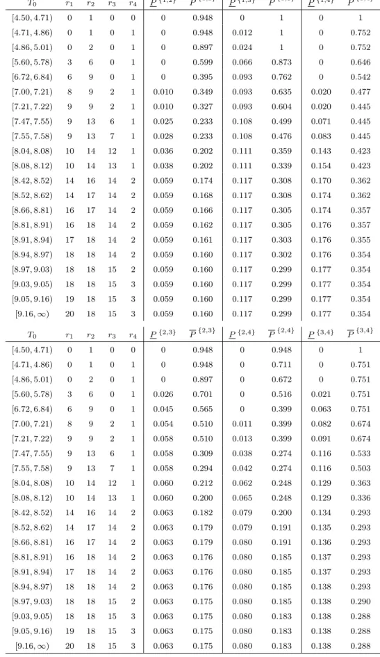
groups, with the assumption that both groups are completely independent. These lower and upper probabilities are given in Table 2.3 and Figure 2.2.

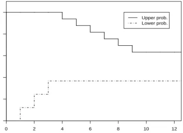
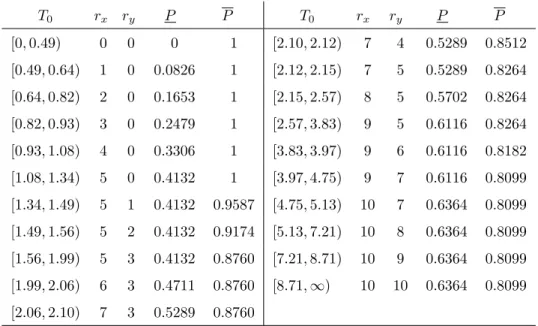
T0 rx ry P P T0 rx ry P P [0,0.49) 0 0 0 1 [2.10,2.12) 7 4 0.5289 0.8512 [0.49,0.64) 1 0 0.0826 1 [2.12,2.15) 7 5 0.5289 0.8264 [0.64,0.82) 2 0 0.1653 1 [2.15,2.57) 8 5 0.5702 0.8264 [0.82,0.93) 3 0 0.2479 1 [2.57,3.83) 9 5 0.6116 0.8264 [0.93,1.08) 4 0 0.3306 1 [3.83,3.97) 9 6 0.6116 0.8182 [1.08,1.34) 5 0 0.4132 1 [3.97,4.75) 9 7 0.6116 0.8099 [1.34,1.49) 5 1 0.4132 0.9587 [4.75,5.13) 10 7 0.6364 0.8099 [1.49,1.56) 5 2 0.4132 0.9174 [5.13,7.21) 10 8 0.6364 0.8099 [1.56,1.99) 5 3 0.4132 0.8760 [7.21,8.71) 10 9 0.6364 0.8099 [1.99,2.06) 6 3 0.4711 0.8760 [8.71,_∞) 10 10 0.6364 0.8099 [2.06,2.10) 7 3 0.5289 0.8760

Table 2.3: NPI lower and upper probabilities for the eventX₁₁< Y₁₁

Table 2.3 and Figure 2.2 show that, for increasing T0, the lower probability is increasing when rx increases and remains constant when ry increases. The upper

probability remains constant whenrx increases and is decreasing whenry increases,

except for ry ≥ 7 when it remains constant due to xnx < yry+1 for such ry, which illustrates Theorem 2.3. The imprecision is decreasing when more lifetimes are observed. However, if T0 ≥ 4.75, increasing ry while keeping rx constant does not

lead to less imprecision due to the fact that at that time we have observed all lifetimes of group X (xnx < yry+1) and consequently increasing ry will not give us more information about the ordering of the lifetimes of groupsX and Y.

One could interpret P(X11< Y11)> 1₂ as a strong indication that indeed X11 <

Y11. From Table 2.3 we see that if we had stopped the experiment at T0 = 2.06 or later, then indeed P(X11 < Y11) > 1₂. Had the experiment been stopped earlier,

(38)

2.5. Examples 29 0 2 4 6 8 0.0 0.2 0.4 0.6 0.8 1.0 T0 Probability Upper prob. Lower prob.

Figure 2.2: NPI lower and upper probabilities for the eventX11< Y11

then the NPI lower and upper probabilities would not suggest a strong preference between the groups.

To compare this with the classical precedence tests, we test H0 : FX = FY

against the alternative hypothesis that FX(x) ≥ FY(x) for x ≥ 0, with strict

in-equality for some x. Table 2.4 gives the values of the test statistics and the cor-responding p-values (between brackets) for ry = 1, . . . ,6, where the restriction to

these values of ry is chosen as these illustrate all relevant issues in the discussion.

ry 1 2 3 4 5 6 Q(ry) 5 (0.016) 5 (0.070) 5 (0.175) 7 (0.089) 7 (0.185) 9 (0.070) U(ry) 5 (0.016) 5 (0.033) 5 (0.049) 5 (0.065) 5 (0.081) 5 (0.097) Wmin,ry 60 (0.016) 65 (0.022) 70 (0.033) 73 (0.031) 76 (0.035) 77 (0.029) WE,ry 82.5 (0.016) 85 (0.036) 87.5 (0.067) 82 (0.035) 83.5 (0.048) 79 (0.025) Wmax,ry 105 (0.016) 105 (0.036) 105 (0.086) 91 (0.041) 91 (0.065) 81 (0.024)

Table 2.4: Several nonparametric precedence tests

Table 2.4 shows that the classical precedence test will not reject the null hy-pothesis of equal distributions at 5% significance level except when the experiment is terminated after the first lifetime of group Y. The maximal precedence test will reject the null hypothesis if the experiment is terminated after at most 3 lifetimes

(39)

2.6. Concluding remarks 30

of groupY. Intuitively, this is logical as we have first observed 5 lifetimes of group

X before the first observation of group Y and no observed lifetimes of group X

between the first and third observation of group Y. In this example, Wilcoxon’s minimal rank-sum precedence test always rejects the null hypothesis at 5% signifi-cance level. However, Wilcoxon’s maximal and expected rank-sum precedence tests reject the null hypothesis only for some values ofry. We saw before that according

to our NPI approach there is an indication that X11 < Y11 when the experiment is terminated after T0 = 2.06. The results of the classical, Wilcoxon’s maximal and expected rank-sum precedence tests at this T0 are not in agreement with this but the maximal and Wilcoxon’s minimal rank-sum precedence tests are. As the NPI approach is fundamentally different to these hypothesis tests, studying the results

of both might provide useful insights for practical problems. ₄

2.6

Concluding remarks

The lower and upper probabilities for predictive precedence testing for two groups, presented in this chapter, fit in the NPI framework and as such they have strong con-sistency properties in theory of interval probability [1]. This approach provides an attractive alternative to the more established methods for nonparametric precedence testing [5], as instead of testing a null hypothesis the inference directly considers a comparison of the next observations from the groups considered.

When considering the NPI lower and upper probabilities for the event Xnx+1 <

Yny+1 as a function of the stopping time T0, we showed that these probabilities can only change at observed lifetimes for groupsX orY. In particular, we showed that, except for one special case, the lower probability is strictly increasing in rx while

keeping ry constant, and the upper probability is strictly decreasing in ry while

keeping rx constant. As a consequence of this, the imprecision is decreasing as a

function of the number of observed lifetimes and hence as a function of time. An important issue in statistics is guidance on required design of experiments, in this situation the numbers of units to be used for both groups and choice of the stopping time for the experiment. Due to the rather minimal assumptions

(40)

2.6. Concluding remarks 31

underlying our NPI approach, with the inferences largely based on observed data, it does not offer a satisfactory solution to this important question. However, once an experiment is underway, one can monitor the lower and upper probabilities as presented in this chapter, and one can stop the experiment if one judges these to indicate a strong enough preference between the two groups. Of course, before any data become available, one can study some design issues, e.g. the minimum required number of observations to possibly get a lower probability greater than a half, but as these would be based on most or least favourable configurations of the not yet observed data, indications from such studies might be of little practical value.

(41)

Chapter 3

Multiple comparisons with early

termination

3.1

Introduction

In Chapter 2 we introduced NPI for comparison of two groups with early termination of experiments. In this chapter, we consider the situation where units from several groups (k ≥2) are simultaneously placed on a life-testing experiment, and decisions may be needed before all units have failed due to cost or time considerations.

Balakrishnan and Ng [5] described several nonparametric precedence tests based on the hypothesis of equal lifetime distributions. In Section 3.2 we briefly describe some of these classical methods. In Sections 3.3, 3.4 and 3.5 we present NPI for precedence testing for k _≥ 2 groups in order to select the best group, the subset of best groups and the subset including the best group, respectively. Examples are provided throughout to illustrate our method and to compare it with the classical methods. Section 3.6 contains some concluding remarks.

3.2

Classical methods

When the null hypothesis of the equality (homogeneity) of two (or more) popu-lations (e.g. processes, treatments) is rejected, one may want to identify which of these populations is the best. Balakrishnan and Ng [5] introduced several

(42)

3.2. Classical methods 33

metric tests for this selection problem when an early decision is required (called precedence testing). Below we briefly describe these precedence selection methods using notation and definitions from Balakrishnan and Ng [5].

Suppose that we have independent random samples from k _≥ 2 different

pop-ulations. Let Xj,ij (ij = 1, . . . , nj) be the lifetime of the ijth component of a ran-dom sample from population πj with distribution function Fj (j = 1, . . . , k). We

have N = Pk

j=1nj units placed simultaneously on a lifetime testing experiment. The question of interest is to test whether these populations are homogeneous, i.e.

H0 : F1 = F2 = . . . = Fk against the alternative that population πi is the best

(longer life), that isHAi :Fi < Fj for allj 6=i and j = 1, . . . , k. That is, it can be

concluded thatXi, a random quantity representing the lifetime of a unit of

popula-tion i, is stochastically larger than Xj (i.e. Xi st Xj) if and only if Fi(x)≤ Fj(x)

for all x≥0 with strict inequality for at least onex, consequently Fi < Fj.

In precedence testing the aim is to reach a decision before all units have failed. So the experiment is terminated as soon as the ¯rith failure from groupiis observed,

where ¯ri = bniqc for i = 1, . . . , k and 0 < q < 1, where bac is the largest integer

not greater than a. Consequently, the stopping time T0 can be defined as T0 = min

1≤i≤kXi,(¯ri), where Xi,(¯ri) is the ¯rith order statistic of sample i.

Suppose now that the experiment is terminated at sample i, i.e. T0 = Xi,(¯ri), then the ordinary precedence statistic [6] is defined as

Q∗(i)= min 1≤j≤k j6=i Q(_ji)/nj (3.1)

where Q(_ji) is the number of failures observed before Xi,(¯r) from the sample j (j = 1, . . . , k, j 6= i). Small values of Q∗(i) _{will lead to rejection of the null hypothesis}

H0. In this case one can choose HAj (πj is the best) if and only if (Qj(i)/nj) =Q∗(i)

forj 6=i and T0 =Xi,(¯ri). If for two or more samples the statistic (Q (i)

j /nj) is equal

toQ∗(i) _{then one of the corresponding populations is randomly selected as the best.} Now letD_j,s(i)be the number of failures of samplejthat occur between the (s−1)th and sth failure of group i, s = 2, . . . ,r¯i and let D(j,i1) be the number of failures of samplej that occur