Experiments to Parameters and Base Classifiers in the Fitness Function for GA-Ensemble

(1)

Experiments to Parameters and Base Classifiers in the Fitness

Function for GA-Ensemble

Dong-Yop Oh

*

Department of Information Systems, The University of Texas Rio Grande Valley, Edinburg, TX 78539-2999, USA

Abstract: GA-Ensemble is found to be more resistant to outliers and results in simpler predictive models than other ensemble models. The fitness function consists of three parameters (a, b, and p) that limit the number of base classifiers (by b) and control the effects of outliers (by a) to maximize an appropriately chosen p-th percentile of margins. We present the effect of the parameters of a new fitness function as well as the increased complexity of base classifiers to improve predictive accuracy. We use some artificial and real data sets to demonstrate the effect of GA-Ensemble performance at 16 different treatment levels with three different base classifier options and compare to AdaBoost. Keywords: AdaBoost, Classification, Ensemble, Genetic algorithm, Predictive model.

1. INTRODUCTION

The recent methods with respect to classification problems are able to handle large data sets easily without many assumptions. A single decision tree is useful in identifying complex interactions among predictors compared to classical methods. However, it is unstable and its performance is not very good compared to more recent methods. Ensemble methods like boosting [1] and random forests [2] can improve predictive model performance but have complex interpretations and computation problems. The performance of these techniques strongly depends on the data characteristics. As a result, there is no best method for all problems.

Boosting is a widely used and powerful prediction technique that sequentially constructs an ensemble of base classifiers for a binary classification problem. In some experiments (e.g., [3-5]), empirical results suggest that boosting often does not overfit even with thousands of rounds. Nevertheless, the actual performance of boosting is dependent on the data set and the base classifier. So there is still an overfitting problem because boosting is sensitive to unusual examples in the data in trying to attain a perfect fit to the training data [6-9].

One of the main issues in boosting is to study the properties of the margin distribution in order to get better generalization performance. Schapire et al. [10] discussed methods for improving performance related

*

Address correspondence to this author at the Department of Information Systems, The University of Texas Rio Grande Valley, Edinburg, TX 78539-2999, USA; Tel: (956) 665-3314; Fax: (956) 665-3367;

E-mail: [email protected]

to the distribution of margins of the training data. Their experiments show that there is a good correlation between a reduction of the portion of training examples having a small margin and generalization performance. They also show that increasing the margins is very effective theoretically and experimentally. Breiman [11] presented that arc-gv produces a higher margins distribution than AdaBoost [12], but the performance is worse. Reyzin and Schapire [13] argued that worse performance of Breiman’s experiments can be explained by the increased complexity of the base classifiers.

Oh and Gray [14] proposed GA-Ensemble to solve the over fitting problem by maximizing the p-th percentile of the margin or ignoring the p-th percentile of the smallest margin. GA-Ensemble simplifies the interpretation of the final model by penalizing the model complexity term as measured by the number of base classifiers in the fitness function. However, further study is needed about choosing p for maximizing p-th percentile and combination of the parameters (a and b)

in the fitness function to determine good settings. Oh and Gray [15] used a plot of margins as opposed to p

maximized, but the tuning parameters (a and b) in the fitness function do not represent optimal combinations. This paper focuses on the effect of the increased complexity of base classifiers and determining how to find the best values of the tuning parameters for different data sets to control the number of base classifiers and maintain outlier resistance.

After reviewing GA-Ensemble algorithm in Section 2, we present designed experiments with 16 treatment levels to find the best parameters and introduce three different base classifiers in Section 3. We discuss the effect of the parameters of a new fitness function as

(2)

well as the increased complexity of base classifiers based on simulation and real data sets in Section 4. Section 5 contains a summary and discussion.

2. ALGORITHM AND NEW FITNESS FUNCTION

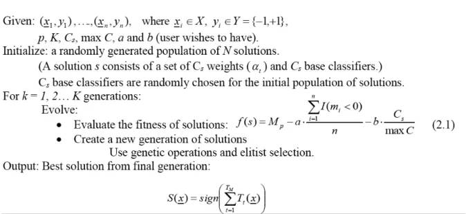
The GA-Ensemble algorithm is a method for optimizing base classifiers and their weights, which are randomly generated, using a genetic algorithm. Figure 1 presents a GA-Ensemble algorithm. In this genetic algorithm, a solution is a set of base classifiers and their weights. On each generation, solutions are evaluated by the fitness function in (2.1), and a new generation of solutions evolves through genetic operations (mutation, crossover, grow, and prune) and elitist selection. The fitness function can measure the goodness of each solution and after K generations the final solution, which is a combination of base classifiers with their weights optimized, is chosen in the final generation with the largest fitness value. Therefore GA-Ensemble simultaneously optimizes the weights, split variables, split values, and predictions by a genetic algorithm. During processing, the number of base classifiers is limited by utilizing the tuning parameter b, Cs, maxC, and crossover operation.

The fitness function (2.1) of a genetic algorithm is consist of the p-th percentile of the margin distribution with two penalty terms for the misclassification rate and the model complexity measured by the number of base classifiers. From the first term, Mp, we can identify or

ignore outliers using the margins of training data. The margin has a range of [-1, +1] which is positive if and only if the final model correctly classifies the training set. The magnitude of the margin is interpreted as a measure of confidence in the prediction. Therefore outliers usually have a large negative margin. The fitness function ignores the p% of the smallest margins but considers maximizing the p-th percentile of margin, so that we have a more outlier resistant solution.

Through the penalty term for the number of negative margins, not only the performance of the algorithm would be improved, but also we can maintain outlier resistance when p% is less than the proportion of outliers in the training data. To construct a simpler model combined with distinct base classifiers, the fitness function is penalized with respect to complexity as measured by the number of base classifiers in order to reduce the computation and interpretation problems.

The tuning parameters a and b are the tuning parameters for the penalties on the number of negative margins and the number of base classifiers in the new fitness function of the genetic algorithm. They can be chosen to avoid one or two of the three terms in the fitness function dominating the others so that it makes sense to normalize the terms to make interpretations and the choice of a and b easier. The range of the first term is from -1 to +1 and the second term is the training error laid between 0 and 1. The third term is divided by maxC, the size of the largest solution the

Figure 1: GA-Ensemble algorithm. (2.1) is the fitness function where M_p is the p-th percentile of the margin distribution, I(•) is an indicator function, m_i is the i-th margin, n is the number of observations, Cs is the number of base classifiers in the solution s,

(3)

user wishes to have (Note: It is still possible for a solution to be larger than maxC; it is simply a reference point for normalizing Cs). Therefore third terms tend to lie between 0 and 1 although it is possible for the third term to exceed 1.

With regard to interpretation, the choice of a (or b) represents a trade-off. In the case of a, an increase of g

units in Mp is regarded as equivalent to an increase of g/a units in the training error, with regard to the fitness function. Likewise, in the case of b, an increase of g

units in Mp is regarded as equivalent to an increase of g/b units in the normalized size of the solution.

3. DESIGNED EXPERIMENTS AND BASE CLASSIFIERS

To find the best combination of tuning parameters based on the different data sets, we need to set up the designed experiment on three factors: p, a, and b. Because the best combination of a, b, and p depends on the data structure, and it is impossible to test all values of p, a, and b, we designed a simulation experiment to study the effects of those parameters. First we set the maximizing percentile of the margins,

p, to 0.0 (0%), 0.05, 0.10, and 0.15. The value of p = 0.0 corresponds to maximizing the minimum margin. We set the values of a to 1.0 or 5.0 and b to 0.1 or 0.5 so that there are four different combinations (a, b): (1.0, 0.1), (1.0, 0.5), (5.0, 0.1) and (5.0, 0.5) with 4 different values of p, which are 0.00, 0.05, 0.10, and 0.15. Therefore this designed experiment on three factors leads to 16 treatments for GA-Ensemble. Table 1

displays the 16 treatments of the tuning parameters, a, and b with the value of p indicating which percentile to maximize. We have a consistent convergence value of fitness with 2000generations for all data sets. For each simulation data set, we have 10 replicated runs per treatment. In this paper we show the designed

simulation experiments on the effects of parameters, to see that there are some general recommendations that might be made about their choice.

To extend the base classifiers beyond stump trees (one split with two terminal nodes), we considered decision trees with three split points and oblique stump trees for GA-Ensemble. Decision trees with three split points are randomly produced and evolve into one of three different types of trees, which have either two terminal nodes with one split point (stump), or three terminal nodes with two split points, or four terminal nodes with three split points. A stump tree can split data sets vertically or horizontally, but a stump tree with linear combination splits (also known as "oblique splits") can split obliquely as well as vertically or horizontally in the predictor space. So a two-terminal node, oblique stump tree is similar to a stump tree, but it is a more complicated and general model than a stump. The base classifiers with their weights are randomly chosen for the initial population of solutions and optimized by genetic operations.

4. EXAMPLES

In this section, two artificial data sets and three real data sets are used to demonstrate the effect of increased complexity of base classifiers, and how to find the best values of the tuning parameters to control the number of base classifiers and maintain outlier resistance. We also compare GA-Ensemble with 16 treatments to AdaBoost with 8 different values of the number of iterations (T). As default values, we set Cs = 5, the initial number of base classifiers in the 20 initial solutions (N = 20), and maxC = 20, the maximum number of base classifiers in a solution. The number of simulations in the genetic algorithm is K = 2,000.

Table 1: Treatment Levels of Designed Experiments

Treatment 1 2 3 4 5 6 7 8 p 0.00 0.00 0.00 0.00 0.05 0.05 0.05 0.05 a 1.0 1.0 5.0 5.0 1.0 1.0 5.0 5.0 b 0.1 0.5 0.1 0.5 0.1 0.5 0.1 0.5 Treatment 9 10 11 12 13 14 15 16 p 0.10 0.10 0.10 0.10 0.15 0.15 0.15 0.15 a 1.0 1.0 5.0 5.0 1.0 1.0 5.0 5.0 b 0.1 0.5 0.1 0.5 0.1 0.5 0.1 0.5

(4)

4.1. The First Simulation

For the first simulation, a d = 2-dimension problem with sample size n=100 is considered. Two predictor values are randomly generated from a uniform [0, 1] distribution. We have a response variable, Y

!

{-1, +1}

given by Y= ₊₁ _otherwise. !1 for x1"0.05 and x2#0.05 $ % & '& ( ) & *& (3.1)

To look at the effect of noise, we add 10% random noise to the data set and display the effect on GA-Ensemble with various p-th percentiles to be maximized and the tuning constants, a and b, in the fitness function of the genetic algorithm. Stump trees with two terminal nodes were used as base classifiers for GA-Ensemble and AdaBoost. Intuitively we expect that few stumps are needed to correctly classify for a simple simulation data, so we assign a larger penalty b

for the number of base classifiers in the fitness function to produce a simple solution.

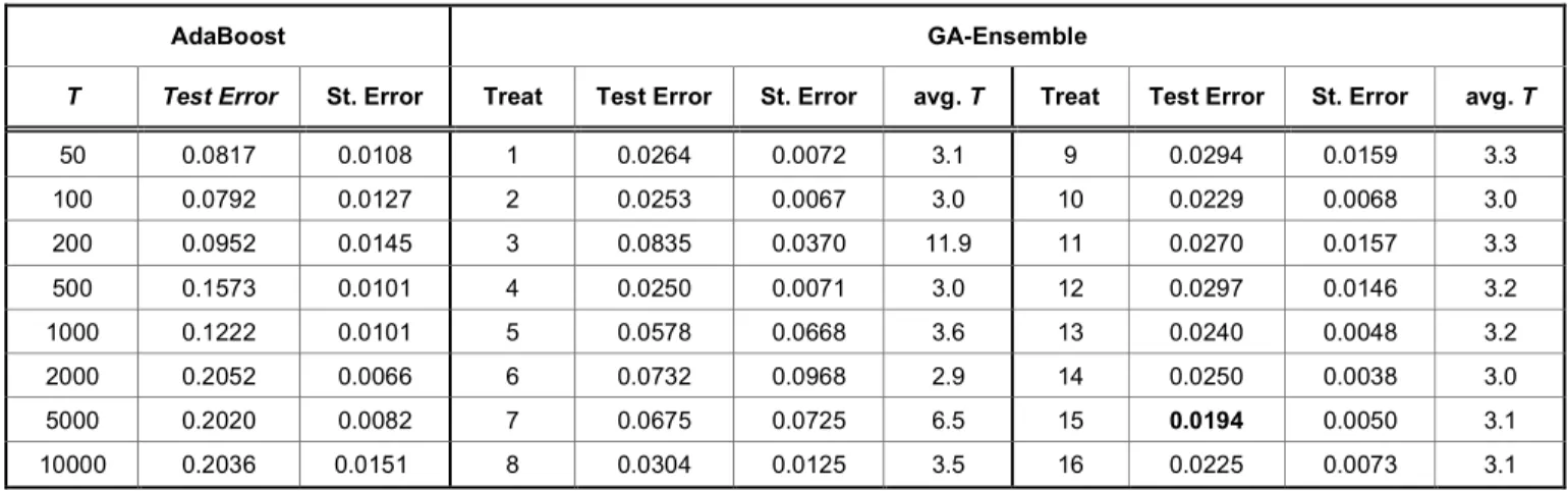
Now we want to compare GA-Ensemble for the 16 treatments shown in Table 2 to AdaBoost with different numbers of iterations (T= 50, 100, 200, 500, 1,000, 2,000, 5,000, and10,000) based on the simple data set

I with 10% noise, and to evaluate the performance using a test set (n=10,000).

The test error of AdaBoost when T = 100 goes down to 0.0792 and then up as the number of iterations increases. The smallest test error among those is 0.0792, which is not better than any test errors from GA-Ensemble with 16 treatment levels. The bold number, 0.0194, which is from GA-Ensemble

maximizing the 15th percentile of margins with a=5.0, b

= 0.1, indicates the best performance with using 3.1 stumps. The outliers are ignored by the GA-Ensemble solution and are misclassified, as they should be in an outlier-resistant solution. Thus GA-Ensemble provides a simpler solution that looks more like the original population of rectangular data and is more resistant to outliers than AdaBoost.

In addition, we can determine that the final solution with a large number of classifiers is not worth classifying the simple data. In treatment 3 with a=5,

b=0.1, and p=0.00, GA-Ensemble produces 11.9 averaged stumps, which is the largest number of classifiers, but the performance is the poorest among the 16 treatments based on a data set with 10% noise. Most of the test errors are less than 0.03 or around 0.03 except treatments 3 and 7 so that the effect of tuning parameters is not respected for the simple data. The best and the worst are from treatment 15 and 3, respectively; these have the same combination (5.0, 0.1) of a and b but p is different (0.15, 0.0, respectively). So to classify the data sets with noise, it is a good idea to utilize a value of p that is greater than the noise level. Furthermore, the size of p may affect the number of classifiers for the noise data when the trim size is less than the noise level as in treatment 3 and 7.

4.2. The Second Simulation

The second artificial data set is generated from a concentric circles structure which has been used already in many papers (e.g., [14]). We employed a two-dimensional concentric circle structure and predictors are arbitrarily generated from a uniform distribution on the interval [-1, 1] with n=300

Table 2: Test Errors for AdaBoost with Different Iterations (T=50, 100, 200, 500, 1,000, 2,000, 5,000, and 10,000)and GA-Ensemble with 16 Treatments Based on First Simulation Data with 10% Noise Level. Bold Indicates the Best Result between AdaBoost and GA-Ensemble

AdaBoost GA-Ensemble

T Test Error St. Error Treat Test Error St. Error avg. T Treat Test Error St. Error avg. T

50 0.0817 0.0108 1 0.0264 0.0072 3.1 9 0.0294 0.0159 3.3 100 0.0792 0.0127 2 0.0253 0.0067 3.0 10 0.0229 0.0068 3.0 200 0.0952 0.0145 3 0.0835 0.0370 11.9 11 0.0270 0.0157 3.3 500 0.1573 0.0101 4 0.0250 0.0071 3.0 12 0.0297 0.0146 3.2 1000 0.1222 0.0101 5 0.0578 0.0668 3.6 13 0.0240 0.0048 3.2 2000 0.2052 0.0066 6 0.0732 0.0968 2.9 14 0.0250 0.0038 3.0 5000 0.2020 0.0082 7 0.0675 0.0725 6.5 15 0.0194 0.0050 3.1 10000 0.2036 0.0151 8 0.0304 0.0125 3.5 16 0.0225 0.0073 3.1

(5)

observations. A response variable, Y !{-1, +1}, is given by Y =sign k

(

!!! sin(x₁2+x₂2)

)

, and Y is equal to

-1 if y_i is less than the median of x₁2+x₂2 and +1

otherwise. Therefore the data set has the same number of observations in each class, 150 for constructing the models and 5,000 observations are generated for the test. Decision trees with one and three split points and linear combination splits are employed as base classifiers to build the final model.

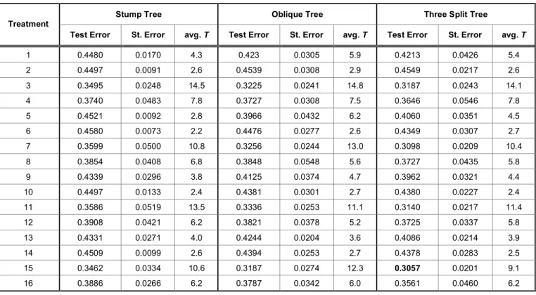
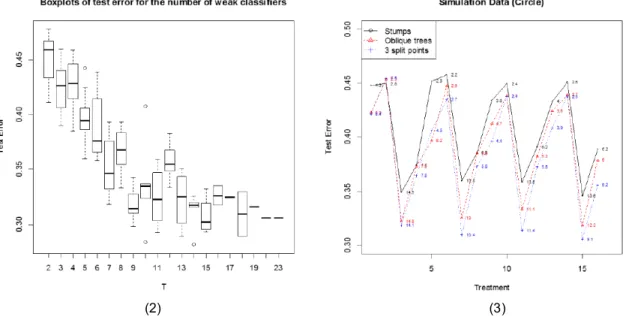
The circle data is more complex for correctly classifying all training data than the first simulation data set. In Table 3 and Figure 3, we see that treatments 2, 6, 10 and 14 which have 1.0 and 0.5 for a and b have a worse performance with over 0.435 misclassification rate. The final solutions from those treatments have two or three classifiers, which are not enough to classify this complicated data set well. We observe that the best treatments are 3, 7, 11, and 15, which averaged 8, 9, or 10 base classifiers in the final solution. They performed significantly better than other solutions with 2 or 3 classifiers and slightly better than all other treatments with solutions having 4 and 5 classifiers. In Figure 2 we can compare the number of classifiers in the final solutions in terms of test errors. We can also infer which combinations of parameters have the best performance. For example, if we need 15

base classifiers for a final model, we can verify that treatment 3 is the best way to produce 15 base classifiers to classify examples. Therefore in order to classify a complex data set, we need the final solution to include more base classifiers. To do that, we put a small value of the tuning constant b for the number of base classifiers in the fitness function.

Table 3 provides a summary of GA-Ensemble for decision trees with one and three split points, and oblique stump trees based on the circle data set. Obviously, GA-Ensemble for 3 split points tends to produce a better result than for stumps and oblique stump trees, and GA-Ensemble for oblique trees achieves better performance than for stumps. Table 4

presents the win-tie-loss for all pairwise combinations of three base classifiers. When we compare decision trees with 1 split point and oblique stump trees to decision trees with 3 split points, we see that decision trees with 3 split points are superior to the others (15-0-1, 14-0-2), but in treatments 2 and 5, decision trees with 3 split points are inferior to oblique stump trees. In comparing decision trees with one split point to oblique stump trees, we can see oblique stump trees beat decision trees with one split point in all treatments (15-0-1) except treatment 2. From this result, we conclude that the best base classifier with the circle data is a decision tree with 3 split points. Decision trees with 1

Table 3: Test Errors (Standard Errors) of each Treatment for Decision Tree with one and Three Split Points, and Oblique Stump Trees Based on the Circle Data Set

Stump Tree Oblique Tree Three Split Tree Treatment

Test Error St. Error avg. T Test Error St. Error avg. T Test Error St. Error avg. T

1 0.4480 0.0170 4.3 0.423 0.0305 5.9 0.4213 0.0426 5.4 2 0.4497 0.0091 2.6 0.4539 0.0308 2.9 0.4549 0.0217 2.6 3 0.3495 0.0248 14.5 0.3225 0.0241 14.8 0.3187 0.0243 14.1 4 0.3740 0.0483 7.8 0.3727 0.0308 7.5 0.3646 0.0546 7.8 5 0.4521 0.0092 2.8 0.3966 0.0432 6.2 0.4060 0.0351 4.5 6 0.4580 0.0073 2.2 0.4476 0.0277 2.6 0.4349 0.0307 2.7 7 0.3599 0.0500 10.8 0.3256 0.0244 13.0 0.3098 0.0209 10.4 8 0.3854 0.0408 6.8 0.3848 0.0548 5.6 0.3727 0.0435 5.8 9 0.4339 0.0296 3.8 0.4125 0.0374 4.7 0.3962 0.0321 4.4 10 0.4497 0.0133 2.4 0.4381 0.0301 2.7 0.4380 0.0227 2.4 11 0.3586 0.0519 13.5 0.3336 0.0253 11.1 0.3140 0.0217 11.4 12 0.3908 0.0421 6.2 0.3821 0.0378 5.2 0.3725 0.0337 5.8 13 0.4331 0.0271 4.0 0.4244 0.0204 3.6 0.4086 0.0214 3.9 14 0.4509 0.0099 2.6 0.4394 0.0253 2.7 0.4378 0.0283 2.5 15 0.3462 0.0334 10.6 0.3187 0.0274 12.3 0.3057 0.0201 9.1 16 0.3886 0.0266 6.2 0.3787 0.0342 6.0 0.3561 0.0460 6.2

(6)

split point are not good choices for base classifiers. We can also verify these results in Figure 3, which shows the plot of test error for 16 treatments along with three different base classifiers. The solid line (black) is from the decision tree with one split point, the dashed line (red) is from the oblique tree, and the dotted line (blue) is from the decision tree with 3 split points based on the circle data. Labeling points are the average numbers of base classifiers (T).

Treatments 2, 6, 10, and 14, which have a large value of b (= 0.5), have worse outcomes with 2 or 3 base classifiers. The best performances are achieved with a large T in treatments 3, 7, 11, and 15 for all three different base classifiers. This clearly indicates that more base classifiers and more complicated base classifiers are needed for a difficult to classify data set such as circle data. The first four treatments are based on maximizing the minimum margin and the next four on maximizing the 5th percentile of the margins, followed by the 10th and 15th percentiles of margins for the remaining treatments. As for stumps, four different levels of p seem not to be significantly different from the results for decision trees with 3 split points and

oblique trees because we did not find any differences in the different levels of p in Table 3. However, we observed that the tuning parameter b has a strong influence on the results. The value of b = 0.1 produces better results than b = 0.5 and the combinations of (a,

b) = (5.0, 0.1) would be selected for the circle data set among 16 treatments regardless of the four different values of p(0.00, 0.05, 0.10, and 0.15).

4.3. Application to Real World Data

For the real world applications we used three data sets from the UCI Machine Learning Repository: kyphosis data (81, 3), glaucoma data (196, 62), and Wisconsin Diagnostic Breast Cancer data (569, 30). The number of observations and predictors are displayed, respectively, in parentheses. We used 10-fold cross-validation for reporting testing set accuracy. Sixteen treatments of the tuning parameters, a and b

with the value of p to maximize, were tested for GA-Ensemble, which evolved solutions for 2,000 generations on the training set to get the best solution over the 10 runs for each treatment. The more generations in the genetic algorithm, the better fitness

Table 4: Each Cell Contains the Number of Wins, Ties, and Losses between the Base Classifier in that Row and the Base Classifier in that Column for the Circle Data

DT with 1 Split Point Oblique Stump Tree

Oblique Stump Tree 15-0-1

DT with 3 split points 15-0-1 14-0-2

(2) (3)

Figure 2: Boxplots of test error for the number of oblique stump trees in a final solution (left).

Figure3:The plot of test errors for 16 treatments with three different base classifiers based on the second simulation data. Labeling points are the average number of base classifiers out of 10 runs (right).

(7)

value we have. The number of generations, 2,000, is not sufficientto get a convergence of the fitness value for large data sets, especially for the Wisconsin Diagnostic Breast Cancer data. Because it is too expensive to run-time using a current computer program, we used 2,000 generations to construct the best solution for all real data sets. In the initial random solution, we set the number of random base classifiers and their weights to five. The results of running the three different base classifiers (decision trees with two terminal nodes and three split points, and an oblique stump tree) are shown for GA-Ensemble in Tables 6, 7, and 8. Bold numbers indicate the best generalization

performance among all treatments from the three different base classifiers. The results from AdaBoost based on decision tree stumps as a base classifier are shown in Table 5. To be fair, the comparison between the test errors generated by AdaBoost and GA-Ensemble is for one split decision trees.

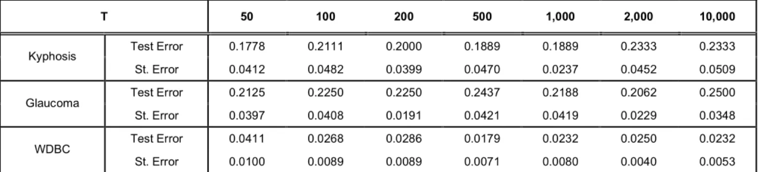
For the kyphosis data, the test errors from AdaBoost are 0.1778 to 0.2333 according to the number of iterations in Table 5. We can see that the performance is best at T = 50 and worst at T = 2,000, and 10,000. AdaBoost with T = 50 is also the best performance and with T=10,000 is worst for the

Table 5: 10-Fold Cross Validation (Standard Errors) from AdaBoost (T=50, 100, 200, 500, 1,000, 2,000, and 10,000)for Decision Trees with one Split Point (Stump) Based on the Kyphosis, Glaucoma, and WDBC Data Sets

T 50 100 200 500 1,000 2,000 10,000 Test Error 0.1778 0.2111 0.2000 0.1889 0.1889 0.2333 0.2333 Kyphosis St. Error 0.0412 0.0482 0.0399 0.0470 0.0237 0.0452 0.0509 Test Error 0.2125 0.2250 0.2250 0.2437 0.2188 0.2062 0.2500 Glaucoma St. Error 0.0397 0.0408 0.0191 0.0421 0.0419 0.0229 0.0348 Test Error 0.0411 0.0268 0.0286 0.0179 0.0232 0.0250 0.0232 WDBC St. Error 0.0100 0.0089 0.0089 0.0071 0.0080 0.0040 0.0053

Table 6: Test Errors (Standard Errors) with Average T of each Treatment for Decision Trees with one and Three Split Points and Oblique Stump Trees Based on the Kyphosis Data. Test Errors are Estimated by 10-Fold Cross-Validation

Stump Oblique Decision Tree

Treatment

1 0.3083 0.3012 3.1 0.2847 0.1876 9.8 0.2736 0.2883 3.7 2 0.2333 0.1574 2.2 0.2083 0.0962 2.9 0.2236 0.1003 2.4 3 0.3222 0.1364 4.6 0.2111 0.0627 8.7 0.2111 0.1335 5.2 4 0.2708 0.1262 3.1 0.2347 0.1608 5.7 0.2972 0.0675 4.4 5 0.2458 0.1280 2.9 0.2111 0.1043 5.8 0.1750 0.1344 3.2 6 0.2583 0.1054 2.3 0.2361 0.1724 2.7 0.2250 0.1748 2.5 7 0.2361 0.1258 4.6 0.1972 0.1459 6.7 0.2208 0.1905 9.2 8 0.2208 0.0922 3.6 0.1972 0.1459 5.8 0.2611 0.1261 4.3 9 0.3333 0.2430 3.3 0.2111 0.1876 3.6 0.2361 0.0735 4.3 10 0.2208 0.1094 2.4 0.2125 0.1773 2.6 0.2000 0.1344 2.6 11 0.3083 0.1574 5.6 0.2097 0.1444 6.4 0.2611 0.1392 5.4 12 0.2222 0.0982 4.1 0.2083 0.1632 3.9 0.1736 0.1350 4.6 13 0.1708 0.1280 2.8 0.2125 0.1449 2.4 0.2236 0.0811 2.1 14 0.2194 0.1657 2.6 0.2000 0.1687 2.2 0.2236 0.1431 1.8 15 0.2250 0.3107 2.6 0.2097 0.1318 3.6 0.2722 0.1653 4.0 16 0.1847 0.1202 2.8 0.1861 0.1223 2.1 0.2708 0.1262 1.9

(8)

glaucoma data. AdaBoost has the worst performance at T=10,000 for both data sets. In other words, using a large number of base classifiers does not produce better results. Based on the WDBC data, AdaBoost has the best performance at T = 500 and the worst at T = 50.

Tables 6, 7, and 8 provide a summary of GA-Ensemble on the 16 treatments with three different base classifiers. Here we consider the one split point decision tree to compare with AdaBoost performance. The 16 treatments resulted in better interpretability, with fewer than 12 base classifiers on average in a final solution than the final model from AdaBoost for three data sets. For the kyphosis, 8 of 16 treatments have less than 3 stumps. Treatment 11 has the largest average number of base classifiers (T= 5.6) but not a very good result in terms of test set error. GA-Ensemble on treatment 13 with 2.8 average base classifiers did the best compared to AdaBoost. Treatments 8, 10, 12, 13, 14, 15, and 16 have better performance than AdaBoost with

T= 2000 and 10,000. The remaining treatments are inferior to AdaBoost. When we compare for the glaucoma data, GA-Ensemble on treatments 8, 12, and 16 has better performance than the best of AdaBoost

with T=2,000. Finally, for the WDBC data, we compare GA-Ensemble to AdaBoost based on decision trees with one split point. Results show that AdaBoost had better performance than GA-Ensemble on all 16 treatments for WDBC data. Because this data set is relatively large with n=569 and p=30, 2000 generations may not be enough to construct a good solution. Nevertheless, GA-Ensemble has a strong advantage of interpretation of its final models over AdaBoost. In addition, the WDBC data has low data complexity and contamination. Oh and Gray [14] showed that AdaBoost performs very well and better than GA-Ensemble in the case of low contaminated data. From these comparisons, we can conclude that GA-Ensemble is superior to AdaBoost for the glaucoma and inferior for the WDBC data. For the kyphosis data, they are somewhat equally matched. However, the final models with a few base classifiers by GA-Ensemble have a significant interpretability advantage over those by AdaBoost.

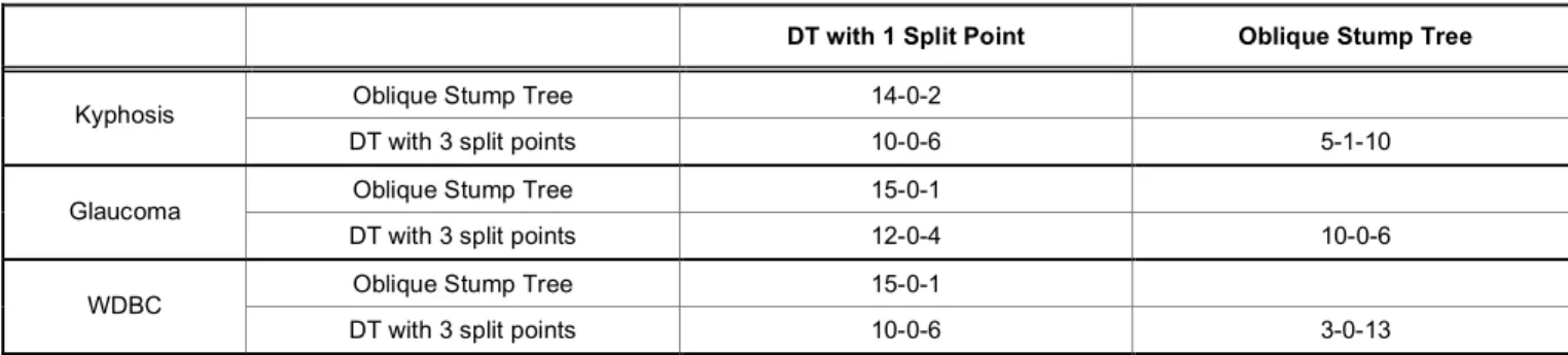
Now we consider more complex base classifiers than stump trees. In Tables 6, 7, and 8, we can see how GA-Ensemble works with different base classifiers and, in Table 9 we can compare the win-tie-loss for all pairwise combinations of three base classifiers. We

Table 7: Test Errors (Standard Errors) with Average T of each Treatment for Decision Trees with one and Three Split Points and Oblique Stump Trees Based on the Glaucoma Data. Test Errors are Estimated by 10-Fold Cross-Validation

1 0.2963 0.2552 3.6 0.2288 0.0862 12.2 0.2550 0.1817 5.2 2 0.2400 0.2221 2.9 0.2387 0.1001 3.0 0.2263 0.1146 3.2 3 0.2213 0.0838 9.8 0.2200 0.0919 18.3 0.1988 0.0625 12.7 4 0.2150 0.1055 4.4 0.1975 0.0989 6.6 0.1888 0.1048 3.7 5 0.2400 0.0738 3.2 0.1837 0.0624 5.1 0.2050 0.0762 3.9 6 0.2575 0.2333 2.3 0.2112 0.1400 2.3 0.2150 0.0973 2.8 7 0.2450 0.0762 11.1 0.2275 0.0837 11.4 0.2038 0.0928 5.9 8 0.1762 0.1152 4.3 0.1525 0.0731 4.5 0.2437 0.0963 3.9 9 0.2462 0.1149 3.9 0.1688 0.0581 6.0 0.2075 0.0764 3.3 10 0.2275 0.0692 2.1 0.1850 0.0784 2.1 0.2162 0.0928 2.1 11 0.2437 0.0934 9.0 0.1950 0.0643 10.2 0.1825 0.1041 8.8 12 0.1963 0.1036 3.9 0.1737 0.0480 4.3 0.1988 0.0944 4.2 13 0.2075 0.1167 2.9 0.2025 0.0885 2.8 0.1938 0.0599 3.3 14 0.2112 0.1203 3.0 0.1825 0.1041 2.8 0.2275 0.0916 3.1 15 0.2125 0.0860 5.2 0.1600 0.0843 6.0 0.1900 0.0615 5.6 16 0.1562 0.1111 3.5 0.1575 0.0708 3.7 0.1888 0.0809 3.3

(9)

expect that the more complex base classifiers with more than two splits and the linear combination splitting rule will work better than stump trees, but computation is more expensive.

For the kyphosis in Table 6 and 9, we see that the best performance with a = 1, b = 0.1, and p = 0.15 is 0.1708 error rate using 2.8 stump trees as an average number of base classifiers. However, the performances of an oblique stump tree are superior to the stump tree (14-0-2) in terms of test set error, except in treatments 13 and 16. Oblique stump tree wins in 10 treatments, loses in 5 and ties in only 1 to the decision tree with 3 split points. Based on the glaucoma data, oblique

stump tree is superior to stump tree and inferior to 3 split points. As shown in Table 7, the test error using 4.5 average oblique stump trees in treatment 8 (with a

= 5, b = 0.5, and p= 0.05) is 0.1525 in Table 7 which is the best effect among all treatments with different base classifiers. Finally, we compare for WDBC. A decision tree with 3 split points has a slight advantage over a stump tree (10-0-6). An oblique stump tree is superior to other base classifiers and the best performance using 4.2 average classifiers is 0.0527 error rates at the treatment 7 with a = 5, b = 0.1, and p = 0.05. The decision trees with one and three split points are inferior to an oblique stump tree (1-0-15 and 3-0-13, respectively).

Table 8: Test Errors (Standard Errors) with Average T of each Treatment for Decision Trees with one and Three Split Points and Oblique Stump Trees Based on the WDBC Data. Test Errors are Estimated by 10-Fold Cross-Validation

Treatment

1 0.0826 0.0343 3.7 0.0704 0.0323 5.4 0.1597 0.2961 3.9 2 0.1317 0.0961 2.9 0.1512 0.1747 2.7 0.0914 0.0529 2.9 3 0.0596 0.0333 8.0 0.0580 0.0310 10.5 0.0685 0.0364 6.8 4 0.0702 0.0104 4.4 0.0632 0.0431 4.4 0.0668 0.0307 2.9 5 0.0598 0.0301 2.9 0.0581 0.0251 2.4 0.0791 0.0323 3.0 6 0.0773 0.0300 2.4 0.0703 0.0167 2.4 0.0632 0.0311 2.7 7 0.0544 0.0345 3.3 0.0527 0.0219 4.2 0.0632 0.0398 3.1 8 0.0720 0.0099 4.3 0.0668 0.0386 3.1 0.0562 0.0284 2.7 9 0.0878 0.0421 1.1 0.0546 0.0309 1.2 0.0914 0.0285 1.2 10 0.0984 0.0322 1.0 0.0862 0.0490 1.2 0.1090 0.0275 1.0 11 0.1055 0.0320 1.2 0.0669 0.0341 1.3 0.0860 0.0448 1.7 12 0.1036 0.0076 4.6 0.0581 0.0407 1.1 0.0843 0.0338 1.0 13 0.0985 0.0346 1.3 0.0704 0.0345 1.1 0.1036 0.0290 1.2 14 0.1002 0.0379 1.0 0.0686 0.0319 1.1 0.0914 0.0437 1.1 15 0.0931 0.0350 1.9 0.0634 0.0347 1.5 0.0895 0.0391 2.0 16 0.0984 0.0083 3.5 0.0685 0.0400 1.4 0.0860 0.0441 1.1

Table 9: Each Cell Contains the Number of Wins, Ties, and Losses between the Base Classifiers in that Row and the Base Classifiers in that Column for the Kyphosis, Glaucoma, and WDBC Data Sets

DT with 1 Split Point Oblique Stump Tree

Kyphosis

Glaucoma

WDBC

(10)

DISCUSSION AND CONCLUSION

We tested the effect of the parameters of a new fitness function and the increased complexity of base classifiers on several data sets including two simulated data sets and three real-world data sets. Our results provide several implications. First, it is a good indication to apply a value of the maximizing p-th percentile of margin,p, that is greater than noise levels and a large (small) value of the tuning constant b to generate less (more) base classifiers for better performance on a simple (complex) data. From comparing GA-Ensemble with 16 treatments to AdaBoost with different numbers of iterations based on stumps as a base classifier, GA-Ensemble provides solutions that are simpler than those found by AdaBoost with better or equal performance. In addition, through comparisons with more complex base classifiers than stump trees, a complex classifier as a base classifier works better than a simple one, but the computational cost will be higher.

Based on the results of the second simulation data, we expected that more complex classifiers would work better than less complex classifiers. However, the results for the real data sets are different from what we expected. For future study, we propose to increase the number of generations in the genetic algorithm to get better convergence of the fitness value, because we utilized a decision tree with three split points and an oblique stump tree which are more complex than a stump tree as a base classifier. It would be of interesting to use full decision trees with no pruning as base classifiers. Additionally, for a better prediction future research needs to consider hybrid combining AdaBoost and GA-ensemble to make up for their particular weakness.

REFERENCES

[1] Schapire RE. The strength of weak learnability. Mach Learn 1990; 5: 197-227

https://doi.org/10.1007/BF00116037

[2] Breiman L. Random forests. Mach Learn. 2001; 45: 5-32. https://doi.org/10.1023/A:1010933404324

[3] Breiman L. Arcing classifiers. Ann Stat 1998; 26: 801-49. [4] Drucker H, Cortes C. Boosting decision trees. Adv Neural

Info Proc Syst 1996; 8:479-85.

[5] Quinlan JR. Bagging, boosting, and C4.5. Proceedings of the 13th National Conference on Artificial Intelligence 1996; 725-30.

[6] Nanni L, Franco A. Reduced reward-punishment editing for building ensembles of classifiers. Expert Syst Appl 2011; 38: 2395-400.

https://doi.org/10.1016/j.eswa.2010.08.028

[7] Rudin C, Schapire RE, Daubechies I. Analysis of boosting algorithms using the smooth margin function. Ann Stat 2007; 26: 2723-68

https://doi.org/10.1214/009053607000000785

[8] Dietterich TG. An experimental comparison of three methods for constructing ensembles of decision trees: bagging, boosting, and randomization. Mach Learn 2000; 40: 139-57. https://doi.org/10.1023/A:1007607513941

[9] Grove A, Schuurmans D. Boosting in the limit: maximizing the margin of learned ensembles. Proceedings of the 15th national conference on artificial intelligence 1998; 692-9. [10] Schapire RE, Freund Y, Bartlett P, and Lee W. Boosting the

margin: a new explanation for the effectiveness of voting methods. Ann Stat 1998; 26: 1651-86

https://doi.org/10.1214/aos/1024691352

[11] Breiman L. Prediction games and arcing classifiers. Neural Comput 1999; 11: 1493-517.

https://doi.org/10.1162/089976699300016106

[12] Freund Y, Schapire RE. Experiments with a new boosting algorithm. In Machine learning: proceedings of the 13th international conference 1996; 148-56.

[13] Reyzin L, Schapire RE. How Boosting the Margin Can Also Boost Classifier Complexity. Proceedings of the 23rd International Conference on Machine Learning, Pittsburgh, PA 2006; 753-60

https://doi.org/10.1145/1143844.1143939

[14] Oh DY, Gray JB. GA-Ensemble: a genetic algorithm for robust ensembles. Computation Stat 2013; 28(5): 2333-47. https://doi.org/10.1007/s00180-013-0409-6

[15] Oh DY, Gray JB. A graphic method for choosing the best parameter value of margins for maximizing in GA-Ensemble. Int J Serv Stand 2015; 10(3): 89-102

https://doi.org/10.1504/IJSS.2015.070689

Received on 30-06-2017 Accepted on 14-08-2017 Published on 30-08-2017

This is an open access article licensed under the terms of the Creative Commons Attribution Non-Commercial License

(http://creativecommons.org/licenses/by-nc/3.0/), which permits unrestricted, non-commercial use, distribution and reproduction in any medium,