Communication Cost Optimization for Cloud Data Warehouse Queries

Communication Cost Optimization for Cloud Data Warehouse Queries

Swathi Kurunji Tingjian Ge Benyuan Liu Cindy X. Chen

Computer Science Department University of Massachusetts Lowell

Lowell, Massachusetts, USA

Email:{skurunji, ge, bliu, cchen} @ cs.uml.edu

Abstract—Read-Optimized databases are well suited for read intensive Data Warehouse applications. In addition, data in these applications grow rapidly and hence need a dynamically scalable environment like Cloud. Cloud provides a flexible environment where user can load data, execute queries and scale resources on demand. However, cloud has its own challenges. To reduce the inter-node communication during the execution of query, tables are horizontally partitioned on join attribute and then related partitions are stored on the same physical system. In cloud environment it is not possible to ensure that these related partitions are always stored on the same physical system. As the resources are scaled up, the number of nodes involved increases, resulting in the increased inter-node communication. This becomes critical when we have huge data (in Tera or Peta bytes) stored across a large number of nodes. So with the increase in number of nodes and data size, the communication message size increases. All these factors result in increased bandwidth usage and performance degradation. When the number of joins in a query increases, the performance will further degrade. These problems emphasize a need for good storage structure and query execution plan. In this paper we propose a storage structure PK-map and a query processing algorithm. We show, through experiments, that this approach not only decreases the inter-node communication overhead but also decreases the work load of joins.

Keywords-Communication Cost; Read-Optimized Database; Data Warehouse; Cloud Strorage; Query Optimization; Multi-join Query;

I. INTRODUCTION

Data Warehouse is a collection of databases containing data that represents the business history of an organization. Data from different business applications are integrated and stored. Analysts use this data for online analysis and report generation, which require quick responses to iterative com-plex analytical queries [5]. Currently there are several good commercial OLAP (Online Application Processing) products for data warehouse analysis such as [3] [4] [6] [7] [8] [10]. Read-optimized databases have gained popularity in read intensive analytical workloads such as data warehousing and business intelligence applications. In these databases, the data is partitioned and organized in many different ways such that it can be accessed fast. Organization of data may be row-oriented, column-oriented or hybrid, depending on the type of application, usage or queries. Row-oriented databases

store rows of a table sequentially in memory, whereas column-oriented databases store attribute values of a column (as part of projection) sequentially in memory [19] [21].

To achieve high level of parallelism these tables or pro-jections can be further horizontally divided and distributed over multiple nodes/systems in a network.

In recent years, cloud computing and storage has attracted much attention from consumers by providing dynamically scalable resources, eliminating the hassle of investment and maintenance, and providing cost effective solutions [1] [2]. The cloud provides an environment where the end user can perform tasks as if the data is stored locally when it is actually stored in remote systems. Providing such an environment needs powerful computing, fast execution strategies for tasks and high speed communication network. In this cloud architecture, data is distributed to different nodes depending on the availability of resources such as storage space and CPU cycles. Even the physical location of the data may dynamically change from one node to another. Execution of queries in such cloud data warehouses becomes more complicated when queries contain multiple joins be-tween partitions of different tables stored in different nodes. These joins need back and forth communication among the query execution nodes to find the correct result. This heavy communication among the nodes will have adverse affects on the performance of the query and increase network traffic. Previous work such as [16] [17] [20] [21] tries to improve the query execution and join processing on a single host. [16] and [20] have proposed efficient ways of concurrent exe-cution of multiple queries to increase the throughput. [21] proposes vertical storage structure and indexing to han-dle record-oriented query, which will outperform in the order of magnitude on data warehouse applications. [13] compares the difference between column and row-oriented DBMS. [12] discusses the internals of the column-oriented DBMS and the open research problems in the context of column-store systems, including physical database design, indexing techniques, parallel query execution, replication, and load balancing.

[14] [15] propose query processing in a distributed envi-ronment by pushing the single node query work to execution nodes and having master/coordinator node to map the local

result to the global result, and communicate the global result to the query execution nodes. [18] [22], proposes efficient ways of data access strategies and data distribution strategies to improve the performance of the query. [11] compares different architectures and proposes that the shared nothing architecture is well suited for cloud environment.

To the best of our knowledge, not much has been done to reduce the communication between the nodes in a cloud environment during multi-join query execution. Thus, in this paper, we take a different perspective and concentrate on optimizing the multi-join query execution in cloud environ-ment. The scale-up and scale-down of resources in the cloud should not increase the network bandwidth usage for multi-join query execution. To ensure this we need to reduce com-munications between the nodes (i.e, by providing a strategy which allows nodes to execute queries as independently as possible) and reduce the size of the results exchanged in each communication.

With this understanding, we propose a storage structure and query processing algorithm. We show, through exper-iments, that this approach improves the multi-join query execution performance.

Our proposed storage structure takes advantage of the relationship between primary and foreign keys of tables in a star schema. Here we create a structure called PK-map (PrimaryKey-map) which stores the information of row mapping (record mapping) between the primary key of dimension table and the foreign keys of fact tables, and some required header information. These maps are then horizontally partitioned based on the primary key of the dimension table and distributed to all nodes where the data is stored. With this information in PK-map each node can execute query as independently as possible by reducing the communication between the nodes during query execution. So, each node communicates only when there is a join between two tables with the predicate on the non-primary or non-foreign key column.

We store record-ids of the foreign keys rather than the actual attribute values in our PK-map. When there is a requirement of communication between the nodes we send record-ids(or PK-map indices) instead of attribute values. This reduces the size of the intermediate result exchanged and thus the communication overhead. Hence, query pro-cessing usingPK-mapsnot only improves the performance of each query but also helps to reduce the network traffic.

Our contributions in this paper include:

a. A storage structure PK-map which concisely stores information on primary and foreign key attributes. b. Minimize communication cost by reducing the number

of inter-node communications and the message size. Our paper is organized as follows: Section II explains our approach in detail, Section III explains three TPC-H query processing using our approach as case studies, Section IV

Figure 1. TPC-H Star Schema from TPC BENCHMARK H Standard Specification Revision 2.14.3 (Source: [9],p.12)

describes the storage space of PK-map and tuple-index-maps, and the size of intermediate result communication, Section V shows the performance evaluation, Section VI concludes the paper by stating the contributions of this paper and next section states the references.

II. OURAPPROACH

Star and Snowflake Schema representations are commonly used in OLAP applications for Data Warehousing. In this paper we use the star schema (Fig. 1) from ”TPC BENCH-MARK H Standard Specification Revision 2.14.3”. TPC-H is a decision support benchmark which is designed to evaluate the functionalities of business analysis applications. Fig. 1 is a schema of an industry which must manage, sell and distribute its products worldwide.

A. PK-map Structure

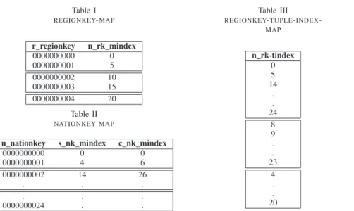
Since two different tables are normally joined by joining primary and foreign key attributes, we create aPK-map(i.e, PrimaryKey map) for each of the primary key in the tables of the star schema. A PK-map will have one column for primary key attribute and one column for each of the foreign keys referencing this primary key as shown in Table Iand

Table II. In the primary key column we store the primary

key attribute values and in the foreign key column we store thelogical record-idof the foreign key. This logical record id runs from 1 to n. The maps are sorted by primary key values, which allows us to apply compression on foreign key logical record-ids and reduce the size of the map to a great extent. Thus, the overall size of the map will be proportional to the number of records in the dimension table (Size of these maps is discussed in Section IV-A)

If there is one projection (partition with one or more columns) of the table sorted by foreign key attribute, then the

Table I REGIONKEY-MAP r regionkey n rk mindex 0000000000 0 0000000001 5 0000000002 10 0000000003 15 0000000004 20 Table II NATIONKEY-MAP

n nationkey s nk mindex c nk mindex

0000000000 0 0 0000000001 4 6 0000000002 14 26 . . . . . . 0000000024 . . Table III

REGIONKEY-TUPLE-INDEX

-MAP n rk-tindex 0 5 14 . . 24 8 9 . . 23 4 . . 20

Note: n rk mindex:n regionkey map index,s nk mindex:s nationkey map index,c nk mindex:c nationkey map index,n rk tindex: n regionkey

tuple index. InTable IIIwe only store the actual record id for logical id 0 to n-1 of second column of Table I

logical record-id of the PK-mapwill be the actual foreign key record-id. Otherwise we need to store the mapping between the logical and actual record-id of the foreign keys. Thus, we create a tuple-index-map as shown in Table III to store these record mapping information.

PK-maps and tuple-index-maps are horizontally

parti-tioned by primary key attribute and distributed to all the nodes containing the corresponding data. Replication of these maps can be done to improve the throughput or disaster recovery. Table I is partitioned into 3 partitions where rows 0 and 1 are assigned to partition 1, rows 2 and 3 to partition 2 and row 4 to partition 3. Accordingly tuple-index-map of foreign keys is partitioned to correspond to the partitions in Table I. Tuple-index-map is partitioned into rows 0 to 9, 10 to 19 and 20 to 24. Similarly, all the other PK-maps and tuple-index-maps are horizontally partitioned.

In the schema of Fig. 1, nation and region tables are very small with only 5 and 25 rows and require less storage space. So, it is not necessary to partition these tables. Instead, these tables can be replicated among all the nodes to improve the performance. But, this may not be the case always. There will be large dimension tables like customer, part or partsupp tables which grow dynamically as new customers and part are added. To show the scenario where all the dimension tables are large and need to be partitioned, we have partitioned the region and nation table.

With this information on PK-maps and tuple-index-mapseach node can execute query independently even when there is a join between two different tables that are located in two different nodes. For example, consider a query:Find

all suppliers of region ”europe”. To find the suppliers we

need to join supplier, nation and region tables of Fig. 1. If these tables are stored among different nodes then we have to communicate with those nodes to get the mapping between the tables. But with our map structures, we can

look up for the mapping and process the query. This reduces the communication among nodes during query execution. In this approach, joins between different tables are done by scanning maps. We will show the detailed processing of some of the TPC-H queries in the coming sections.

With the TPC-H schema of Fig. 1, we need to create

7 PK-maps regionkey-map, nationkey-map, suppkey-map,

partkey-map, partsuppkey-map, custkey-map and orderkey-map. Structure of regionkey-map and nationkey-map are shown in Table 1 and Table 2. Table 1 contains the mapping between regionkeys of region and nation table. Table 2 contains the mapping between nationkeys of nation, supplier and customer tables (Fig. 1). Similarly we can create the remaining 5 maps. Table 3 gives the mapping between logical and actual record-id of the nation table, when the nation table is sorted on nationkey attribute.

In Table 1 and Table 2, first column stores the primary key value and subsequent columns store foreign key logical id (which is the starting id). Since the record-id of primary and foreign keys is same as the map index, we don’t store these values in PK-map and tuple-index-map.

B. Reference Graph

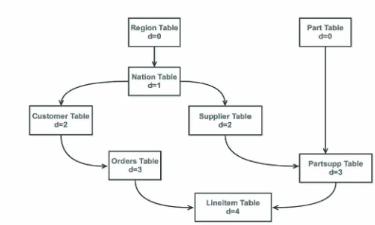
Fig. 2 is the reference graph for the star schema (Fig. 1). Each rectangle box represents a table of the star schema and directed arrows connecting these boxes represent the relationship between the tables. i.e, arrow connecting region table to nation table means the primary key of region table is referred as foreign key in the nation table; d gives the depth of the table, i.e., number of other tables linked to it starting from the table with no reference (d=0).

C. Query Processing Algorithm

With the above PK-maps and reference graph we will design an algorithm to process multi-join queries as shown in Algorithm 1.

Figure 2. Reference Graph for star schema of Fig. 1 Note:”d” is the depth of the table. d=0 means there is no foreign key in current table which refers to primary key of other table. d=1 means there is at least one foreign key in the current table which refers to primary key of other table with d=0.

Input to the algorithm is the query and reference graph, and output of the algorithm is the result of the query. In this algorithm we first retrieve all the tables in the ”from” clause of the query and sort them by the corresponding d value in the reference graph. Then, we process each table predicates starting from the first table of the above sorted order.

Algorithm 1 Query Processing Algorithm

Input: query Q, reference graph G

Output: Result of query Q

1:Let T be an array of tables referenced in Query

2: SortT based ondvalue of G

//d value is shown in Fig. 2

3:for eachtablet∈Tdo

4: ifthere is a predicate on non-PK/non-FKthen

5: ifd == 0 for tthen

6: Apply predicate on t to get the record id’s

7: Store the record-id mapping in the format

8: (rec-id1,rec-id2,.).

9: Communicate if necessary with other nodes

10: else ifany table t1with d1≤d referenced by tthen

11: Apply predicate on t

12: Update the mapping with rec-id’s of t

13: Perform line 9

14: Eliminate mappings which has no match for t

15: else

16: Perform similar to line 6, 9, 14

17: end if

18: else ifthere is a predicate on PK or FKthen

19: ifd == 0 for tthen

20: Scan PK-map and tuple-index map

21: Perform line 6 to 8

22: else

23: Scan PK-map and tuple-index map for those rec-id’s stored for table

t1with d1≤d that is referenced by t

24: Perform 12 and 14

25: end if

26: end if

27:end for

28:Scan tables of T for final mappings(rec-id1,...) to get the values of other attributes

in theselectstatement of Q

29:return Result

Predicates may be to join two tables or to filter records of the table. We store the result of applying predicates in the form (rec-id₁, rec-id₂, rec-id₃,....), where rec-id₁ will

be the record id of first table with d=0 and rec-id₂ will be the record id of the second table which matches the record rec-id₁ and so on. While applying predicate on the tablen,

if we did not find any matching recordn for the previous

result (rec-id1,rec-id2,...rec-idn−1), then we eliminate the

previously stored result(rec-id1,rec-id2,...rec-idn−1). After

processing all the tables, the final result is constructed using the remaining mapping (rec-id₁, rec-id₂, rec-id₃,....) to retrieve non primary and foreign key attribute values of the tables.

Let us look at multi-join query processing by taking some queries of TPC-H benchmark in the next section.

III. CASE STUDY: TPC-H QUERYPROCESSING We randomly chose 3 out of 22 TPC-H queries for analysis which are shown in Fig. 3, Fig. 5 and Fig. 6. In this section we analyze the processing of one of these queries using our approach (section II).

Example 1 in Fig. 3 is a Minimum Cost Supplier Query. The result will display all the suppliers who have minimum supply cost in the region ’EUROPE’ for part size 15 and part type ending with BRASS. The query is processed as shown in the flow diagram in Fig. 4.

This query involves five tables - region, nation, supplier, part and partsupp, four joins between those tables and three predicates on region name (r name), part type (p type) and part size (p size). We can process this query using algorithm 1 as shown below:

T = [ region, part, nation, supplier, partsupp ]

Loop1 Each node will process region table: (executes line 4 to 9 of Algorithm 1)

Scan the region table to get the region key with region name ’EUROPE’ and send the PK-map record-id to all other nodes.

For example, If node 1 finds the regionkey of EU-ROPE as ”0000000003” and its PK-map record-id is 3, then node 1 will send record-id 3 to nodes 2, 3 and 4.

Loop2 Each node will process part table: ( executes line 4 to 9 of Algorithm 1)

Scan the part table to get the partkeys whose p size=15 and p type like ’%BRASS’. Then, send the record-ids of the result to every other node.

Loop3 Each node will process nation table: (executes line 22 to 25 of Algorithm 1)

Scan regionkey-map to get the record-ids of the re-gionkey in the nation table.

Loop4 Each node will process supplier table: (execute line 22 to 25 of Algorithm 1)

Scan nationkey-map to get the logical record-ids of nationkey attribute of supplier table.

Loop5 Each node will process the partsupp table:

Example 1

select s acctbal, s name, n name, p partkey, p mfgr, s address, s phone, s comment

frompart, supplier, partsupp, nation, region

wherep partkey = ps partkey and s suppkey = ps suppkey

and p size = 15 and p type like ’%BRASS’ and s nationkey = n nationkey

and n regionkey = r regionkey and r name = ’EUROPE’ and ps supplycost =(

select min(ps supplycost)

frompartsupp, supplier, nation, region

wherep partkey = ps partkey and s suppkey = ps suppkey and s nationkey = n nationkey and n regionkey = r regionkey and r name = ’EUROPE’)

order by s acctbal desc, n name, s name, p partkey;

Figure 3. TPC-H Query 2 (Source: [9],p. 30)

scan suppkey-map and partkey-map to find the record-ids that are mapped to partsupp table.Then, find the record-ids common to both the results.

For these common record-ids, find the mini-mum ps supplycost. Exchange the local minimini-mum ps supplycost with all other nodes to find the global minimum ps supplycost (line 11 to 14 in algorithm 1) With these results we find the final record-ids.

Final Select all the attribute values required for the final result using the final mapping of the Loop5.

Figure 4. Flow diagram for processing Example 1

Partial results of each of the nodes of the network are then combined to form the final result.

In the Example 1 query processing we need only three communications between the nodes as shown in Loops 1, 2 and 5. But in the general approach, each join of two tables requires communication with other nodes. This is because a node does not know whether there is any record in other node which matches the current node’s record. So communication is needed between nodes after each of the operation like, find the region key for r name ’EUROPE’, join those results with nation table, then join the results with supplier table, find the part keys of part table whose p size 15 and p type like ’%BRASS’, join the results with partsupp table to find the local minimum ps supplycost and then find the final records.

In total, five communications are needed between all participating nodes. So it is clear that usingPK-map struc-ture reduces the communication among the nodes during query processing. Also, in the general approach we need to exchange join attribute values instead of the join indices.

Similarly we can process Example 2 and Example 3 using the Algorithm 1.

IV. STORAGE AND COMMUNICATION MESSAGE SIZE A. PK-map and Tuple-index-map Size

Number of rows of a PK-map is equal to the number of rows of a dimension table (i.e, the primary key table). Number of columns of a PK-map will be equal to the number of foreign keys referencing the primary key plus one (primary key column). Some header information like partition and node information will also be stored to locate the table data stored in different nodes. The overall size of each map will be,

Size of 1st col (S₁) ← (num. of rows of PK) ∗ size of PK

attribute value

Size of other columns (S2)←(num. of rows ofPK) ∗size of record id

i.e, S2←(num. of rows ofPK)∗(size of integer)

SizeOf P KM ap=S1+

n

i=1

S2[i] +c (1)

wherecis the size of the header information,n is the number of foreign keys (FK) referencing primary key (PK) and S₂[i] is the size of the column of the foreign key i.

Size of thetuple-index-map will be equal to the size of integer times the number of rows of the foreign key table. SizeOf T upleIndexM ap= (num.Of RowsOf F K)∗(sizeOf Int)

Example 2

select n name, sum(l extendedprice *(1 - l discount)) as revenue

fromcustomer, orders, lineitem,supplier, nation, region

wherec custkey = o custkey and l orderkey = o orderkey and l suppkey = s suppkey and c nationkey = s nationkey and s nationkey = n nationkey and n regionkey = r regionkey and r name = ’ASIA’

and o orderdate>= date ’1994-01-01’

and o orderdate<date ’1994-01-01’ + interval ’1’ year

group by n name

order by revenue desc;

Figure 5. TPC-H Query 5 (Source: [9], p.37)

Example 3

selectc custkey, c name,

sum(l extendedprice*(1-l discount)) as revenue, c acctbal, n name, c address, c phone, c comment

fromcustomer, orders, lineitem, nation

wherec custkey = o custkey and l orderkey = o orderkey

and o orderdate>= date ’1993-10-01’

and o orderdate<date ’1993-10-01’ + interval ’3’ month and l returnflag = ’R’

and c nationkey = n nationkey

group byc custkey, c name, c acctbal, c phone, n name, c address, c comment

order byrevenue desc;

Figure 6. TPC-H Query 10 (Source: [9], p.46)

For example, consider 5 regions and 25 nations (each region has 5 nations). PK-maps: regionkey-map and nationkey-map will look like Table I and Table II. Tuple-index-map: regionkey-tuple-index-map will look like Table III. Let us consider the size of region key be varchar(10) and nation key be varchar(10).

Table I size: S₁ = 50 bytes, S₂ = 40 bytes and Size of regionkey-map is 90 + c ≈90 bytes

Table II size: S₁ = 250 bytes, S₂ = 200 bytes and Size of nationkey-map is, 650 + c ≈650 bytes

Table III size: Number of rows of nation table is 25. Size of regionkey-tuple-index-map is, 25 * 4 = 100 bytes

Similarly we can calculate the size of the remaining maps and find the total storage space needed to store all the required maps. We will show the total size of all the required maps for 10GB of data in Section V.

Size of PK-map will always be small because the di-mension table will always be smaller than the fact table and dimension table will grow slower than the fact table. PK-map will grow only when the new primary key is added to the dimension table. When a new row is added to fact table, we just have to update the value in the PK-map

and append a row to the tuple-index-map. Tuple-index-map grows proportionally to the fact table.

B. Inter-node Communication Message Size

Inter-node communication message size is the size of the intermediate query result sent from one node to another. Pro-cessing the query (Fig. 3), using our approach requires only 3 communications whereas the general approach requires 5 communications. In our approach, nodes exchange only map indices but in the general approach nodes exchange much larger join attribute values . Thus reducing the size of the inter-node communication overhead.

For example, as shown in Section III, using our approach nodes communicate only record-ids during the execution of Example 1 query. First, record-id of EUROPE region is communicated. So, the message size is 4 + c bytes, where 4 is the size of record-id (integer) and c accounts for header information. In general approach the message size will be (10*4)+c bytes, where 10 is the size of region key attribute (varchar). In this case the message size is small, but when results of large tables need to be exchanged the message size will be significantly larger.

We will show the total size of the intermediate results exchanged during the execution of query in the next section.

V. PERFORMANCEEVALUATION

Our test environment is a network of four virtual CentOS machines. Each of these machines has 2.6GHz Six-Core AMD Opteron Processor, 2GB RAM and 10GB disk space. Also, these machines have Oracle 11g.

For experiments we generated data using data generator

dbgen provided by TPC-H benchmark and distributed it to all four nodes. We generated 10GB of data for the experiments in Section 5.2 to 5.4. We generated PK-maps and tuple-index-maps, and horizontally partitioned them into four partitions and distributed them to the four nodes. We used same partition keys to partition the data and to compare performance between our and general approach. We took same three queries which we have analyzed in Section III to analyze the performance.

Due to the time constraint we were unable to show the results of our performance analysis on a commercial cloud. Since we were able to achieve significant performance improvement using four virtual nodes, we can say that the experiments are proofs of concept on the saving of communication costs for query execution. In a large cloud environment, the communication cost has a even greater weight in query costs [23] [24]. Therefore, the savings resulted from our work would be even more significant.

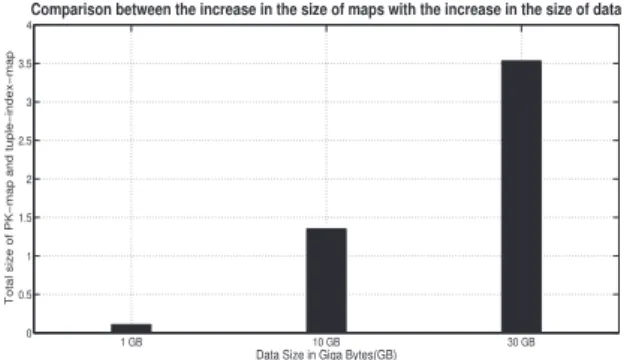
1 GB 10 GB 30 GB 0 0.5 1 1.5 2 2.5 3 3.5 4

Data Size in Giga Bytes(GB)

Total size of PK−map and tuple−index−map

Comparison between the increase in the size of maps with the increase in the size of data

Figure 7. Comparison between increase in the size of PK-map and tuple-index-map with the increase in the size of data

Example 1 Example 2 Example 3 0 5 10 15 20 25 30 35 40 45 50

Example queries of Fig. 2, Fig. 3 and Fig. 4

Message size in MB

Comparison of total size of messages sent between nodes during the execution of example queries

our approach general method

Figure 8. Comparison of total size of inter-node communication while processing queries using our approach and with general approach

Example 1 Example 2 Example 3 0 100 200 300 400 500 600 700 800

Query execution of examples 1, 2 and 3

Time taken in seconds

Comparison of execution time of example queries using our approach and general method

our approach general method

Figure 9. Comparison of execution time of queries using our approach and with general approach

Example 1 Example 2 Example 3 0

5 10 15

Queries of Fig. 2, Fig. 3 and Fig. 4

Number of communication

Comparison of the number of communications between nodes executing query

Our approach General approach

Figure 10. Comparison of number of communications while executing queries using our approach and with general approach

A. Size of PK-maps and Tuple-index-maps

To show that the size of our PK-maps and tuple-index-maps grow linearly with the data size, we generated 1GB, 10GB and 30GB data using dbgen and then created PK-maps and tuple-index-PK-maps for each of these data. Size of these maps are shown in Fig. 7.

We observe from Fig. 7 that, total size of map structures will be around 10% to 12% of the data size. These maps will then be partitioned and distributed to all nodes.

B. Size of Inter-node Communication Messages

To compare the inter-node communication message size between the proposed and general approach, we added the size of all the messages exchanged while executing the queries. The comparison results are shown in Fig. 8.

In the graph (Fig 8), queries are on the x-axis and the total message size in MB (Mega Bytes) on the y-axis. On x-axis, for each query we have 2 bars, where first bar (in black)shows the total size of the messages used in our approach and the second bar (in white) shows the total size of the messages used in general approach.

As we can see in the graph (Fig. 8), execution of Example 1 query exchange 0.5MB of data in our approach and 1.1MB of data in the general approach. Execution of Example 2 query involves exchange of 12MB of data in our approach and 20MB in general approach. Execution of Example 3

query involves exchange of 15 MB of data in our approach and 48MB in general approach.

Based on the result in Fig. 8, the total communicated message size is much less with our approach than that of the general approach.

C. Multi-join Query Execution

Comparison of execution time of joins of queries in Fig. 3, Fig. 5 and Fig. 6 are shown in Fig. 9. In this graph(Fig. 9), queries are on the x-axis and execution time (in seconds) on the y-axis. On x-axis, for each query we have 2 bars, where first bar (in black) shows the time taken by our approach and the second bar (in white) shows the time taken with the general approach.

As we can see from this graph (Fig. 9), Example 1 query takes 63 seconds to run in our approach and 235 seconds in general approach. Example 2 query takes 206 seconds in our approach and 741 seconds in general approach. Example 3 query takes 125 seconds in our approach and 712 seconds in general approach.

Based on the data in Fig. 9, we can infer that query execution is faster with our approach than with general approach.

D. Number of Inter-node Communications

As each inter-node communication has some inherent overhead, we also compare the number of messages in

addition to the message size.

Comparisons on the total number of messages exchanged during the execution queries are shown in Fig. 10. In this graph (Fig. 10), queries are on the x-axis and the number of messages are on the y-axis. Example 1 query execution involves nine communications (i.e, 3 times communication with 3 nodes) using our approach and fifteen communi-cations in general approach. Example 2 query execution involves six communications in our approach and fifteen communications in general approach. Example 3 query execution involves three communications with our approach and nine communications in general approach.

Based on the result in Fig. 10, we can infer that the number of communications in our approach is fewer than in the general approach. This optimization has a big impact, since the number of communications increases rapidly with increase in number of nodes.

VI. ACKNOWLEDGMENTS

Tingjian Ge is supported in part by the NSF, under the grants IIS-1149417 and IIS-1239176. Benyuan Liu is supported by NSF grant CNS-0953620.

VII. CONCLUSION

In this paper, we proposed storage structures PK-map and tuple-index-map. PK-map stores mapping information of primary and foreign keys, and tuple index-map stores the mapping of logical to actual record-ids of foreign keys. We then designed an algorithm for processing multi-join queries using the proposed storage structures. We presented an empirical study of our proposed approach using some of the queries of TPCH benchmark. Results demonstrate that the proposed approach improves the performance of the ad-hoc multi-join query in cloud environment and reduces communication overhead. REFERENCES [1] AmazonEC2: http://aws.amazon.com/ec2/ [2] GoogleCloud: http://www.google.com/enterprise/cloud/storage/ [3] Greenplum,EMC: http://www.greenplum.com/products/greenplum-database [4] IBM: http://www-01.ibm.com/software/data/infosphere/warehouse/ [5] Microsoft:http://msdn.microsoft.com/enus/library/aa197903 (v=sql.80).aspx [6] Microstrategy: http://www.microstrategy.com/ [7] OracleBI:http://www.oracle.com/us/solutions/ent-performancebi/enterprise-edition-066546.html [8] SqlServer: http://technet.microsoft.com/enus/sqlserver/cc510300.aspx [9] TPC-H: http://www.tpc.org/tpch/spec/tpch2.14.4.pdf. [10] Vertica:http://184.106.12.19/wp-content/uploads/2011/01/VerticaArchitectureWhitePaper.pdf [11] D. J. Abadi. Data management in the cloud: Limitations and

opportunities. IEEE Data Eng. Bulletin ’09, Volume 32(1):3-12

[12] D. J. Abadi, P. A. Boncz, and S. Harizopoulos. Column-oriented database systems. In Proceeding, VLDB ’09, 2(2):1664-1665.

[13] D. J. Abadi, S. R. Madden, and N. Hachem.Column-stores vs. row-stores: how different are they really?In Proceeding, ACM SIGMOD ’08, pages 967-980, New York, NY, USA. [14] A. Abouzeid, K. Bajda-Pawlikowski, D. Abadi, A.

Silber-schatz, and A. Rasin.Hadoopdb: an architectural hybrid of mapreduce and dbms technologies for analytical workloads. In Proceeding, VLDB ’09, 2(1):922-933.

[15] M. O. Akinde, M. H. Bohlen,T. Johnson, L. V. Lakshmanan, and D. Srivastava. efficient olap query processing in dis-tributed data warehouses, 2002.

[16] G. Candea, N. Polyzotis, and R. Vingralek.A scalable, pre-dictable join operator for highly concurrent data warehouses. In Proceeding, VLDB ’09, 2(1):277-288.

[17] A. L. Holloway and D. J. DeWitt.Read-optimized databases, in depth.In Proceeding, VLDB ’08, 1(1):502-513.

[18] M. Ivanova, M. L. Kersten, and N. Nes. Self-organizing strategies for a column-store database.In Proceeding, EDBT ’08, pages 157-168, New York, NY, USA.

[19] R. MacNicol and B. French. Sybase iq multiplex designed for analytics.In Proceeding, VLDB ’04, pages 1227-1230. [20] D. P. Panos Kalnis.Multi-query optimization for on-line

ana-lytical processing.. In Journal, Information Systems, Volume 28 Issue 5, July 2003.

[21] M. Stonebraker, D. J. Abadi, A. Batkin, X. Chen, M. Cher-niack, M. Ferreira, E. Lau, A. Lin, S. Madden, E. O’Neil, P. O’Neil, A. Rasin, N. Tran, and S. Zdonik. C-store: a column-oriented dbms. In Proceeding, VLDB ’05, pages 553-564. [22] H. Wang, X. Meng, and Y. Chai. Efficient data distribution

strategy for join query processing in the cloud.In Proceeding, CloudDB ’11, pages 15-22, New York, NY, USA.

[23] Waqar Hasan, Rajeev Motwani. Optimization Algorithms for Exploiting the Parallelism-Communication Tradeoff in Pipelined Parallelism. In Proceeding, VLDB ’94, Santiago de Chile, Chile.

[24] Jian Li, Amol Deshpande, Samir Khuller.Minimizing Com-munication Cost in Distributed Multi-query Processing. In Proceeding, ICDE ’09, Shanghai, China.