On the Distribution of Crop Yields: Does the Central Limit Theorem Apply?

On the Distribution of Crop Yields: Does the

Central Limit Theorem Apply?

Abstract

In this paper we take issue with the applicability of the central limit theorem (CLT) on aggregate crop yields. We argue that even after correcting for the e¤ects of spatial de-pendence, systemic heterogeneities and risk factors, aggregation does not necessarily lead to normality. We show that aggregation is also likely to lead to nonnormal distributions, which exhibit both skewness and excess kurtosis. In particular, we consider the case in which the number of summands is not constant but varies with time, which corresponds to the empirically relevant situation where the number of acres used for cultivation of a particular crop exhibits substantial variation over time. In this case, the CLT is not applicable while the limit theorems for random sums of random variables, which apply, predict that the limiting distribution of the sum is not normal and depends on the pos-tulated distribution of the number of summands. Using data from aggregate US states crop yields, we provide empirical support regarding the deviation of aggregate crops yields from normality.

JEL Classi…cation: C16, C51, Q14

Keywords: Aggregate Crop Yield; Central Limit Theorem; Limit Theorem for Random Sums of Random Variables; Normality.

The probability distribution of crop yields has been extensively investigated over the last twenty years or so; however its characterization still remains an open is-sue. Several authors, such as Just and Weninger (1999), Ker and Goodwin (2000), Atwood, Shaik and Whatts (2002, 2003), Sherrick et al. (2004), Hennessy (2009), to name a few of the recent contributors to this literature, focus on the question of whether crop yields deviate from normality.

Just and Weninger (1999) identify the following reasons, which are likely to pre-vent the emergence of a general consensus on the shape of crop yield distribution: (i) The lack of a clear pattern against normality. In spite of the presence of ample empirical evidence against normality, the origins of the latter are not at all clear. For example, in an early study, Day (1965) reports weak evidence for positive skeweness and nonnormal kurtosis (both leptokurtosis and platykurtosis) for Mississipi cotton, corn and oats yields. Using aggregate time series data, Gallagher (1987) …nds neg-ative skewness in US soybean yields, a result consistent with Taylor (1990). The latter study, however, reports evidence on positive skewness for the wheat yields together with leptokurtosis for all crops (corn soybean and wheat) under consid-eration (see also Buccola 1986, Moss and Shonkwiler 1993). (ii) The uncertainty surrounding the speci…cation of the conditional mean and conditional variance of yields. Misspeci…cation of the systematic components of crop yields are likely to introduce nonstationarity in the random component thus producing erroneous in-ferences on the distributional properties of the latter. In the same spirit, Hennessy (2009, p. 46) noted that “...when systemic heterogeneities exist in the data under consideration, these will dominate to determine the shape of the yield distribution”. He also provided a link between the skewness of aggregate yield and the weather fac-tor skewness. (iii) Misinterpretation of statistical signi…cance. This problem arises in a univariate framework when one fails to combine the various tests for normality

The same problem is also likely to arise in a multivariate framework, if the possible correlations among yields of several crops are ignored. (iv) The use of aggregate time series (ATS) data to represent farm-speci…c variation. At each point in time, crop yield data are constructed by taking the acreage-weighted average over the sample farms. This averaging operation eliminates the speci…c probabilistic features of the yields of each individual farm, thus obscuring the production uncertainty characteristics at the farm-level.

All issues raised above are indeed valid. However, Just and Weninger make an additional point concerning the necessity of the normal distribution as the appropri-ate probabilistic description of crop yields, which arises from the fact that the CLT seems to be at work. Speci…cally, Just and Weninger correctly point out that “crop yields at all levels are averages”. In particular, they state: “At the aggregate level, ATS data are averages of yields over many farms. At the farm-level, yields are av-erages of production over many acres”(pp. 301). As a result, the above mentioned authors conclude that “under broad conditions”the probability distribution of these averages has to be the normal because of the CLT. On the other hand, Goodwin and Ker (1998) and Goodwin and Mahul (2004), among others, state that the exis-tence of spatial dependence and systemic risk factors indicate that a straightforward application of the CLT is not appropriate.

In this paper we take issue with the applicability of the CLT on aggregate crop yields, arguing that even after correcting for the e¤ects of spatial dependence, sys-temic heterogeneities and (syssys-temic) risk factors, aggregation does not necessarily lead to normality but instead it is also likely to lead to nonnormal distributions, which exhibit both skewness and excess kurtosis. Put it di¤erently, although we do accept the fact that crop yields are indeed averages and also that “convergence in distribution” seems to be in place (in the sense that no distributional explosion is observed) we do not accept that the only possible limiting distribution is the

nor-mal. More speci…cally, we consider the case in which the number of summands is not constant but varies with time, being a random variable itself. This corresponds to the case in which the number of acres used for the cultivation of a particular crop exhibits substantial variation over time. Indeed, one of the most critical decisions that a farmer makes is what crops to grow on the land she has available. For some farmers, the decision of which crops to cultivate is straight forward because the land, climate, tradition, infrastructure and economic conditions all support one dominant crop1_{. However, these farmers still need to decide each year how many acres of}

this crop they will cultivate, which may be a function of unpredictable economic conditions. For other farmers, there may be a variety of crops adapted to their local ecology, and they may wrestle each year with the decision of what crops to plant on what pieces of land. Factors that can a¤ect cropping decisions in a random way are predictions about the weather and predictions on what crops may be planted in other parts of the country or the world which will in‡uence expectations about prices for di¤erent crops at the end of the growing season.

Under this set of assumptions, the central limit theorem is not applicable; in-stead we must appeal to limit theorems for random sums of random variables (see Gnedenko and Korolev 1996). These theorems predict that the limiting distribution of the sum is not normal and depends on the postulated distribution for the number of summands (see Clark 1973 and Blattberg and Gonedes 1974, among others, for an application of these ideas to stock returns). Using data from US aggregate state crop yields, we provide empirical support for the predictions of these theorems. In particular, we …nd positive correlation between crop-speci…c acreage and a set of statistics that measure the deviation of aggregate crops yield from normality.

This paper is organized as follows: …rst, the case against standard convergence to normality mentioned above is analyzed in detail, then the relevant empirical support

On the Applicability of the Central Limit Theorem: The case

of Random Sums

As mentioned in Introduction, Just and Weninger (1999) make a case for the nor-mality of the distribution of crop yields by appealing to the CLT. More speci…cally, they claim that “At the aggregate level ATS data are averages of yields over many farms. At the farm-level, yields are averages of production over many acres. The CLT implies that averages have asymptotically normal distributions under broad conditions” (Just and Weninger 1999, pp 301). Let us formalize this statement. First, we may assume that the random variable of interest is the production of a speci…c acre, with corresponding indexj; at time t, denoted by jt. Obviously, the

values of the random variable _jt (that is the production of each speci…c acre j at time t) are not observable. Nevertheless, what is observable is the production at the State, county, or even farm level as well as the total acreage of each State (or county or farm) devoted to the production of a speci…c crop. So, letXit and nit be

the production and the acreage of farm i, respectively, kt be the number of farms

and Nt= kt P

i=1

nit be the total acreage of all farms at time t. Then, the average yield

per acre is given by:

y_t= kt P i=1 Xit kt P i=1 nit = Nt P j=1 jt Nt (1)

More speci…cally, we must distinguish between the probabilistic properties of the

jt’s within the same time period t (cross-sectional properties) and those across

time (temporal properties). To formalize this, we may arrange the random variables

t= 1 t= 2 ::: j = 1 _{11 12} ::: j = 2 _{21 22} ::: : : : j =Nt N11 N22 ::: (2)

where the last line in (2) does not correspond to a speci…c row but it describes the last element of each column.

In this general setting, the random variables _jt may be characterised by two types of dependence. The …rst one is cross-sectional dependence, that is dependence among the elements of the columns of (2). The second is temporal dependence among the elements of the rows of (2). Put it di¤erently, cross sectional dependence refers to dependence among the crop yields of various acres within the same time period, whereas temporal dependence concerns the dependence among jts across

di¤erent time periods. Similar distinctions can be made about time and spatial heterogeneity. More speci…cally, cross-sectional heterogeneity concerns the extent to which the distributions, D( ); of the yields of various acres within the same period are di¤erent, whereas time heterogeneity refers to the distributions of the total yield across di¤erent time periods. For example, if D( ₁₁) = D( ₂₁) = ::: = D( _N11) then we have cross-sectional homogeneity for t= 1: On the other hand, if D(y₁) =

D(y₂) =::: then the distributions of the average yield over time are identical:

Let t and t denote the mean and standard deviation of jt at time t. In

other words, we assume that the …rst two moments of _jt are equal across j = 1;2; :::; Nt (cross-sectional homogeneity of the second-order). The CLT states that,

under some additional conditions on the probabilistic properties of the individual random variables _jt; p Nt(yt t) t L !N(0;1): (3)

As an implication of (3), we have that for largeNt;

y_{t '}N( _t; 2_t=Nt) (4)

Remarks

(i) Just and Weninger claim that the (cross-sectional) conditions under which (4) is true, are “broad”. Indeed, recent results in Probability Theory on the con-ditions under which CLT applies seem to make a very strong case in favor of the approximate normality of y_t. More speci…cally, it has been proved that CLT holds under quite general properties for the initial sequence _{f jtg}j 1 (with …xed t): For

example, Ibragimov (1962) proves that _{f jtg}j 1 obeys CLT if it is strictly

station-ary, mixing sequence with E_{j 1tj}2+ t

< ₁; for some t > 0: Herrndorf (1984)

relaxes the assumption of stationarity and derives a CLT for mixing sequences of random variables satisfying the condition sup_i2NE_{j itj}bt

< ₁; for some bt > 2

(see Kourogenis and Pittis 2009 for a survey of CLT’s). On the contrary, when the area under consideration is restricted, then spatial dependence may not dissipate fast enough for CLT to hold (see Goodwin and Ker (1998), Goodwin and Mahul (2004) among others).

(ii) It is obvious from (4) that a su¢ cient condition for achieving time homo-geneity amounts to t= and t= 2 >0 for every t.

One of the assumptions implicit in (4) is that the number, Nt, of summands is

large and “certain”. In many interesting cases, however, the number of the sum-mands is not constant but is itself a random variable. In such cases, it is interesting to investigate the limiting behaviour of the so-called “random sums”of random vari-ables. More speci…cally, we are interested in …nding the conditions (if any) under whichN(0;1)is still a good approximation of the distribution of the aggregate crop yields, if the number,Nt(the total acreage) of the jt’s (production per acre) is large

but random. Put it di¤erently, we are interested in examining whether there are any conditions under which, for each t, the jt’s may still belong to the domain of

attraction of the normal law, even in the presence of randomness in the number of summands. We are also interested in identifying the cases for which a distribution,

D;di¤erent thanN(0;1)is the appropriate limiting distribution of the random sum and studying its properties.

To de…ne the problem, for each t, let _f jgi 1 be an iid sequence of random

variables with …niteE( _j) = and V ar( _j) = 2 _{>0. Obviously, the moments}

and 2 may in general vary across time, but since the analysis that follows refers to a speci…c time period, we choose to drop the second subscript t from the more appropriate notation

t and

2

t for simplicity. Moreover, (and following the same notational convention of dropping the time subscript) let_fNngn 1 be a sequence of

nonnegative integer-valued random variables. De…ne the random sum process

SNn =

Nn X

i=1

j:

The question to be answered is under what conditions the random sum, SNn; prop-erly normed and centered, converges in law to some random variable,Z;and further, under what additional conditionsZ is distributed asN(0;1):Robbins (1948) obtains su¢ cient conditions for the convergence in law of the properly centered and normed sequenceSNn; to normal, under the assumption thatNn is independent of the sum-mands, 1, 2; :::. Renyi (1960) and Blum, Hanson and Rosenblatt (1963) derive

su¢ cient conditions similar to those of Robbins (1948) without the assumption of independence betweenNn and the summands.

ran-dom sum process, Zn; as follows:

Zn =

SNn n q

n 2

We are interested in …nding the general conditions under which the sequence of theZn’s converges in law to a random variable Z; as well as the speci…c conditions

guaranteeing that Z N(0;1): Finkelstein and Tucker (1989) show that under the assumption that Nn is independent of the summands, the necessary and su¢ cient

condition for Zn L ! (some) Z (5) is given by Un Nn n p n L ! (some)U: (6)

In such a case, the distribution of Z is that of the sum of two independent random variables, Z1 and Z2; where Z1 is N(0;1) and the distribution of Z2 is the same

to that of U: This result may be stated in an equivalent way by saying that the distribution functionFZ ofZ is equal to FU where andFU are the distribution

functions of the standard normal andU, respectively. In other words,Z is a mixture of normals, with the mean being mixed by U (see Finkelstein, Kruglov and Tucker 1994).

Finkelstein and Tucker (1989) also derive the conditions for the convergence of

Zn to N(0;1): Speci…cally, they show that if (and only if) condition (6) is replaced

by Un Nn n p_n !p 0; (7) then Zn L ! N(0;1): (8)

Remarks:

(i) Condition (7) is stronger than (6). This in turn implies that the assump-tions that must be made on the behavior of_fNngn 1 in order to obtain asymptotic

normality are stronger than the ones that ensure simply convergence to some dis-tribution. In the case that (6) holds but (7) fails, the sequenceZn of random sums

converges in law to a non-normal random variable, which is likely to exhibit both skewness and excess kurtosis.

(ii) The case analyzed above is usually referred to as “convergence of random sums under nonrandom centering”. This is due to the fact that the random sum process SNn is centered by the sequence of constants, n . A somewhat di¤erent problem arises in the case that the sequence SNn is centered by Nn instead of

n : In such a case, the random sum process is centered by a sequence of random variables rather than by a sequence of constants. This asymptotic problem, referred to as “convergence of random sums under random centering” was …rst analyzed by Renyi (1960) who showed that the centered and normed random sum process,

Z_n SNn Nn xpn (9) converges to N(0;1)if Nn n p !1: (10)

Condition (10) which ensures convergence toN(0;1)in the case of random centering is weaker and hence easier to be satis…ed in practice than (7) which corresponds to the case of nonrandom centering. However, nonrandom centering is more natural for constructing approximate distributions. Moreover, Korolev (1995) argues that random centering “signi…cantly restricts the class of possible limit laws compared to the general situation, where random sums are centered by constants” (1995, pp.

(ii) The results analyzed above were obtained under the restrictive assumption that the initial random variables, j; are iid with …nite mean, ; and variance,

2_{. Billingsley (1962) extends this result by proving the asymptotic normality of}

Z_n for the cases in which (10) holds and the initial sequence _{f jg}i 1 obeys the

“invariance principle” (IP). The latter is a stronger version of the classical central limit theorem for nonrandom partial sums. It has been shown that IP is satis…ed by a wide spectrum of non iid sequences _f jgi 1; such as strong or uniform mixing

ones (see Kourogenis and Pittis 2009 for a recent survey on this topic). This result implies that Z_{n !}L N(0;1) holds under (10) even for cases in which _f jgi 1 is an

asymptotically independent, nonstationary sequence.

The practical implications of the preceding discussion may be summarized as follows:

(i) When a random variable,Z; is the sum of elementary random variables, then its distribution may be approximated by the normal one, even if the number of summands, Nn; is random. This is valid when Nn behaves in a way prescribed by

conditions (7) or (10). Speci…cally, Nn must exhibit small variation around n for

large n. If Nn displays considerable variability around n even for large n; then the

asymptotic distribution ofZ is not normal but rather a mixture of normals. In such a case, the empirical distribution ofZ is likely to exhibit both skewness and excess kurtosis.

(ii) In assessing the distribution of crop yields using aggregate time series data, we face the following problems: First we must account for possible trends in the aggregate series arising from time heterogeneity in the moments of the j’s. More

speci…cally, if we assume that E( _jt) = t then the aggregate crop yield series will exhibit a trending behavior, which has to be accounted for before any tests for normality are carried out. This issue is analyzed in the third and fourth sections of Just and Weninger (1999) and is also considered in the empirical section of this

paper. However, even if we succeed in correctly detrending the aggregate series, we still face the problem of the possible variation (randomness) of the number of acres that enter the calculation of the aggregate yield over time. If this variation is substantial (in the sense that it violates conditions (7) or (10)), then non-normality of the aggregate data is likely to arise.

Verbally, we consider the case in which the number of summands is not constant but varies with time, being a random variable itself. This corresponds to the case in which the number of acres used for the cultivation of a particular crop exhibits substantial variation over time and this variation is more or less random. As dis-cussed in Introduction, factors that can a¤ect cropping decisions in a random way are predictions about the weather and predictions on what crops may be planted in other parts of the country or the world which will in‡uence expectations about prices for di¤erent crops at the end of the growing season.

Empirical Results

The analysis of the previous section suggests that the presence of non-normality in the crop yield distributions is likely to derive from the random nature of the number of acres employed in the production of various crops over time. This assumption implies that we should observe some signi…cant correlation between the sample stan-dard deviation, s( Nt); of the percent annual changes, Nt; of the total number

of acres employed in the production of a speci…c crop and any measure of non-normality (such as skeweness and excess kurtosis coe¢ cients) of the distribution of the aggregate (State level) yield of this crop. To examine this empirical implication, we …rst estimate the skeweness, 3; and kurtosis, 4, coe¢ cients of the distribution

of percent annual changes, yt; of the yields of …ve major crops, namely cotton,

the residuals, ut, of an auxiliary autoregression of yt on yt 1, yt 2 and a time

trend. The latter case aims at controlling for non-normality e¤ects caused by the presence of temporal dependence and/or time heterogeneity (deterministic or sto-chastic) in the original crop yield series (see Just and Weninger 1999 for a detailed discussion of these points).

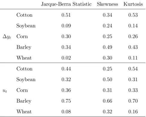
Table 1 around here

Table 1 reports the following correlation coe¢ cients: (i) the correlation between

s( Nt) and the absolute value of 3; (ii) the correlation between s( Nt) and the

absolute value of 4 3; (iii) the correlation between s( Nt) and JB. Note that

the employed distributional characteristics have been calculated for two alterna-tive empirical distributions of crop yields. The …rst one refers to the raw data of

yt whereas the second one corresponds to the residuals ut. The results may be

summarized as follows:

(i) All estimated correlation coe¢ cients have positive sign thus suggesting a pos-itive relationship between the standard deviation of Nt and each of the employed

measures of non-normality.

(ii) The magnitude of these correlation coe¢ cients, in general, seems to be higher for the case in which the detrended and demeaned crop yield series are employed. For example, for the case of soybean, the correlation coe¢ cient between s( Nt)

and _j 3j is equal to 0.24 and 0.50 for the cases of raw and …ltered crop yield series

respectively.

(iii) In some cases, the estimated correlation coe¢ cients exceed the value of 0.5, thus reaching an impressively high value. For example, the correlation coe¢ cient betweens( Nt)and j 4 3jfor the case of the …ltered cotton yield is equal to 0.54,

whereas the same coe¢ cient for the case of …ltered barley yield reaches the value of 0.70.

(iv) When the residuals ut are employed, the smallest correlation coe¢ cient is

the one betweens( Nt)and the Jarque-Berra Statistic for the case of wheat and is

equal to 0.08. It is interesting to note that this is the crop for which Nt exhibits

the smallest average variation across States. More speci…cally, the mean of the estimated s( Nt)’s across States is equal to 30.71, 36.22, 25.40, 34.35 and 25.1 for

cotton, soybean, corn, barley and wheat, respectively. This piece of evidence implies that the minimum “correlation e¤ects” appear in the case of wheat for which the percent annual changes of the total number of acres displays the minimum variation among the …ve crops under consideration.

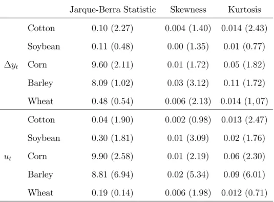
Table 2 reports the estimated regression coe¢ cients and the corresponding t -statistics between the standard deviation of Nt (explanatory variable) and the the

distributional characteristics of crop yield changes, as measured by the skeweness, the kurtosis and the Jarque-Berra Statistic:

Table 2 around here

In accordance with the results of Table 1, we …nd that when the statistics of the residuals ut are used, all crops have at least one regression coe¢ cient with

corre-spondingt-statistic greater than 1.96. More speci…cally:

(i) The higher values of the t-statistics correspond to barley (all greater than 5) and to corn (all greater than 2.1).

(ii) The absolute values of thet-statistics whenuts are used are in general higher

than the corresponding ones for the case where yts are employed.

Conclusions

distri-of the CLT. We argue that normality is not an inevitable consequence distri-of the op-eration of aggregation of crop yields. Motivated by the empirical observation that the number of crop-speci…c acres exhibits substantial variation over time (due to weather predictions or predictions about cultivation decisions elsewhere that will a¤ect expectations on crop prices), we consider limit theorems that are applicable when the number of summands is not constant but varies with time. These theorems predict that the limiting distribution of the sum is not normal and depends on the postulated distribution for the number of summands.

Our empirical analysis investigates the existence of signi…cant correlation be-tween the sample standard deviation of the percent annual changes of the total number of acres employed in the production of a speci…c crop ( Nt) and di¤erent

measures of non-normality (skeweness and excess kurtosis coe¢ cients) of the distri-bution of the aggregate yield of this crop. We apply this investigation to …ve major crops, namely cotton, soybean, corn, barely and wheat. To hedge against the pres-ence of non-normality e¤ects due to temporal dependpres-ence and/or time heterogeneity in the original crop yield series, we apply the same investigation to the de-trended and demeaned series of the same crops. Our results provide empirical support for our theoretical predictions. In particular, we …nd a positive relationship between

Nt and di¤erent measures of non-normality, the magnitude of which increases,

reaching impressively high values for some crops, when we use the de-trended and demeaned crop series.

Our results have implications for the correct speci…cation and estimation of econometric models of crop yields, since we have identi…ed an additional factor, namely the standard deviation of Nt, which can cause nonzero skewness and

ex-cess kurtosis in the distribution of aggregate crop yields. This implies that when policy-making is based on these estimated models, one needs to be cautious to take into account the changes in crop-speci…c acreage, in order to avoid unreliable and

misleading results deriving from distributional mispeci…cation.

References

[1]Atwood, J., Shaik, S., Watts, M. (2002). Can Normality of Yields Be Assumed for Crop Insurance? Canadian Journal of Agricultural Economics 50, 171-184. [2]Atwood, J., Shaik, S., Watts, M. (2003). Are Crop Yields Normally Distributed?

A Reexamination.American Journal of Agricultural Economics 85, 888-901. [3]Billingsley, P. (1962). Limit Theorems for Randomly Selected Partial Sums.

An-nals of Mathematical Statistics 33, 85-92.

[4]Blattberg, R. C., Gonedes, N. J. (1974). A Comparison of the Stable and Student Distributions as Statistical Models for Stock Prices.Journal of Business 47, 244-280.

[5]Blum, J. R., Hanson, D. L., Rosenblatt, J. I. (1963). On the central limit theorem for the sum of a random number of independent random variables. Probability Theory and Related Fields 1, 389-393.

[6]Buccola, S. T. (1986). Testing for Nonnormality in Farm Net Returns. American Journal of Agricultural Economics 68,. 334-343.

[7]Clark, P. K. (1973). A Subordinated Stochastic Process Model with Finite Vari-ance for Speculative Prices. Econometrica 41, 135-155.

[8]Day, R. H. (1965). Probability Distributions of Field Crop Yields. Journal of Farm Economics 47, 713-741.

[9]Finkelstein M., Tucker, H. G. (1989). A Necessary and Su¢ cient Condition for Convergence in Law of Random Sums of Random Variables Under Nonrandom Centering.Proceedings of the American Mathematical Society 107, 1061-1070. [10]Finkelstein, M., Kruglov, V. M., Tucker, H. G. (1994). Convergence in law of

random sums with non-random centering. Journal of Theoretical Probability 7, 565-598.

[11]Gallagher, P. (1987). U.S. Soybean Yields: Estimation and Forecasting with Nonsymmetric Disturbances. American Journal of Agricultural Economics 69, 796-803.

[12]Gnedenko, B. V., Korolev, V. Y. (1996). Random summation: limit theorems and applications. CRC Press LCC, Boca Raton, Florida.

[14]Hennessy, D. A. (2009). Crop Yield Skewness and the Normal Distribution. Jour-nal of Agricultural and Resource Economics 34, 34-52.

[15]Herrndorf, N. (1984). A functional central limit theorem for weakly dependent sequences of random variables. Annals of Probability 12, 141-153.

[16]Ibragimov, I. A. (1962). Some limit theorems for stationary processes. Theory Prob. Appl. 7, 349-382.

[17]Just, R. E., Weninger, Q. (1999). Are Crop Yields Normally Distributed? Amer-ican Journal of Agricultural Economics 81, 287-304.

[18]Ker, A. P., Goodwin, B. K. (2000). Nonparametric Estimation of Crop Insurance Rates Revisited. American Journal of Agricultural Economics 82, 463-478. [19]Kourogenis, N., Pittis, N. (forthcoming). “Mixing Conditions, Central Limit

Theorems and Invariance Principles: A Survey of the Literature with Some New Results on Heteroscedastic Sequences”, Econometric Reviews.

[20]Korolev, V. Y. (1995). Limit behavior of centered random sums of independent identically distributed random variables. Journal of Mathematical Sciences 76, 2153-2162.

[21]Moss, C. B., Shonkwiler, J. S. (1993). Estimating Yield Distributions with a Stochastic Trend and Nonnormal Errors.American Journal of Agricultural Eco-nomics 75, 1056-1062.

[22]Renyi, A. (1960). On the central limit theorem for the sum of a random number of independent random variables.Acta Math. Acad. Sci. Hungar. 11, 97-102. [23]Robbins, H. (1948). On the Asymptotic Distribution of the Sum of a Random

Number of Random Variables.Proc. Nat. Acad. Sci. 34, 162-163.

[24]Sherrick, B. J., Zanini, F. C., Schnitkey, G. D., Irwin, S. H. (2004). Crop In-surance Valuation under Alternative Yield Distributions. American Journal of Agricultural Economics 86, 406-419.

[25]Taylor, C. R. (1990). Two Practical Procedures for Estimating Multivariate Non-normal Probability Density Functions. American Journal of Agricultural Eco-nomics 72, 210-217.

Footnotes:

1: For example, in the South of the US cotton was king because it grew well in the long, hot summers, the farmers understood how to manage it and the cotton gins, markets and transportation systems were all nearby.

2: Data are collected from National Agricultural Statistics Service (NASS). NASS publishes annual time series on harvested land and yield production for a variety of commodities both in county, state and country level. Selected crops satisfy a minimum requirement of 50 observations (that is collecting data for at least half a century) for harvested land and crop’s yields. This condition, depending on the crop examined, resulted in excluding states that did not track down these series for a long period. Therefore, we included in our study 17, 31, 46, 39 and 44 states in the case of cotton, soybean, corn, barley and wheat respectively. The inception year of available data varies from 1866 (143 annual observations) to 1959 (50 annual observations).

Table 1: Correlation Between the Standard Deviation of Nt and the

Distribu-tional Characteristics of Crop Yield Changes

Jarque-Berra Statistic Skewness Kurtosis

Cotton 0:51 0:34 0:53 Soybean 0:09 0:24 0:14 yt Corn 0:30 0:25 0:26 Barley 0:34 0:49 0:43 Wheat 0:02 0:30 0:11 Cotton 0:44 0:25 0:54 Soybean 0:32 0:50 0:31 ut Corn 0:36 0:31 0:33 Barley 0:75 0:66 0:70 Wheat 0:08 0:32 0:16

Table 2: Estimated Regression Coe¢ cients (t-statistics in parentheses) Between the Standard Deviation of Nt (explanatory variable) and the Distributional

Char-acteristics of Crop Yield Changes.

Jarque-Berra Statistic Skewness Kurtosis Cotton 0:10 (2:27) 0:004 (1:40) 0:014 (2:43) Soybean 0:11 (0:48) 0:00 (1:35) 0:01 (0:77) yt Corn 9:60 (2:11) 0:01 (1:72) 0:05 (1:82) Barley 8:09 (1:02) 0:03 (3:12) 0:11 (1:72) Wheat 0:48 (0:54) 0:006 (2:13) 0:014 (1;07) Cotton 0:04 (1:90) 0:002 (0:98) 0:013 (2:47) Soybean 0:30 (1:81) 0:01 (3:09) 0:02 (1:76) ut Corn 9:90 (2:58) 0:01 (2:19) 0:06 (2:30) Barley 8:81 (6:94) 0:02 (5:34) 0:09 (6:01) Wheat 0:19 (0:14) 0:006 (1:98) 0:012 (0:71)