Image Spam Analysis

(1)

San Jose State University

SJSU ScholarWorks

Master's Projects Master's Theses and Graduate Research

Spring 6-8-2016

Image Spam Analysis

Annapurna Sowmya Annadatha

San Jose State University

Follow this and additional works at:https://scholarworks.sjsu.edu/etd_projects Part of theInformation Security Commons

This Master's Project is brought to you for free and open access by the Master's Theses and Graduate Research at SJSU ScholarWorks. It has been accepted for inclusion in Master's Projects by an authorized administrator of SJSU ScholarWorks. For more information, please contact [email protected].

Recommended Citation

Annadatha, Annapurna Sowmya, "Image Spam Analysis" (2016).Master's Projects. 486. DOI: https://doi.org/10.31979/etd.476x-9bd9

(2)

Image Spam Analysis

A Project Presented to

The Faculty of the Department of Computer Science San Jose State University

In Partial Fulfillment

of the Requirements for the Degree Master of Science

by

Annapurna Sowmya Annadatha May 2016

(3)

c

○2016

(4)

The Designated Project Committee Approves the Project Titled

Image Spam Analysis

by

Annapurna Sowmya Annadatha

APPROVED FOR THE DEPARTMENTS OF COMPUTER SCIENCE

SAN JOSE STATE UNIVERSITY

May 2016

Dr. Mark Stamp Department of Computer Science Dr. Thomas Austin Department of Computer Science Fabio Di Troia Department of Computer Science

(5)

ABSTRACT Image Spam Analysis

by Annapurna Sowmya Annadatha

Image spam is unsolicited bulk email, where the message is embedded in an image. This technique is used to evade text-based spam filters. In this research, we analyze and compare two novel approaches for detecting spam images. Our first approach focuses on the extraction of a broad set of image features and selection of an optimal subset using a Support Vector Machine (SVM). Our second approach is based on Principal Component Analysis (PCA), where we determine eigenvectors for a set of spam images and compute scores by projecting images onto the resulting eigenspace. Both approaches provide high accuracy with low computational complexity. Further, we develop a new spam image dataset that should prove valuable for improving image spam detection capabilities.

(6)

ACKNOWLEDGMENTS

I would like to express my sincere gratitude to my advisor, Dr. Mark Stamp, for his encouragement, patience, and continuous guidance throughout my project and graduate studies as well.

I am very grateful to the committee member, Dr. Thomas Austin for being extremely helpful and for his valuable time.

My thanks also go to the committee member, Fabio Di Troia, for monitoring the progress of the project and suggestions.

Last, but not least, I would like to thank my husband, Prashanth, for his sup-port and encouragement which made this possible. My parents, Usha Rani and Amara Prabhu, receive my deepest gratitude and love for all the years of support that provided the foundation for this work. And I also thank my son, Rohan, for his understanding and love in his little own way during the past few years.

(7)

TABLE OF CONTENTS CHAPTER 1 Introduction . . . 1 2 Background . . . 3 2.1 Types of Spam . . . 3 2.2 Image Spam . . . 4

2.2.1 Types of Image Spam . . . 5

2.2.2 Content Categories . . . 6

2.3 Image Spam Detection . . . 7

2.3.1 Content-based Filter . . . 7 2.3.2 Noncontent-based Filter . . . 7 2.4 Related Work . . . 7 3 SVM-based Detection . . . 11 3.1 SVM Overview . . . 11 3.1.1 SVM Algorithm . . . 13 3.1.2 Kernel Functions . . . 15

3.2 Selective Approach using SVM . . . 16

3.2.1 Feature Extraction . . . 17

3.2.2 Feature Selection . . . 19

3.2.3 Classification . . . 21

3.3 New Spam Data . . . 21

(8)

4.1 Eigenvalues and Eigenvectors . . . 22

4.2 Principal Component Analysis . . . 23

4.3 Eigenfaces . . . 25 4.3.1 Face Recognition . . . 25 4.4 Eigenspam . . . 26 4.4.1 Training Phase . . . 28 4.4.2 Testing Phase . . . 31 5 Implementation . . . 33 5.1 SVM-based Detection . . . 33 5.1.1 Training Phase . . . 34 5.1.2 Testing Phase . . . 37 5.2 PCA-based Detection . . . 38 5.2.1 Training Phase . . . 39 5.2.2 Testing Phase . . . 39

6 Experimental Analysis and Results . . . 40

6.1 Datasets . . . 40 6.1.1 Dataset 1 . . . 40 6.1.2 Dataset 2 . . . 40 6.1.3 Dataset 3 . . . 41 6.2 Experimental Setup . . . 41 6.3 Evaluation Criteria . . . 41 6.4 SVM Model Experiments . . . 43

(9)

6.4.2 SVM Results without Feature Selection . . . 47

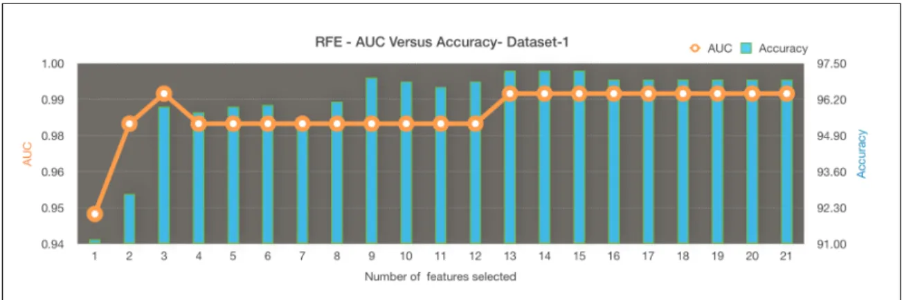
6.4.3 SVM Results with Feature Selection . . . 50

6.5 PCA Model Experiments . . . 55

6.5.1 Eigenspam projections . . . 56

6.5.2 Results . . . 56

6.6 New Dataset Creation and Experiments . . . 61

6.6.1 SVM-based Detection . . . 62

6.6.2 PCA-based Detection . . . 65

6.7 Cumulative Analysis . . . 66

7 Conclusion and Future Work . . . 69

APPENDIX A Feature Distributions . . . 75

B Feature Selection Experiments . . . 96

(10)

LIST OF TABLES

1 List of Image Features . . . 19

2 Feature Ranking Algorithm . . . 37

3 Recursive Feature Elimination Algorithm [14] . . . 38

4 KL divergence for Feature distributions . . . 46

5 Accuracy and FPR with different Kernel functions for dataset 1 . 47 6 Linear SVM Classification for dataset 1 . . . 47

7 Accuracy and FPR with different Kernel functions for dataset 2 . 49 8 RBF SVM Classification for dataset 2 . . . 49

9 Accuracy and FPR with different Kernel functions for dataset 1 using 13 features . . . 53

10 Linear SVM Classification for dataset 1 with 13 features . . . 53

11 Accuracy and FPR with different Kernel functions for dataset 2 using 12 features . . . 54

12 SVM Classification for dataset 2 with 12 features . . . 54

13 Accuracy and FPR with different Kernel functions for dataset 3 . 63 14 Cumulative Results . . . 67

(11)

LIST OF FIGURES

1 Image spam as a percentage of overall spam for the year 2015 . . 2

2 Spam Images . . . 6

3 Maximum margin of seperation . . . 12

4 Linear seperation . . . 12

5 Tranformation to higher dimension . . . 13

6 SVM weight vector . . . 15

7 Eigenvector [6] . . . 23

8 PCA Example . . . 24

9 Facial images . . . 27

10 Eigenfaces . . . 27

11 Known test image mapped to training set . . . 28

12 Unknown test image mapped to training set . . . 28

13 SVM-based detection model . . . 33

14 Feature extraction illustration of a Ham Image . . . 35

15 Feature extraction illustration of a Spam Image . . . 36

16 Eigenspam based detection model . . . 39

17 ROC curve with shaded area . . . 42

18 Feature distribution for spam versus ham images . . . 44

19 ROC curves for the feature distributions in Figure 18 . . . 45

(12)

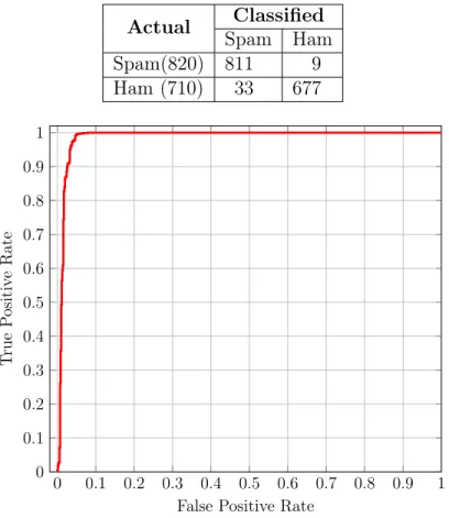
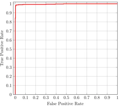
21 ROC Curve for SVM classification without feature selection for dataset 1 with AUC = 0.99 . . . 48 22 ROC Curve for SVM classification without feature selection for

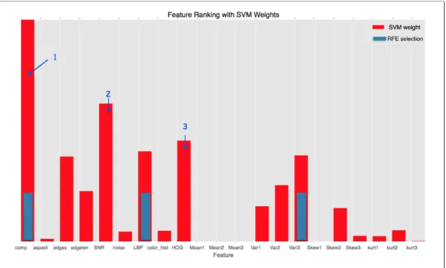
dataset 2 with AUC =1.0 . . . 49 23 RFE selection - AUC versus accuracy for dataset 1 . . . 51 24 AUC - RFE versus ranking for dataset 1 . . . 51 25 SVM weights ranking with RFE selection in blue bars for dataset 1 52 26 ROC Curve for SVM classification with RFE feature selection for

dataset 1 with AUC =0.99 . . . 53 27 RFE selection - AUC versus accuracy for dataset 2 . . . 54 28 ROC Curve for SVM classification with RFE feature selection for

dataset 2 with AUC =1.0 . . . 55 29 AUC comparison of dataset 1 and dataset 2 using feature selection 55 30 Spam Images from Training set . . . 56 31 Eigenspam - Eigenvectors corresponding to Images in Figure 30 . 57 32 Scatterplot of score for dataset 1 . . . 58 33 ROC Curve for Eigenspam with AUC = 0.99 for dataset 1 . . . . 58 34 Eigen components versus AUC for dataset 1 . . . 59 35 Scatterplot of score for dataset 2 . . . 60 36 ROC Curve for Eigenspam with AUC = 0.99 for dataset 2 . . . . 60 37 Eigen components versus AUC for dataset 2 . . . 61 38 New Spam Images . . . 62 39 Feature distribution for spam versus ham images for dataset 3 . . 63 40 AUC for the feature distributions of dataset 1 and dataset 3 . . . 64 41 ROC Curve for SVM with AUC = 0.76 for dataset 3 . . . 64

(13)

42 Scatterplot for Eigenspam Score for dataset 3 . . . 65

43 ROC Curve for Eigenspam with AUC = 0.48 for dataset 3 . . . . 66

44 ROC curves for our proposed approaches for all datasets . . . 67

A.45 Feature Distribution and ROC for Compression Ratio . . . 75

A.46 Feature Distribution and ROC for Aspect Ratio . . . 76

A.47 Feature Distribution and ROC for Edge Count . . . 77

A.48 Feature Distribution and ROC for Average Edge Length . . . 78

A.49 Feature Distribution and ROC for Signal to Noise Ratio . . . 79

A.50 Feature Distribution and ROC for Entropy of Local Binary Pattern 80 A.51 Feature Distribution and ROC for Entropy of color histogram . . 81

A.52 Feature Distribution and ROC for Entropy of HOG . . . 82

A.53 Feature Distribution and ROC for Variance of First Color Channel 83 A.54 Feature Distribution and ROC for Variance of Second Color Chan-nel . . . 84

A.55 Feature Distribution and ROC for Variance of Third Color Channel 85 A.56 Feature Distribution and ROC for Skew of First Color Channel . 86 A.57 Feature Distribution and ROC for Skew of Second Color Channel 87 A.58 Feature Distribution and ROC for Skew of Third Color Channel 88 A.59 Feature Distribution and ROC for Kurtosis of First Color Channel 89 A.60 Feature Distribution and ROC for Kurtosis of Second Color Chan-nel . . . 90

A.61 Feature Distribution and ROC for Kurtosis of Third Color Channel 91 A.62 Feature Distribution and ROC for Mean First Color Channel . . . 92

(14)

A.64 Feature Distribution and ROC for Mean of Third Color Channel . 94

A.65 Feature Distribution and ROC for Entropy of Noise . . . 95

B.66 SVM Weight Ranking . . . 96

B.67 ROC for SVM Ranking Feature Selection 1 Feature Subset . . . . 97

B.76 ROC for SVM Ranking Feature Selection 10 Feature Subset . . . 101

B.81 RFE Selection for 1 Feature Subset . . . 104

(15)

C.101 Scatterplot and ROC for Eigen Component = 1 . . . 113

(16)

(17)

CHAPTER 1 Introduction

Electronic mail, commonly known as e-mail, is the most widely used application for exchanging digital messages across the globe [17]. The usefulness of e-mail is threatened by spamming, which is defined as unsolicited bulk e-mail. Spam e-mail may, for example, contain advertisements, links to phishing websites or malware at-tached as executable files. Spam is illicit in nature, targeting numerous recipients around the world.

According to Symantec [36], during 2015 spam accounted for approximately 60 percent of all inbound e-mail, making spam filtering necessary for the continued utility of e-mail. The first generation of spam e-mail contained only text messages. As spam filters became more effective, spammers developed various techniques to bypass such filters. Image spam, which consists of spam text embedded within an image, is used by spammers as a means of evading detection. It has been reported that image spam is around 40 percent of the overall spam traffic, and this percentage continues to rise. Figure 1 shows image spam as a percentage of overall spam volume for the year 2015 as reported by Trustwave [34].

Previous approaches to detecting image spam consist of extracting various image properties and classifying the images as either spam or ham (i.e., non-spam), using machine learning techniques. This previous work either obtains low accuracy [9, 12, 39] or has an unrealistically high computational complexity [7, 19].

In this research, we develop and analyze two techniques for distinguishing spam images from ham. Specifically, we extract high-level and low-level image properties

(18)

Figure 1: Image spam as a percentage of overall spam for the year 2015

and use a feature selection algorithm based on Support Vector Machines (SVM) to minimize the computational complexity of the model. We also consider a technique based on Principal Component Analysis (PCA), and compare these two approaches. These techniques both perform very well against current spam images. We then use insights gleaned from our detection techniques to develop a more challenging class of spam images. This dataset should prove valuable for improving image spam detection capabilities.

The remainder of this paper is organized as follows. Chapter 2 provides an overview of image spam and related work on detection techniques. Chapter 3 de-scribes Support Vector Machines and the presents our selective approach based on this technique. Chapter 4 briefly explains the face-recognition technique called Eigen-faces, followed by our method of Eigenspam. Chapter 5 gives the implementation details for our techniques. Experimental results and performance analysis are pre-sented in Chapter 6. Finally, Chapter 7 provides the conclusion and possible future enhancements to the current study.

(19)

CHAPTER 2 Background

Spamming refers to sending unsolicited electronic messages to a large group of users arbitrarily. The evolution of the spam began with the idea of advertising var-ious products. Later, it had been practiced as a prank in the gaming field and also advanced to include some malicious activities. But, the focus of spamming has par-ticularly moved to e-mail, where it prevails today. Since the advertisers have no operating costs except to obtain the servers, mailing lists and the infrastructures, it has proven to be economically viable. And as there is no particular barrier, spammers have emerged numerously and are not being held for their mass mailings. In the year 2015, the predicted figure for spam messages is around seven trillion [18]. Public and several organizations had to borne the costs that include loss of productivity and bandwidth.

2.1 Types of Spam

Spam takes different forms based on the targeted media such as email spam, mobile spam, social networking spam, gaming spam [20].

Email spam is the unsolicited bulk email and the most commonly encountered spam. Identical messages are sent to numerous recipients by email; that may contain advertisements, links to phishing sites or some malware attached. Different email spam techniques include blank spam, image spam, and text spam. Initially, spam was only text based, i.e., spam email contained text in the body of the message. As the filters could classify these text messages, spammers introduced a sophisticated image-based technique. Image spam is an obfuscation method in which the text is

(20)

embedded in an image and displayed in the mail. Blank spam as the name suggests does not contain any message. It is a kind of dictionary harvest attack to collect valid email addresses.

Social spamtargets the most common social networking sites such as Facebook and Twitter. Spammers hack into the accounts and send some false links to the user’s trusted contacts.

Mobile spam aims at the text messaging service of a mobile device. “SpaSMS” is coined to describe the spam SMS [33]. Mobile spamming not only causes inconve-nience to the customers but also could cost the incoming message. Though a huge number of people use the mobile phone, there has been a considerably less amount of mobile spam because of the cost involved with sending the messages.

Gaming Spam is a form of message flooding to the players via chat rooms or public discussion areas. It is particularly common for the spammers to sell game related items for real-world money or in-game currency.

2.2 Image Spam

Image spam is a class of email spam, which has evolved as an obfuscation tech-nique to bypass the traditional text-based spam filters. The text is embedded into a graphical image which appears as the main body of the message. The method to de-tect text spam was to identify keywords from the text and block the message. Thus, more advanced form of email spam was developed by the spammers. The process to determine if an image in an email is spam or ham is as follows [16]:

∙ First, if the sender of the email is in the black list, mark it as spam. If the email is marked as spam, then determine if the message contains an image. Though

(21)

the email is identified as spam, we can not conclude that the image included is spam. Thus, a spam filter is required to classify it as spam or ham.

∙ If an email is marked as legitimate using white-list, the image contained in the message is filtered. If it is found to be spam image, the image is displayed only with users’ consent.

∙ If a new email address is encountered and it contains an image, the image has to be filtered. If the image is detected to be spam, the image is not displayed. A choice is given to the user to mark it as spam.

2.2.1 Types of Image Spam

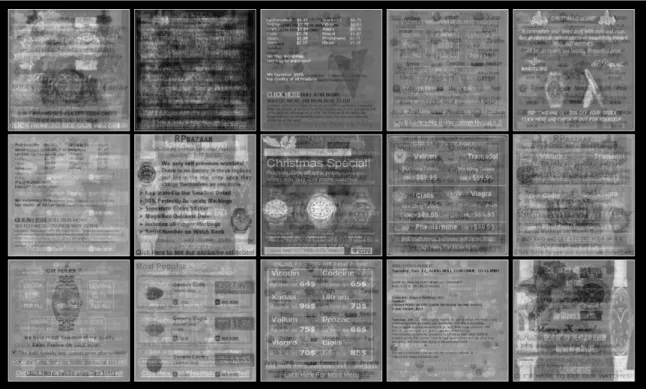
Image spam is heavy in content and has progressed in different forms to con-stantly challenge the conventional filters: Pure text image, Randomized image, Mixed image.

Pure text image is the first generation spam image and rich in text. It con-tains a pure text file embedded as a picture in the message as shown in Figure 2a. Since most e-mail clients rendered graphical images automatically, it could deliver the intended message successfully. A filtering technique that uses Optical character recognition (OCR) has been employed to identify such spam. Words from the image are extracted using OCR, and the text is passed to the traditional text-based filter.

Randomized image is introduced to increase the difficulty of filtering spam using OCR. Spammers created images by adding noise, a thin background of random artifacts, or by rotating the image slightly. These changes do not influence the read-ability of the users but significantly affect the output of the OCR based filter. The spammers also carried out some unnoticeable changes such as shading the border,

(22)

adding tiny streaks with almost random patterns to bypass the filters that are based on Hash signatures. An example of this kind is shown in Figure 2d.

A Mixed image is a form of spam that is split into multiple parts to contain both text and some related picture or an animation. These forms appear to be very close to genuine and are challenging to be detected by most of the filters. Images shown in Figure 2b and Figure 2c.

(a) (b) (c) (d)

Figure 2: Spam Images

2.2.2 Content Categories

Image spam can contain the following categories [20]:

∙ Advertisements — The content includes some details to promote a product or some online shopping offers for various

∙ Pornography — The image contains obscene pictures or products.

∙ Phishing links — Images contain a link to websites that would attempt to acquire their usernames and passwords or can also contain a link to malicious websites.

(23)

substantial amount of currency for a small payment. This fee helps the fraudster to collect a huge amount and later disappear or creates a series of the victims.

2.3 Image Spam Detection

Image spam detection techniques fall into two categories: Content-based and Noncontent-based.

2.3.1 Content-based Filter

Content-based filters inspect the image content for specific keywords typically used in the spam text. And then may use pattern recognition technique to track particular behavior or pattern. One of the early content based filters is Spam As-sasin [32], which uses OCR to extract text from the images and analyze the text using traditional text-based filters.

2.3.2 Noncontent-based Filter

The noncontent-based filter uses different properties of the image to classify the spam image. The earlier work included extracting simple metadata features and color properties of an image. This kind of filter relies on the fact that the genuine image possesses distinct characteristics compared to a computer generated image with text.

2.4 Related Work

Image spam detection has stirred interests of many researchers since the time of its birth. Various detection techniques and algorithms have been explored for an efficient classification. In this section, we present some works in the scientific literature that dealt with the image spam detection.

(24)

One of the classical techniques for the content-based filters was Spam Assasin [32], which uses Optical Character Recognition (OCR) to recover the text from the spam images. OCR is a mechanism for electronic conversion of images with any text (hand-written or printed) into machine-encoded text. The text-based filters are used for the further analysis of the extracted text. To bypass these filters, spammer used various obfuscation techniques like making the text blur which practically effected the quality of the existing filters.

The limitations of the OCR-based detection have been defeated by non-content based email spam filtering. One of the early works in this area is Learning fast clas-sifiers for image spam [7]. Authors in this paper propose a fast and robust detection method by extracting a set of features based on simple file properties and metadata. They employed Maximum Entropy, a discriminative model to evaluate the feature set. They included two other classifiers such as Naive Bayes and ID3 decision trees for com-parison and also to represent a different learning approach. The results showed that Maximum Entropy outperformed Naive Bayes while decision tree is a close second. This research also offers Just-in-Time (JIT) extraction which focuses on extracting features based on each image. The basis of the feature selection is a greedy inclusion by mutual information technique. A JIT decision tree is constructed to evaluate the feature sets. The overall system demonstrated an efficient classification.

Image spam hunter [12] proposed a detection method based on probabilistic boosting tree considering global image features like color and gradient histogram. They suggested a learning-based prototype system to differentiate spam from normal images. The system works by first clustering the spam into groups based on a similar-ity measurement of color and gradient oriented histograms. Then build a probabilistic boosting tree on the training set (chosen from the clustered groups) to distinguish

(25)

the images. Results obtained from SVM classifier are considered as a baseline for the comparison of their system. The proposed technique achieved an accuracy rate of 89.44% with 0.86% false positive rate.

A comprehensive server to client side approach for image spam detection [9] applied the clustering technique at the server end to segregate genuine and spam. Further, feature-based active learning methods have been used for classification at the client side. The server-side approach involves a sparse nonnegative representation of a similarity measure. This similarity measure is combined with a spectral clustering algorithm for analysis of spam images. SVM active classification technique is applied at the client-side to filter the spam images that have survived during the server-side detection. This system extracted a large feature set and thus increased the computational complexity though have ensured an accuracy rate of 99%.

Detecting image spam based on file properties, Hough transform, and his-togram [39] focussed the detection constrained by specific image attributes. The authors of this paper extracted features related to three different domains and com-pared their individual performance. The first approach considers features related to file properties like file format, width, height, and aspect ratio that are derived at a low computational cost. The second method uses classification based on color histograms of the image. The final approach uses Hough transforms for the classification. Hough transform is a method to find different shapes present in the images using edge de-tection. According to their experimental results, an approach using file properties eliminates around 80% of image spam and the method using the histogram to imple-ment distance measure reduces 84% of the spam images whereas the Hough transform method achieves 88% of accuracy and also minimizes the false positive rate

(26)

introduced a server side solution to extract multiple domain features and further classify based on fuzzy inference system. F-ISDS employs dimensionality reduction based on Principal Component Analysis (PCA) to reduce the number of features by mapping them to their principal components. Further, Linear Regression Analysis is used to model the relationship between the principal components and the extracted features. Based on the model, membership functions are designed for a Fuzzy Infer-ence System classifier. Though this work focused on an extensive range of features, obtained an accuracy rate of 85%.

This comprehensive study of the existing research motivated us to develop an efficient system for the image spam detection using various machine learning algo-rithms.

(27)

CHAPTER 3 SVM-based Detection

A large number of classification algorithms have been applied to spam detection area earlier. Among them, Support Vector Machine (SVM) [15] is a useful technique and famous for its good generalization performance. Previously, SVM has been widely used for text-based spam detection. As SVM provides a useful analysis by separating the hyperplane, in this work, we employed SVM for classification. In the next sections, we present an overview of SVM technique followed by our approach for image spam detection based on SVM.

3.1 SVM Overview

Support vector machines is a class of algorithms based on optimization and is used for binary classification. SVM is a supervised learning technique, which means that it requires labeled training data. That is, we must use data that has been categorized and labeled in advance. The algorithm uses the labeled data to train a model and find an optimal hyperplane that separates the two classes of the data by acting as a threshold. This technique is based on the following intuitive ideas [35]:

∙ Maximize the margin: Consider a labeled training data, we attempt to find a hyperplane that separates the data. Since it is binary classification, we try to divide the two classes with a maximum margin of separation.The margin is determined by the minimum distance between the hyperplane and any point in the training set. For example, the hyperplane is denoted by the yellow line in Figure 3. The black arrows indicate the nearest elements called the support

(28)

vectors.

Figure 3: Maximum margin of seperation

∙ Work in higher dimension: For a given data, if a hyperplane exists, we recognize the problem as linearly separable. To deal with the cases where data is not linearly separable, SVM employs a technique to move the input space to a higher plane giving additional space to find the hyperplane. For example, the data on the left side of the Figure 4 cannot obtain a linear separation. Though a parabola is possible, we can also use a transformation technique (𝜑) to map input space to feature space and determine the hyperplane.

(29)

∙ Kernel trick: This is essentially a mapping function that transforms the data into higher dimensions. Kernel trick makes it easy to compute a hyperplane in the feature space. Figure 5 shows an example where the input space on the left is not linearly separable, but after applying the transformation based on kernel trick, we can easily construct a hyperplane.

Figure 5: Tranformation to higher dimension

3.1.1 SVM Algorithm

SVM algorithm functions in two phases: Training Phase and Testing Phase. In the Training Phase, we create a model by training on a labeled dataset. In the Testing Phase, we apply the generated model to the test dataset. The test phase determines the accuracy of the given classifier. The SVM training and testing algorithms can be generalized as follows [35].

3.1.1.1 Training Phase

The SVM training phase determines the equation of a separating hyperplane that maximizes the margin. The obtained hyperplane will separate the feature space into two sets. As a result, we can classify any points during the testing phase. The

(30)

generic process involves solving Lagrangian Duality [35]. The simplified steps of SVM Training Phase algorithm is given below.

1. Consider a set of labeled training data consisting of points 𝑋1, 𝑋2, . . . , 𝑋𝑛 and

a corresponding set of classification𝑧1, 𝑧2, . . . , 𝑧𝑛, where𝑧𝑖 ∈ {−1,1}.

2. Select a kernel function 𝐾 and a parameter 𝐶, which specifies the permissible number of classification errors.

3. Solve the optimization problem Maximize: 𝐿(𝜆) = 𝑛 ∑︁ 𝑖=1 𝜆𝑖− 1 2 𝑛 ∑︁ 𝑖=1 𝑛 ∑︁ 𝑗=1 𝜆𝑖𝜆𝑗𝑧𝑖𝑧𝑗𝐾(𝑋𝑖, 𝑋𝑗) Subject to: 𝑛 ∑︁ 𝑖=1 𝜆𝑖𝑧𝑖 = 0 and 𝐶 ≥𝜆𝑖 ≥0 for 𝑖= 1,2, . . . , 𝑛 (1) to obtain 𝜆𝑖 and 𝑏. 3.1.1.2 Testing Phase

Given a trained SVM, we score a data point by determining on which side of the separating hyperplane it resides. The process involves the following steps.

1. Given a datapoint X, we compute score 𝑓(𝑥) =

𝑠

∑︁

𝑖=1

𝜆𝑖𝑧𝑖𝐾(𝑋𝑖, 𝑋) +𝑏 (2)

where𝑠 is the number of support vectors and is much smaller than𝑛. This can also be written as

𝑓(𝑥) =𝑤·𝑥+𝑏 where 𝑤=𝜆𝑖𝑧𝑖𝐾(𝑋𝑖, 𝑋). (3)

This 𝑤is called the weight vector which represents the support vectors orthog-onal to the hyperplane in the Figure 6.

(31)

Figure 6: SVM weight vector 2. Classify X according to 𝑐(𝑋) = ⎧ ⎪ ⎪ ⎨ ⎪ ⎪ ⎩ 1 if 𝑓(𝑋)>0 −1 otherwise. (4) 3.1.2 Kernel Functions

A Kernel function 𝐾, accepts inputs as𝑋𝑖 and𝑋𝑗 and produces an output that

is the inner product of their respective images, 𝜑(𝑋𝑖) and 𝜑(𝑋𝑗) [5]. The function is

given by

𝐾(𝑋𝑖, 𝑋𝑗) =𝜑(𝑋𝑖)·𝜑(𝑋𝑗)

which represents a dot product of the input data points mapped onto the higher dimensional feature space by 𝜑 transformation. There are different Kernel functions used in practice. SVM classifier allows the user to specify one of the following kernels:

∙ Linear Kernel:

(32)

∙ Polynomial Kernel:

𝐾(𝑋𝑖, 𝑋𝑗) = (𝑋𝑖·𝑋𝑗 + 1)𝑝

∙ Radial basis function:

𝐾(𝑋𝑖, 𝑋𝑗) =𝑒−(𝑋𝑖−𝑋𝑗)(𝑋𝑖−𝑋𝑗)/(2𝜎

2₎

∙ Two Layer perceptron:

𝐾(𝑋𝑖, 𝑋𝑗) = tanh(𝛽0(𝑋𝑖 ·𝑋𝑗) +𝛽1)

Choosing the correct kernel is a nontrivial task. The classification generally depends on tuning the kernel parameters no matter which kernel is chosen.

3.2 Selective Approach using SVM

In this paper, we present a novel approach based on the SVM algorithm that allows a sensitive feature selection apart from the traditional feature extraction. Then, creates a model for fast and accurate classification. The baseline of the system is the fact that the characteristics of a spam image, which is computer generated are distinct from a genuine camera generated image [7]. Our empirical evaluation shows that our model yields high accuracy with a reduced computational cost. With this approach, we extract a broad set of features from various domains. A feature selection algorithm based on SVM weights has been used to select a subset containing highly distinguishing features to make the classification easy. Thus, our model employs Feature Extraction, Feature Selection, and Classification, which we discuss further in detail.

(33)

3.2.1 Feature Extraction

In this feature extraction module, we detect and isolate various desired portions or shapes of a digitized image as a compact feature descriptor or feature vector [26]. We extract an effective set of 21 discriminant image features. These features have been identified from various image property domains that classify a computer-generated image and a camera-generated image. Various features have been employed in the previous related work for noncontent-based filtering. After rigorous simulation and empirical analysis, we chose the following image statistics from the literature to inte-grate color, shape, metadata, noise and appearance properties.

∙ Color Domain: Considering that the spam images are composed of fewer color shades compared to the genuine images, we extract color related properties to classify the images. We compute the entropy of the color histogram as the first image feature. By quantizing each color band in the RGB space, the color histogram depicts the distribution of colors in an image. We further set up a histogram for the three color channels separately and then compute the mean, variance, skewness and kurtosis for each, which adds another 12 feature statistics [9].

∙ Texture Domain: Local binary pattern (LBP) [22] labels the pixel of an image by thresholding the neighborhood pixels. This shows the similarity or differences between the neighboring pixels. The entropy of the LBP histogram is calculated as one texture feature [9]. The natural images are likely to have more information in this feature vector as they are captured with a wide variety of backgrounds and foregrounds.

(34)

the local object appearance and shape within an image. It can be described by the distribution of the intensity gradients; that is the directional change in the intensity of the image. The entropy of the gradient magnitude orientation histogram is the first shape feature [11]. Then we use edges of the image to compute the next two image features. The curved line segments formed by a set of points where image brightness change sharply are called edges [3]. The total number of edges and the average length of the edges are examined for our classification [10]. As spam images are generally a combination of text and images, they are supposed to have more number of edges compared to the ham images.

∙ Metadata Domain: Compression ratio and Aspect ratio of the images are calculated as the two metadata features [39]. Compression ratio captures the amount of compression achieved by calculating the ratio of pixels in an image to an actual image size. Aspect ratio is a proportional ratio between width and height of an image. Spammers try to compress the picture to minimize the size of the email which discriminates from a genuine one.

∙ Noise Domain: Image noise is the random change of brightness or color in-formation in images and is an aspect of electronic noise. The effects of the noise content are analyzed by computing entropy of noise and signal to noise ratio which is the measure of sensitivity [19]. Genuine images are captured in varied backgrounds tend to have more noise than spam images unless noise is artificially added.

Table 1 gives the list of all the features with the abbreviations as used in the rest of the paper.

(35)

Table 1: List of Image Features

Feature No. Feature Name Abbreviation used

f1 Entropy of Local Binary Pattern Histogram LBP

f2 Entropy of Histogram of Oriented Gradients HOG

f3 Number of Edges Edge no

f4 Average length of Edges Edge len

f5 Compression Ratio Comp

f6 Aspect Ratio Aspect

f7 Signal to Noise Ratio SNR

f8 Entropy of Noise Noise

f9 Entropy of Color Histogram Color hist

f10 Mean of Red Channel Mean1

f11 Mean of Blue Channel Mean2

f12 Mean of Green Channel Mean3

f13 Variance of Red Channel Var1

f14 Variance of Blue Channel Var2

f15 Variance of Green Channel Var3

f16 Skewness of Red Channel Skew1

f17 Skewness of Blue Channel Skew2

f18 Skewness of Green Channel Skew3

f19 Kurtosis of Red Channel Kurt1

f20 Kurtosis of Blue Channel Kurt2

f21 Kurtosis of Green Channel Kurt3

3.2.2 Feature Selection

In the feature selection module, we select a subset of highly discriminant features for our model construction [2]. The aim is to mute out features that are not useful to the existing features during classification. The feature selection could invariably reduce the computational complexity and increase the speed. There are various al-gorithms for ranking the features. In this paper, we explored a different perspective of Support Vector Machines(SVM) for feature ranking. Feature selection using SVM was earlier used for identification of gene subsets in biological research [14]. In this section, we describe two feature selection strategies that we analyzed.

(36)

3.2.2.1 Feature Ranking using SVM Weights

Recall that in linear SVM,𝑤is the weight vector that represents the coordinates of the support vectors orthogonal to the resultant hyperplane in equation (3). The dot product of this weight vector with any point from the test set gives the direction of the predicted class. So using the weight vector we find the most useful feature for separating the data with the fact that the hyperplane would be orthogonal to that axis. The absolute size of this weight coefficient relative to the other points gives an indication of how useful the feature is during the classification [24]. Our first approach for feature selection is based on the weights as ranking criteria to limit the number of features. Weight vectors are evaluated by training the model using linear SVM. Then𝑛 features with the largest absolute value of the weight are marked as the most important features. This is intended to reduce the computational effort during the test phase. The steps for this algorithm to select a subset of𝑛 features are as follows:

1. Train the classifier using Linear SVM using the feature set 2. Compute the SVM weights for all the features

3. Select the first 𝑛 features with the largest weights 4. Create a model based on the subset

3.2.2.2 Recursive Feature Elimination using SVM Weights

The usual feature ranking criteria becomes very sub-optimal when it comes to removing several features at a time, which is necessary to obtain a small and accu-rate feature subset. This problem is overcome by using an iterative procedure called Recursive Feature Elimination (RFE) [14]. RFE is designed to recursively remove the attributes and build a model on the remaining attributes. It relies on the model

(37)

accuracy to identify the combination of attributes that contribute the most to pre-dicting the target attribute. Here we used linear SVM as the model. The steps for the RFE algorithm are as follows:

1. Train the classifier using Linear SVM using the feature set 2. Compute the ranking criterion using SVM weights

3. Remove the feature with smallest ranking criterion

4. Repeat steps 1 to 4 until number of features in the subset matches the criteria

3.2.3 Classification

The model generated after feature selection is applied to the test set. Selected features are extracted from the test set images. Then the SVM technique is used for classifying the two classes of spam and ham images. Different kernel functions have been applied during the empirical testing, and the analysis is presented in Chapter 6.

3.3 New Spam Data

In previous section, we discussed the SVM weight vectors which reveal the im-portance of the features by training a model. The weight vectors not only help to minimize the computational effort but also expose the determinant characteristics of the spam images. This fact motivated us to create a new set of spam images that would attempt to conceal all the visible traits of the original spam images. This has been explained in detail in Chapter 6.

(38)

CHAPTER 4 PCA-based Detection

In this chapter, we focus on PCA-based image spam detection strategy. In com-parison to the earlier detection technique, this approach also depends on the struc-tural entropy score but does not involve feature extraction for the images. Principal Component Analysis (PCA) is a linear transformation method that finds the direc-tions (principal components) of the data and maximizes the variance. PCA relies on eigenvector analysis which is also achieved using Singular Value Decomposition (SVD) [35].

First, we briefly discuss the mathematical model of eigenvalues and eigenvectors that helps us for the theoretical discussion of PCA in the following section. Then we review Eigenfaces, an application of PCA to the well-known facial recognition problem from [37], which forms the basis for our “Eigenspam” detection technique. We present the implementation and experimental analysis in the coming chapters.

4.1 Eigenvalues and Eigenvectors

Eigenvalues and eigenvectors are prominently used in the interpretation of linear transformations. The term eigen means “unique to”, or “peculiar to” in the sense of “characteristic” [41]. It was initially designed to analyze principal axes of the rotational motion of rigid bodies.

In linear algebra, eigenvector is a non-zero vector 𝑥 for a square matrix 𝐴 that satisfies 𝐴 = 𝜆𝑥 where 𝜆 is scalar called eigenvalue. Eigenvector 𝑥 of a matrix 𝐴 implies that 𝐴 stretches the eigenvector𝑥by𝜆, without changing the direction.

(39)

Fig-ure 7 depicts a vector 𝑥 and its geometrical transformation 𝜆𝑥. It shows that for a particular matrix 𝐴 and a vector 𝑥, the effect of 𝐴𝑥 is same as scalar multiplication of eigenvector 𝑥with a magnitude given by its eigenvalue 𝜆. Considering each eigen-value is associated with an eigenvector, the relative importance of an eigenvector is given by the magnitude of its corresponding eigenvalue and hence can be used for dimensionality reduction of data by removing the unimportant directions.

Figure 7: Eigenvector [6]

4.2 Principal Component Analysis

PCA is a linear algebra technique which helps us find the most significant direc-tions in the data that enables to reduce the dimensionality of the problem. In simple terms, PCA is a way to identify patterns in the data and express them to identify the similarities and differences. If the data is of higher dimension, it is hard to find the patterns without any graphical representation. PCA minimizes this problem by reducing the dimensionality. The main idea of PCA for a given dataset 𝑆 with 𝑛 variables is to define this dataset with a smaller set of elements that are linear com-binations of the original values. These elements are called the principal components. For example, consider the a scatterplot of the scores from an experiment as shown in Figure 8a. The minimal spanning set of the data is not very informative, so we

(40)

try to reduce the dimensionality. We can use a regression line as shown in Figure 8b, which is the best-fitting straight line to the set of points. This regression line reduces the dimensionality by obtaining the significant information but there is also some loss of information. PCA also uses linear regression but provides a better basis that reveals the structure for viewing the data. Figure 8c illustrates this basis, where the direction determines the structure and the length measure gives the variance of the data in the given direction. PCA thereby eliminates the less informative directions proportional to the variance to reduce the dimensionality.

(a) Experiment Data (b) Regression Line (c) PCA Basis Figure 8: PCA Example

The process of dimensionality reduction using PCA consists of following steps [31].

1. Consider an experimental data as matrix 𝐴𝑚×𝑛, where 𝑛 is the number of

ex-periments, and 𝑚 is the number of measurements per experiment.

2. Compute the mean of each row and subtract it from the each element of the corresponding row.

3. Construct a covariance matrix 𝐶 = _𝑛1𝐴𝐴𝑇_{. Each element on the principal}

(41)

the off-diagonal element is the covariance. We use the covariance matrix [40] to determine the principal components.

4. To diagonalize the covariance matrix, compute the eigenvalues and eigenvectors of the matrix 𝐶.

The diagonalized matrix reveals the inherent structure of the data. Also, the dominant eigenvalues correspond to the most informative directions of the data. Thus, we use this information to reduce the dimensionality of the problem. In the next section, we discuss a classical application of PCA for facial recognition.

4.3 Eigenfaces

Eigenfaces [37] is a technique that is widely used for face recognition and is based on PCA. Eigenfaces approach interprets the complex problem of face recognition as a 2-dimensional problem by assuming faces to be upright and ignoring the geometric features of the face, which makes it computationally simple.

4.3.1 Face Recognition

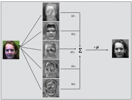
For this approach, first, a set of training images is considered with the faces of images centered. A covariance matrix is constructed with the pixel values from the images. Eigenvectors of this covariance matrix are computed to measure the similarity between different images. These vectors are referred to as “eigenfaces”. The eigenfaces exhibit significant features of a face but do not certainly present intuitive features such as lips, eyes, etc. The feature space defined by these eigenfaces is termed as “face space”.

(42)

vector for each image in the training set is obtained. These set of weights are used to score any image. Consider an unknown image is given for classification, the image is first projected onto the face space. The Euclidean distance to each of the training images from the weight vector of the projected image is computed. The minimum of these distances defines the score. If the score is small, then the image is considered to be the closest match to a class in the training set, else the image does not belong to that class.

To illustrate this process, consider the images in Figure 9 to be the training set. The training images have been downloaded from Yale face database [42] for experiments. Then the corresponding eigenfaces as in Figure 10 are obtained by projecting the training images onto the face space with most significant eigenvalues. An image from the training set can be reconstructed using its eigenvectors. That is, if a projected image belongs to the training set, it could be matched by reconstructing its eigenfaces as shown in Figure 11. When a unknown image is projected onto the face space, the results may be entirely different as shown in Figure 12. That is, even though a test image is not in the training data, an image with lowest score is recognized and mapped. To overcome this anomaly, we use a certain threshold to actually classify the images.

4.4 Eigenspam

The face recognition technique using eigenvectors [37] inspires our approach to detect spam images. As images of different people have similarities corresponding to the outline of their facial features, different spam images also have some common characteristics like the wild backgrounds and the text. For the following section, we will refer to “Eigenspam” as the set of eigenvectors that constructs a spam image as

(43)

Figure 9: Facial images

Figure 10: Eigenfaces

corresponds to Eigenfaces, which constructs the face when combined linearly. The training phase and testing phase for the system are discussed in detail below [35].

(44)

Figure 11: Known test image mapped to training set

Figure 12: Unknown test image mapped to training set

4.4.1 Training Phase

The Training phase is the stage during which our model is trained by a database of different spam images called the training set. We determine the eigenvectors and

(45)

project them onto the eigenspace to compute the weight vectors. The training phase consists of the following steps:

1. Acquire a set of 𝑀 spam images, resize all images to be of same dimensions. 2. Convert each image to greyscale. Each image is represented as a vector 𝑉𝑖 by

converting to greyscale and flattening the image. Since all images are resized to same dimensions, each image consists of a same number of pixels. We represent the entire image set as 𝑁 ×𝑀, where 𝑁 is the count of pixels in each image, and 𝑀 is the number of images.

3. Compute the mean image vector and subtract from each image. Let 𝑒𝑖(𝑉) be

the 𝑖𝑡ℎ _{element of the vector}_𝑉_{. Then, for} _𝑗 _{= 1}_,₂_,₃_{, . . . , 𝑁,} _{we let}

𝜇𝑗 =

1

𝑀 ∑︁

𝑖𝑒𝑗(𝑉𝑖),

that is, 𝜇𝑗 is the mean of the elements appearing in position 𝑗 of the training

vectors𝑉𝑖. The vector of means is defined as

𝜇= ⎛ ⎜ ⎜ ⎜ ⎝ 𝜇1 𝜇2 .. . 𝜇𝑁 ⎞ ⎟ ⎟ ⎟ ⎠

Subtract the mean from each vector 𝑉.

˜

𝑉𝑖 =𝑉𝑖−𝜇

The matrix of interest is defined as

𝐴= ( ˜𝑉1 𝑉˜2 . . . 𝑉˜𝑀) (5)

that is, column𝑖of𝐴is the vector𝑉˜𝑖. By construction, the mean of the elements

(46)

4. The covariance matrix [23] is

𝐶 = 1

𝑀𝐴𝐴

𝑇

and the elements of the matrix𝐶 are denoted as 𝑐𝑖𝑗. Then

𝑐𝑖𝑗 =

˜

𝑉𝑖·𝑉˜𝑗

𝑀 (6)

where 𝑉˜𝑖·𝑉˜𝑗 denotes the dot product.

5. Find the normalized eigenvectors of covariance matrix𝐶. However,𝐶is𝑁×𝑁, where𝑁 is the number of pixels of an image in the training and the number𝑁 is generally large. So, instead of instead of directly computing the eigenvectors of 𝐶, we use the following efficient approach.

Suppose a matrix𝐿

𝐿=𝐴𝑇𝐴 (7)

Here𝐿is a 𝑀×𝑀 matrix. Since𝑀 is the number of the images in the training set, it will be much smaller than 𝑁. Let 𝜈 is an eigenvector of 𝐿, that is,

𝐿𝜈 =𝜆𝜈 for some 𝜆. Then multiplying by𝐴

𝐴𝐿𝜈 =𝐴𝐴𝑇𝐴𝜈 =𝐴𝜆𝐴𝜈

and thus, 𝐴𝜈 is the eigenvector of 𝐶 with a corresponding eigenvalue 𝜆.

6. Suppose that the set of eigenvectors of 𝐿 from the above step is 𝜈 = {𝜈1, 𝜈2, . . . , 𝜈𝑗} and obtain the corresponding eigenvectors of𝐶 using 𝜇𝑖 =𝐴𝜈𝑖,

for 𝑖= 1,2, . . . , 𝑗. Thus, consider the eigenvectors of𝐶 as 𝑢= (𝑢1, 𝑢2, . . . , 𝑢𝑀)

(47)

7. Since we have already mentioned that the most significant eigenvectors corre-spond to the eigenvalues with the largest magnitude. We select the first 𝑚 singular vectors of 𝑢𝑖 where 𝑚 ≤ 𝑀 and ignore eigenvectors with small

eigen-values.

8. Project each image of the training set 𝑉 onto the eigenspace [41]. We compute weight vectors Ω𝑖, for𝑖= 1,2, . . . , 𝑀, as

Ω𝑖 = ⎛ ⎜ ⎜ ⎜ ⎝ ˜ 𝑉𝑖·𝑢1 ˜ 𝑉𝑖·𝑢2 .. . ˜ 𝑉𝑖·𝑢𝑚 ⎞ ⎟ ⎟ ⎟ ⎠ (8)

where the dot product for the vectors 𝑥 = (𝑥1, 𝑥2, . . . , 𝑥𝑛) and 𝑦 =

(𝑦1, 𝑦2, . . . , 𝑥𝑛)is defined as 𝑥·𝑦= 𝑛 ∑︁ 𝑗=1 𝑥𝑗𝑦𝑗.

9. Finally, define the scoring matrix ∆

∆ = (Ω1,Ω2, . . . ,Ω𝑚). (9)

Thus, we can view ∆as a model that is trained using images in 𝑉.

4.4.2 Testing Phase

In the testing phase, a new image is projected onto the eigenspace of the training set and the Euclidean distance is computed between the test image weight vector and each of the weight vectors of the training set images. If the distance measure, also called as the score, is below a certain threshold, then the test image is classified as a spam image or it is marked as a ham image. Given an image vector 𝑋 that we want to score, we proceed as follows.

(48)

1. Analogous to (8), we compute the weight vector, 𝑊 of 𝑋˜ where 𝑋˜ =𝑋−𝜇, 𝑊 = ⎛ ⎜ ⎜ ⎜ ⎝ 𝑤1 𝑤2 .. . 𝑤𝑚 ⎞ ⎟ ⎟ ⎟ ⎠ = ⎛ ⎜ ⎜ ⎜ ⎝ ˜ 𝑋𝑖·𝑢1 ˜ 𝑋𝑖·𝑢2 .. . ˜ 𝑋𝑖·𝑢𝑚 ⎞ ⎟ ⎟ ⎟ ⎠ (10)

2. Compute each Euclidean distance between 𝑊 from (10) and weight vector Ω𝑖

in (9). Suppose𝜖𝑖 is the distance between 𝑊 and Ω𝑖, then

𝜖𝑖 =𝑑(Ω𝑖, 𝑊).

3. Finally, determine the score

score(𝑋) = min

𝑖 (𝜖𝑖).

This score(𝑋) determines how closely the input image represents the spam image features among the training set. The smaller the score, the better is the match to the training set image. The classification of the images is based on a threshold value for the score and is set experimentally.

(49)

CHAPTER 5 Implementation

This chapters discusses the implementation of the techniques presented in the previous chapters. The first section gives implementation details of the SVM-based approach and the second section gives the implementation of PCA-based detection.

5.1 SVM-based Detection

We have implemented SVM using Python’s Scikit-Learn package [30]. The sup-port vector machines in Scikit-Learn supsup-ports both dense and sparse vectors as input. Internally it uses libsvm [4] library to handle all the computations. It also provides an option to train the classifier with different kernel functions. Figure 13 shows the internal working of our SVM-based approach for image spam detection. We discuss the training phase and testing phase executions in detail in the following sections.

(50)

Initially, we construct a training set with a combination of spam and ham images. The feature extraction module takes images as input and generates a CSV file with a list of images and the corresponding feature values. The feature selection module takes this CSV file as input to create a model and return the subset of features selected.

5.1.1.1 Feature Extraction Module

We represent the train set images as 𝑀 ×𝑁 matrix, where 𝑀 is the number of images and 𝑁 is pixel count . We extract a broad set of features for each of the train set images by manipulating the array. To obtain the entropy of color histogram, we first build a103 _{dimension color histogram in the joint RGB space by quantizing each}

color band [7]. The entropy of the color histogram is then computed. We further set up one 100-dimensional histogram for each of the three color channels. Then mean, variance, skewness and kurtosis for each of the three histograms are calculated. The entropy of the LBP histogram is calculated as one texture feature. We extract 59 -dimensional texture histogram, including 58 bins for all the different uniforms local binary pattern and measure the entropy value. A 40×8 = 320-dimensional gradient magnitude-orientation histogram is built to describe the shape information. The entropy of the gradient magnitude orientation histogram is the first shape feature. The total number of edges and the average length of the edges are computed by running Canny edge detector [3]. Compression ratio is computed using following:

Compression ratio= height×width×bit depth

file size

Aspect ratio is measured as the ratio between the width and height of the image. Signal to noise ratio is computed as the proportional relationship between mean and

(51)

variance. The noise of the image is measured by measuring deviation at each pixel of the image.

To illustrate the feature extraction, consider a picture as shown in Figure 14a. The color histogram of three different channels (RGB) are computed and plotted as shown in Figure 14b. The image is then converted to a greyscale as presented in Figure 14c. We use Canny edge detector to detect the edges. With a variation in the parameters, the edges could be detected as shown in Figure 14d and 14d. The histogram of oriented gradients (HOG) is computed and displayed as in Figure 14f. The similar illustration is also presented for a spam image in Figure 15. Finally, the entropy of these histograms is computed as feature vectors.

(a) Ham Image (b) Color Histogram _{(c) Greyscale}

(d) Canny edges𝜎 = 1 (e) Canny edges 𝜎= 3 (f) HOG Figure 14: Feature extraction illustration of a Ham Image

(52)

(a) Spam Image (b) Color Histogram (c) Greyscale

(d) Canny edges𝜎 = 1 _{(e) Canny edges} _𝜎_{= 3} (f) HOG Figure 15: Feature extraction illustration of a Spam Image

5.1.1.2 Feature Selection Module

The extracted features along with the class label (1 for spam and −1 for ham) are given as input to a linear SVM classifier. We generate a model after selecting a subset of features using SVM weights. Feature ranking using linear SVM weights has been implemented using the algorithm described in Table 2.

Recursive feature elimination algorithm has been implemented based on the al-gorithm [14] in Table 3. A model is generated using the selected features. This model is used to classify the images.

(53)

Table 2: Feature Ranking Algorithm

// Input: Training set 𝑋0 = [𝑥1, 𝑥2, . . . , 𝑥𝑘, . . . , 𝑥𝑛]𝑇,

// Class labels 𝑦= [𝑦1, 𝑦2, . . . , 𝑦𝑘,. . .¸ , 𝑦𝑛]𝑇

// Output: Feature ranked list 𝑟 // Initializations

Set of features 𝑆 = [1,2, . . . , 𝑚], Feature ranked list 𝑟= [ ]

Max count of features to be selected =𝑠 Begin

Train the classifier

𝜆=SVM-Train(𝑋, 𝑦)

Compute the weight vector of dimension length(𝑆)

𝑤=∑︀

𝑘

𝜆𝑘𝑦𝑘𝑥𝑘

Compute the ranking criteria 𝑐𝑖 = (𝑤𝑖)2,for all 𝑖

Sort the features based on weights 𝑓 =sort(𝑐)

Update feature ranked list 𝑟= [𝑆(𝑓), 𝑟]

Select the first 𝑠 features 𝑆 =𝑆(𝑠)

Return 𝑟, 𝑆 End

5.1.2 Testing Phase

A test set of spam and ham images is given as input to the feature extraction module to extract the selected subset of features. Then the extracted features are classified using SVM algorithm.

(54)

Table 3: Recursive Feature Elimination Algorithm [14]

// Input: Training set 𝑋0 = [𝑥1, 𝑥2, . . . , 𝑥𝑘, . . . , 𝑥𝑛]𝑇,

// Class labels 𝑦= [𝑦1, 𝑦2, . . . , 𝑦𝑘, . . . , 𝑦𝑛]𝑇

// Output: Feature ranked list 𝑟 // Initializations

Subset of surviving features 𝑆 = [1,2, . . . , 𝑚], Feature ranked list 𝑟= [ ]

Begin

Repeat until 𝑆 = [ ]

Constrain training𝑋to feature set𝑆 𝑋 =𝑋0(:, 𝑆)

Train the classifier

𝜆=SVM-Train(𝑋, 𝑦)

Compute the weight vector of dimension length(𝑆)

𝑤=∑︀

𝑘

𝜆𝑘𝑦𝑘𝑥𝑘

Compute the ranking criteria 𝑐𝑖 = (𝑤𝑖)2,for all 𝑖

Find feature with smallest ranking criterion 𝑓 =argmin(𝑐)

Update feature ranked list 𝑟= [𝑆(𝑓), 𝑟]

Discard feature with smallest rank 𝑆 =𝑆(1 : 𝑓−1, 𝑓 + 1 :length(𝑆))

Return 𝑟 End

5.2 PCA-based Detection

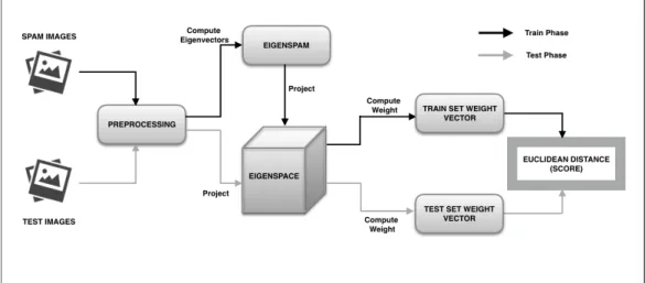
We implemented the algorithm discussed in Chapter 4 using Python. Python Imaging Library (PIL) and OpenCV packages have been used to work with the images. Figure 16 summarizes the eigenspam detection process.

(55)

Figure 16: Eigenspam based detection model

We construct a test set of spam images. Initially, we resize all the images and convert them to grayscale. Converting to grayscale, flattens the image and allows us to store in a matrix𝐴𝑀×𝑁, where𝑁 is total pixel count of an image and𝑀 is a total

number of image files used for training. This matrix is given as an input to compute eigenvectors and weights. Python’s Scikit-Learn has been used to implement this algorithm. We store the weights for further manipulations.

5.2.2 Testing Phase

Test set constitutes both spam and ham images. Project each image from the test set onto the eigenspace created in the training phase and compute the weight vector. Then, we measure the Euclidean distance from each of the weight vectors of the training set. We classify the derived score based on an empirical threshold value. The experiments for the above implementations have been presented in Chap-ter 6.

(56)

CHAPTER 6

Experimental Analysis and Results

In this chapter, we present the empirical analysis and the results of our project. The first section gives details about the datasets used and created by us, followed by the experimental setup for the project. We discuss the criteria for the evaluation in the third section. The rest of the chapter shows the experiments and results.

6.1 Datasets

Very few image spam corpus are available to the public due to privacy concerns. We analyze the project using such available datasets.

6.1.1 Dataset 1

This dataset is available at Northwestern University’s public website [13]. This dataset was created by authors of Image spam hunter [12] by collecting images from the original emails. The dataset consists of a total of 928 spam images and 810 ham images. The dataset consists of images in JPEG format. We excluded eight images from the spam data as they were corrupted. The dataset has been divided into two parts as training set and test set.

6.1.2 Dataset 2

This data was used by the authors of Learning Fast classifiers for Image spam [7] and was made accessible to public [8]. The data set consists of a large corpus with different formats (JPEG, GIF, PNG), most of which have been found either repeated or corrupted. So, we selected a subset of 1091 spam images and 1056 ham images

(57)

and converted them to JPEG format for our experiments.

6.1.3 Dataset 3

We created a new set of spam images as mentioned in Chapter 3. The idea is to build a stronger set that would bypass the existing spam filters. As the current filters rely on the highly determinant characteristics of the spam, we have processed the images to make those visible properties similar to the properties of a ham image. We generated a set of 1029 such images and performed various experiments to test the sanity of the data.

In addition to the above datasets, we have also performed our experiments on the Princeton spam image benchmark dataset [28].

6.2 Experimental Setup

This project has been implemented using Python-3.5. Image processing packages such as Scikit-Image, Python Imaging Library (PIL) and OpenCV have been used to work with images. Scikit-Learn package has been used to implement machine learning algorithms for the detection. Matplotlib has been used to plot the graphs for the analysis. We worked with Mac OS X operating system.

6.3 Evaluation Criteria

The proposed techniques have been evaluated based on accuracy, false positive rate, and area under the curve. The accuracy of a classification is the ratio of a number of correctly classified samples to the total number of samples [35]. We define accuracy as

Accuracy= True Positive+True Negative

(58)

Where, True Positive is the number of spam images correctly classified as spam, True Negative is the number of ham images correctly classified as ham, False Positive is the number of ham images classified as spam and False Negative is the number of spam images incorrectly classified as ham images. False Positive Rate (FPR) is the percentage of the genuine files that incorrectly fall into the spam class. FPR for a classification scheme is

FPR= False Positive

True Positive+False Positive.

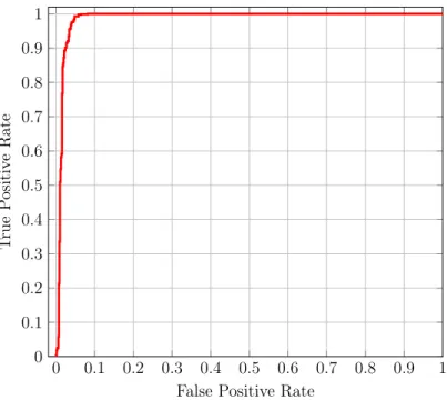
In machine learning, Receiving Operating Characteristics (ROC) is a graphical plot used to compute the Area Under the Curve (AUC) value and determine the efficiency of the algorithm. We generate the ROC curve by plotting the True Positive Rate (TPR) versus the False Positive Rate (FPR) with varying threshold through the range of data points. Figure 17 shows ROC curve with a shaded region. We compute the area of the shaded region to obtain the AUC value. This value usually lies in between 0.5 to 1. An AUC value of 1 indicates ideal classification with zero false positives or false negatives.

Figure 17: ROC curve with shaded area

(59)

by plotting ROC curve and calculating the AUC value.

6.4 SVM Model Experiments 6.4.1 Image Feature Statistics

The initial step of this method is to retrieve 21 image features. These features are adopted with the motivation that the spam image possesses different visual statistics compared to the genuine image. To demonstrate this, we first plotted the distributions for each of the 21 features in two distinct classes for dataset 1. The visualizations of the most effective features have been presented in Figure 18.

We can observe that the chosen features can certainly distinguish between the spam image and ham image. There is a clear mark of separation between the two classes of images. Further, we plotted the ROC curves to compute the AUC value for each of the features score obtained using SVM classifier. The ROC curves corre-sponding to the features in Figure 18 can be observed in Figure 19. It is apparent from the results that each feature by itself discriminates strongly between both the classes. The distributions and the ROC graphs for all the features are shown in the Appendix A.

Further we plot the AUC for all the 21 features for images from dataset 1 as shown in the Figure 20. We observe that the variances of different color channels produce a high classification rate. The color histogram based statistical features are most active in the exposition of the spam images. The analysis of the plot strengthens the fact that the spam image possesses properties that could be distinguished from the normal images. And, each feature individually could classify the images to a reasonable degree.

(60)

(a) Signal to noise ratio (b) Compression ratio

(c) LBP (d) Edge Count Figure 18: Feature distribution for spam versus ham images

6.4.1.1 Kullback-Leibler Divergence

We further computed the Kullback-Leibler divergence [21](known as KL diver-gence) for the probability distributions between the two classes of data for each fea-ture. KL divergence is a distance metrics that measures the difference between two probability distributions M and N. Concretely, the KL divergence of N from M is denoted by 𝐷𝐾𝐿(𝑀 ‖𝑁) and measures the amount of added information needed to

(61)

0 0.2 0.4 0.6 0.8 1 0 0.2 0.4 0.6 0.8 1 FPR TPR

(a) Signal to noise ratio

0 0.2 0.4 0.6 0.8 1 0 0.2 0.4 0.6 0.8 1 FPR TPR (b) Compression ratio 0 0.2 0.4 0.6 0.8 1 0 0.2 0.4 0.6 0.8 1 FPR TPR (c) LBP 0 0.2 0.4 0.6 0.8 1 0 0.2 0.4 0.6 0.8 1 FPR TPR (d) Edge Count Figure 19: ROC curves for the feature distributions in Figure 18

Figure 20: AUC for Feature distributions

(62)

𝐷𝐾𝐿(𝑀 ‖𝑁) =

∑︁

𝑖

𝑀(𝑖) log 𝑀(𝑖)

𝑁(𝑖), (11)

where M and N are discrete probability distributions [27]. KL divergence is non-symmetric, that is 𝐷(𝑀 ‖𝑁)is not equal to 𝐷(𝑁 ‖𝑀).

Using equation (11), we computed the KL divergence for the feature distributions from ham to spam and spam to ham. The results are given in the Table 4.

Table 4: KL divergence for Feature distributions

Feature Spam to Ham Ham to Spam SVM AUC

Color hist 0.01 0.01 0.58 Mean1 0 0 0.5 Mean2 0 0 0.5 Mean3 0 0 0.5 Var1 0.08 0.07 0.96 Var2 0.11 0.09 0.98 Var3 0.1 0.09 0.97 Skew1 0.23 0.23 0.91 Skew2 0.26 0.27 0.95 Skew3 0.22 0.28 0.94 Kurt1 0.32 0.29 0.92 Kurt2 0.35 0.33 0.94 Kurt3 0.31 0.36 0.94 LBP 0.01 0.01 0.85 HOG 0.04 0.03 0.81 Edge no 0.04 0.05 0.87 Edge len 0.02 0.02 0.65 Comp 0.04 0.01 0.95 Aspect 0.03 0.04 0.77 SNR 0.15 0.04 0.95 Noise 0.02 0.01 0.63