Ensemble methods in multi-label classification

Thesis presented in partial fulfilment of the requirements for the degree of

MCom (Mathematical Statistics) in the Faculty of Economic and Management Sciences at Stellenbosch University

The financial assistance of the National Research Foundation (NRF) towards this research is hereby acknowledged. Opinions expressed and conclusions arrived at, are those of the author

and are not necessarily to be attributed to the NRF.

December 2018

ii

Declaration

By submitting this thesis electronically, I declare that the entirety of the work contained therein is my own, original work, that I am the sole author thereof (save to the extent explicitly otherwise stated), that reproduction and publication thereof by Stellenbosch University will not infringe any third party rights and that I have not previously in its entirety or in part submitted it for obtaining any qualification.

Initials and surname Date

A Muller December 2018

Copyright © 2018 Stellenbosch University All rights reserved

iii

Abstract

There are many scenarios where several labels may be associated simultaneously with each data case in a dataset. Therefore, a large number of multi-label datasets are found in a variety of domains, including image annotation, text annotation, bioacoustics, music research and medical diagnostics. In this thesis, we focus on such multi-label datasets with the particular goal of performing label classification. Multi-label classification is an extension of binary- and multi-class multi-classification to scenarios where each instance in a dataset can have multiple or none of

K

labels.

Methods to perform multi-label classification can be divided into three categories: problem transformation methods, algorithm adaptation methods and multi-label ensemble methods. Multi-label ensemble methods receive particular attention in this research. We discuss previously proposed multi-label ensemble methods and also propose a new multi-label ensemble method, named label dependent splitting (LDsplit) with trees.

LDsplit with trees constructs an ensemble of tree-structures by considering different permutations of the labels in a multi-label dataset. The method differs from other multi-label ensemble methods since each tree-structure splits the multi-label data in a label-dependent way, whilst incorporating label correlation. Furthermore, each split of a node in a tree-structure is performed by considering a binary classification problem. By performing an empirical study on benchmark datasets, the predictive performance of LDsplit with trees is compared to that of other multi-label learning methods. LDsplit with trees produces very promising results, allowing us to believe that with further modifications the procedure may become a highly competitive multi-label learning method. Furthermore, we also explore aspects of analysing text data. We perform an extensive analysis on a practical multi-label text dataset. The practical dataset consists of online comments, where each comment is labeled to identify if any or multiple so-called “toxicity” are present in the comment. Our model may therefore be used to identify different types of toxicity present in online comments and help reduce online abuse and harassment. A particular challenge faced in the practical data analysis is the sparsity of the labels.

Keywords:

iv

Opsomming

Baie scenarios bestaan waar verskeie etikette gelyktydig met elke datageval in ‘n datastel geassosieer word. Daarom vind ons ‘n groot hoeveelheid multi-etiket datastelle in ‘n verskeidenheid van domeine, insluitend beeld-annotasie, teks-annotasie, bio-akoestieks, musieknavorsing en mediese diagnose. In hierdie tesis fokus ons op sulke multi-etiket datastelle met die spesifieke doel om multi-etiket klassifikasie uit te voer. Multi-etiket klassifikasie is ‘n uitbreiding van binêre- en multiklas klassifikasie na scenarios waar elke geval in ‘n datastel verskeie of geen van

K

etikette het.

Metodes wat gebruik word om multi-etiket klassifikasie uit te voer, kan in drie kategorieё verdeel word: probleem transformasie metodes, algoritme aanpassings metodes en multi-etiket ensemble metodes. Multi-etiket ensemble metodes kry spesifieke aandag in hierdie navorsing. Ons bespreek voorheen voorgestelde multi-etiket ensemble metodes en stel ook ‘n nuwe multi-etiket ensemble metode voor, genaamd etiket afhanklike splitting (LDsplit) met bome.

LDsplit met bome bou ‘n ensemble van boom-strukture deur verskillende permutasies van die etikette in die multi-etiket datastel te beskou. Die metode verskil van ander multi-etiket ensemble metodes aangesien elke boom-struktuur die multi-etiket data op ‘n etiket-afhanklike basis opdeel, terwyl etiket-korrelasie terselfdetyd geїnkorporeer word. Daarbenewens word elke splitsing van ‘n node in ‘n boom-struktuur uitgevoer deur ‘n binêre klassifikasie probleem te beskou. Met behulp van ‘n empiriese studie op standaard datastelle word die voorspellings-prestasie van LDsplit met bome vergelyk met dié van ander multi-etiket leermetodes. LDsplit met bome lewer baie belowende resultate, wat ons dus toelaat om te glo dat, met verdere aanpassings, mag die prosedure ‘n hoogs kompeterende multi-etiket leermetode word.

Verder verken ons ook aspekte van teksdata. Ons voer ‘n uitgebreide analise op ‘n praktiese multi-etiket teksdatastel uit. Die praktiese-datastel bestaan uit aanlyn kommentaar, waar elke individu se kommentaar gemerk word om vas te stel of enige of verskeie tipes toksisiteit teenwoordig is. Ons model kan dus gebruik word om verskillende tipes toksisiteit in aanlyn kommentaar te identifiseer en help om aanlyn misbruik en teistering te verminder. ‘n Besonderse uitdaging in die praktiese-data analise is die ylheid van die etikette.

Sleutelwoorde:

v

Acknowledgements

I hereby wish to acknowledge the Department of Statistics and Actuarial Science of Stellenbosch University for providing me with the necessary support to complete this thesis. I am also thankful for the South African Statistical Association National Research Foundation (SASA-NRF) grant. Finally, I wish to thank Professor S.J. Steel for supervising my research.

vi

Table of contents

Declaration ... ii Abstract ...iii Opsomming ...iv Acknowledgements ... v

Table of contents ...vi

List of figures ...ix

List of tables ...xi

List of appendices ...xii

List of abbreviations and/or acronyms ... xiii

CHAPTER 1: INTRODUCTION ... 1

1.1 CLASSIFICATION ... 1

1.2 EXAMPLES OF MULTI-LABEL DATASETS ... 2

1.2.1 Image annotation ... 3 1.2.2 Text annotation ... 3 1.2.3 Bioacoustics ... 4 1.2.4 Music ... 4 1.2.5 Medical diagnostics... 4 1.3 NOTATION ... 4 1.4 OVERVIEW ... 6

CHAPTER 2: MULTI-LABEL DATA ... 7

2.1 ASPECTS OF MULTI-LABEL DATA ... 7

2.1.1 Number of labels,

K

... 7 2.1.2 Label imbalance ... 7 2.1.3 Labelsets ... 8 2.1.4 Label correlation ... 8 2.1.5 Dimension reduction ... 8 2.1.6 Subsampling ... 9 2.1.7 Benchmark datasets ... 9

2.1.8 Synthetic data generation ...10

2.2 PERFORMANCE MEASURES ...11

vii

3.1 CATEGORIES ...15

3.2 BINARY RELEVANCE ...16

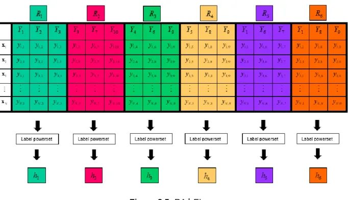
3.3 LABEL POWERSET ...17

3.4 CLASSIFIER CHAINS ...18

3.5 ENSEMBLES OF CLASSIFIER CHAINS ...22

3.6 RANDOM FORESTS OF PREDICTIVE CLUSTERING TREES ...24

3.7 RANDOM k-LABELSETS ...26

3.7.1 Description ...26

3.7.2 Performance ...33

3.7.3 Parameters ...34

CHAPTER 4: NEW APPROACH ...36

4.1 INTRODUCTION ...36

4.2 LDSPLIT WITH TREES ...36

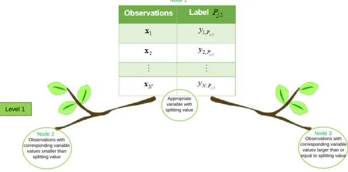
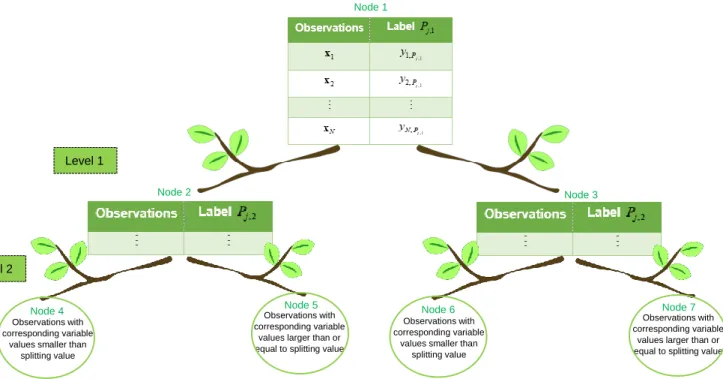
4.2.1 Fitting a tree-structure ...36

4.2.2 Issues regarding the tree-structure ...39

4.3 CLASSIFICATION ...42

4.3.1 Classification by means of a tree-structure ...43

4.3.2 Obtaining a final classification ...45

4.3.3 Using posterior probabilities ...45

4.4 ADAPTATION ...46

4.4.1 LDsplit with trees while

m



K

...46

4.4.2 Classification...48

4.5 EXPERIMENTAL EVALUATION OF LDSPLIT WITH TREES ...49

4.5.1 Experimental design ...51

4.5.2 Emotions ...53

4.5.3 Flags ...56

4.5.4 Yeast ...59

4.5.5 Conclusions ...60

4.6 CONCLUSION AND COMPARISON TO EXISTING METHODS ...61

4.6.1 Ensembles of classifier chains ...61

4.6.2 Random forests of predictive clustering trees...62

4.6.3 Random k-labelsets ...62

CHAPTER 5: PRACTICAL DATA ANALYSIS ...64

viii

5.1.1 Some approaches to organizing text data ...65

5.1.2 R packages ...67

5.2 MULTI-LABEL ANALYSIS IN R ...72

5.2.1 Package mldr ...72

5.2.2 Package mldr.datasets ...73

5.2.3 Package utiml ...74

5.3 PRACTICAL DATA ANALYSIS ...78

5.3.1 Initial cleaning and pre-processing ...78

5.3.2 Rude terms ...79

5.3.3 Top occurring terms ...80

5.3.4 Label inspection ...81 5.3.5 Feature selection ...89 5.3.6 Multi-label inspection ...96 5.3.7 Test data ... 100 5.3.8 Large data ... 100 5.3.9 Results... 101

CHAPTER 6: CONCLUSION AND OPPORTUNITIES FOR FUTURE RESEARCH ... 113

REFERENCES ... 118

APPENDIX A: Chapter 4 ... 121

A.1 FUNCTIONS FOR LDSPLIT WITH TREES ... 121

A.2 EMPIRICAL STUDY ... 136

APPENDIX B: Chapter 5 ... 145

B.1 LIST OF 174 STOPWORDS IN TM PACKAGE ... 145

ix

List of figures

Figure 1.1 Matrix representation of multi-label classification dataset

Figure 2.1 Categorization of performance measures for multi-label learning Figure 2.2 Confusion Matrix

Figure 3.1 Classification procedure of classifier chains for observation x Figure 3.2 Classification procedure for ensembles of classifier chains Figure 3.3 RA

k

EL_d

Figure 3.4 Prediction using RA

k

EL_d

Figure 3.5 RA

k

EL_o

Figure 3.6 Prediction using RA

k

EL_o

Figure 4.1 Representation of a stump fit to binary classification data Figure 4.2 Representation of tree-structure with two levels

Figure 4.3 Tree-structure with four levels

Figure 4.4 Summary of functions used for LDsplit with trees Figure 5.1 Representation of DTM

Figure 5.2 Representation of TDM Figure 5.3 Word cloud example Figure 5.4 Representation of DTM

Figure 5.5 Stacked column chart illustrating sparseness of labels Figure 5.6 Barplots of fifty top terms for each label

Figure 5.7 New barplots of fifty top terms for each label Figure 5.8 Word cloud for each label

x

Figure 5.10 Matrix representation of multi-label classification dataset Figure 5.11 Summary of mldr-object

Figure 5.12 Concurrence plot of mldr-object

Figure 5.13 Confusion matrices per learning method Figure 5.14 Label powerset with global threshold Figure 5.15 Label powerset with label-based threshold

Figure 5.16 Ensemble of classifier chains (Tree) with global threshold Figure 5.17 Ensemble of classifier chains (Tree) with label-based threshold Figure 5.18 Ensemble of classifier chains (Random Forest) with global threshold Figure 5.19 Ensemble of classifier chains (Random Forest) with label-based threshold

xi

List of tables

Table 2.1 Benchmark datasets

Table 3.1 Example of multi-label dataset

Table 3.2 Splitting multi-label data into binary classification data Table 3.3 Transformation of data in Table 3.1 to multi-class structure Table 3.4 Binary classification data of Table 3.1 used to find

f

₁

Table 3.5 Binary classification data of Table 3.1 used to find

f

₂

Table 3.6 Classifier chains applied to data in Table 3.1 Table 4.1 Summary of tree-structure levels

Table 4.2 Emotions data, LDsplit models with large

M

Table 4.3 Emotions data, LDsplit models with

K



M



2

K

Table 4.4 Emotions data model summary

Table 4.5 Flags data, LDsplit models with large

M

Table 4.6 Flags data, LDsplit models with

K



M



2

K

Table 4.7 Flags data model summary

Table 4.8 Yeast data, LDsplit models Table 4.9 Yeast data model summary

Table 5.1 R packages for base learners supported by the utiml package Table 5.2 Summary of R packages

xii

List of appendices

APPENDIX A Chapter 4

A.1 Functions for LDsplit with trees

A.2 Empirical study

APPENDIX B Chapter 5

B.1 List of 174 stopwords in tm package

xiii

List of abbreviations and/or acronyms

DTM Document-term-matrix

FN False negative

FP False positive

GUI Graphical user interface

HOMER Hierarchy of multilabel classifiers

LDsplit Label dependent splitting

MODT Multi-objective decision tree

NLP Natural language processing

PCorpus Permanent corpus

PCT Predictive clustering tree

RA

k

EL Random

k

−

labelsets

ROC Receiver operating characteristic

SMOTE Synthetic minority over-sampling technique

TDM Term-document-matrix

TN True negative

TP True positive

1

CHAPTER 1: INTRODUCTION

1.1 CLASSIFICATION

This thesis falls within the scope of supervised statistical learning, particularly, multi-label classification. In supervised statistical learning, a set of input variables, also known as predictors,

1, 2,..., p,

X X X are present along with output variables Y Y₁, ₂,...,Y_K. The output variables are also referred to as response variables. In supervised learning the goal is to fit a function,

1 2

( , ,..., _p) ( ) ,

f X X X = f X relating the input variables to the response variables. The training data can be denoted by:

{( ,

x y

_{i i}

),

i

=

1

, 2,...,

N

}.

Here

x

_i

,

i

=

1, 2,..., ,

N

denote

N

p

- component observations of input variables X X₁, ₂,...,X_p. The

K

-component response vectors

corresponding to the

N

observations are denoted by

y

_i

,

i

=

1, 2,..., .

N

The nature of the response variables,

Y Y

₁

,

₂

,...,

Y

_K

,

leads to the distinction between regression problems and classification

problems. If the response variables are numeric, i.e.

Y Y

₁

,

₂

,...,

Y

_K are quantitative, we refer to the prediction process of the response as a regression problem. If the response variables are specified in terms of classes, i.e.

Y Y

₁

,

₂

,...,

Y

_K are qualitative, we refer to the prediction of the class(es) to which an input vector belongs as a classification problem.

A common type of classification problem is binary classification. In the case of binary classification,

K

=

1

and

Y



 

0 ,1 .

In other words, there exists two disjoint classes, one class denoted by

Y

=

1

and the other class denoted by

Y

=

0.

If observation i is included in the first class this is denoted by letting

y

_i

=

1

and if observation i is included in the second class this is denoted by letting

y

_i

=

0.

A different way of viewing this is to let

K

denote the number of so called “labels”. Then, in the case of binary classification, where

K

=

1

, we have one label for the data. Then each observation either has this label present (denoted by

y

_i

=

1

) or does not have this label present (denoted by

y

_i

=

0

). Many classification problems resemble this form. For example, a dataset may consist of credit card transactions where each transaction is classified to be fraudulent or not. In this case, fraudulent transactions can be denoted by letting

y

_i

=

1,

and nonfraudulent transactions can be denoted by letting

y

_i

=

0.

Viewed differently, there is one label in this dataset, the “fraudulent”-label. Each observation either has this label present, i.e. the

2

transaction is fraudulent, denoted by

y

_i

=

1,

or does not have this label present, i.e. the transaction is not fraudulent, denoted by

y

_i

=

0.

In multi-class classification we have K=1and

Y





1, 2,...,

G



.

Here, each observation belongs to one of G classes and the G classes are disjoint. If the ith observation belongs to the

g

th

class, this can be denoted by letting

y

_i

=

g

where i=1,...,N and g=1,...,G. A multi-class classification problem can for example be the classification of handwritten digits. In this scenario, digits zero to nine denote the G=10 classes and each handwritten observation belongs to one of the ten classes.

In multi-label classification we have

K



1

and

Y

_k



 

1, 0

where k =1,..., .K Here each observation can have multiple or none of

K

labels. The labels are not disjoint. The

k

th entry of

i

y

equals 1 if the ith observation has the

k

th label present, where k=1,...,K and i=1,...,N.

Multiple entries of

y

_i can therefore equal 1 if observation i has multiple of the

K

labels present. It may also be that observation i has none of the labels present, in which case all the entries of

i

y

equal 0.

Finally, in multi-class multi-label classification,

K



1

and

Y

k





1,...,

G



where k =1,..., .K Now the

K

labels each consists of

G

disjoint label classes. This is arguably the most complex type of classification and is also sometimes referred to as multidimensional classification. In this thesis we focus on the slightly simpler classification type, namely multi-label classification in which case we have

K



1

and

Y

_k



 

1, 0

for k=1,..., .K

1.2 EXAMPLES OF MULTI-LABEL DATASETS

In the modern world where vast amounts of digital data have become the norm, many multi-label datasets can be found in a variety of fields. Some particular examples of multi-label dataset domains include image annotation, text annotation, bioacoustics, music and medical diagnostics. In this section we list a few of the large number of multi-label datasets found in a variety of domains. It is clear that multi-label data analysis has become an active area of research.

3 1.2.1 Image annotation

In image annotation, the data scientist can for example aim to supply tags to images on the internet. In this case, the

K

labels of the multi-label dataset correspond to

K

possible image-tags. Tags can for example include: sunset, mountain, beach, field, lighthouse, tower, etc. The training data of such an analysis consists of many internet images along with the appropriate tags that are present for each image. It may be useful for image search engines like Google Images or Pinterest to use the results of such a multi-label image analysis in order to improve search results for their users. Many multi-label classification image datasets can be found in practice. Another example is found on http://www.kaggle.com, an online data-sharing platform, hereafter referred to as Kaggle. Here, users are provided with a dataset containing a collection of movie posters along with the genres each movie falls into. The aim of the analysis is to build a classifier that can identify all the appropriate genres a movie falls into by only considering the movie poster. Each movie falls into one or multiple genres. Genres include: horror, romance, animation, comedy, etc. Here the data scientist might take note of the colours used on the posters, the brightness of the colours or the expressions of the actors on the posters, in order to find hints of the specific genres the movies fall into (Kaggle: Movie genre from its poster, 2018).

Multi-label image datasets are not only limited to still images. Observations in the form of video clips are also common. For example, a dataset found on Kaggle contains over 7 million YouTube videos along with 4716 video labels. A very large dataset indeed. The aim is to build a powerful classifier that can provide relevant video labels to new videos and by doing so improve the search and organization of video archives (Kaggle: Google Cloud & YouTube-8M video understanding challenge, 2017).

1.2.2 Text annotation

In text annotation it might be that the aim is to attach categories to text documents. Then the

K

labels of the multi-label dataset correspond to

K

possible text categories. Categories may include: biography, review, sport, food, blog or even “fake news”. A multi-label text dataset is also found on Kaggle: Greek media monitoring multi-label classification. The data consists of a number of Greek print media from May 2013 to September 2013, categorized to one or more topics by human annotators. Topics include specific persons, products or companies as well as more general topics such as economy and environment. The goal is to build a classifier that can identify the appropriate topics present for a new article. Some of the topics, such as specific persons, products or companies, might be easier to classify since they are based on keywords. Other

4

topics, such as environment or economy, might be more difficult to detect in an article since they are more general concepts (Kaggle: Greek media monitoring multi-label classification,2014).

1.2.3 Bioacoustics

In the bioacoustics domain, the data may for example consist of sound fragments and the aim may be to identify all the different bird species in each sound fragment. In this case, the

K

labels of the multi-label dataset correspond to

K

different bird species and the observations of this multi-label classification dataset are in the form of audio sound fragments.

1.2.4 Music

Another example of multi-label classification, where the observations may be in the form of audio fragments, is instrument recognition. Different types of musical instruments playing simultaneously can for example be identified in music pieces. The training data of such an analysis consist of many musical pieces along with the corresponding instruments present in each musical piece. Therefore the

K

labels in this multi-label dataset correspond to

K

musical instruments.

1.2.5 Medical diagnostics

In medical diagnostics, multiple medical conditions can be identified for a patient. For example, a dataset available on Kaggle contains 5606 chest X-ray images of patients and a total of 14

disease-labels. Diseases found in each of the X-ray images are labelled as such. Some X-ray images have no disease present, whereas others have one or multiple of the 14 disease-labels present. Additional information, such as the patient’s age and gender, are also available for each of the 5606 observations. Building a powerful classifier for such a multi-label dataset can improve diagnoses of these diseases for future patients (Kaggle: Random sample of NIH chest X-ray dataset, 2017).

1.3 NOTATION

In this thesis the multi-label classification data,

{( ,

x y

_{i i}

),

i

=

1

, 2,...,

N

},

are summarized as a

( )

N p+K matrix

.

N p N K









5

Input variables Label indicator variables

Data observations

X

₁

X

₂ Xp

Y

1

Y

2

Y

K

1 x1,1 x1, 2 x1,p 1

0

1

2 x2,1 x2, 2 x2,p

1

1 1

3

x3,1 x3, 2 x3,p 0 1 1

N

xN,1 xN, 2 xN p,

0

1

0

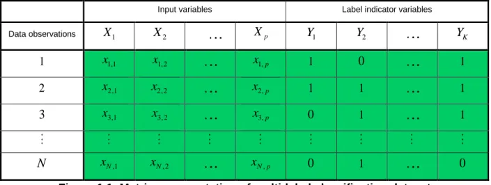
Figure 1.1: Matrix representation of multi-label classification dataset

Figure 1.1 consists of

N p

- component observations,

x

_i

,

i

=

1,..., ,

N

of the input variables

1, 2,..., p.

X X X There is a total of

K

labels denoted by

Y Y

₁

,

₂

,...,

Y

_K

.

Therefore, each observation

has a

K

- component label indicator resulting in a total of

N

K

-component label indicators,

,

1,..., ,

i

i

=

N

y

for the dataset. The first observation, for example, has both labels

Y

₁ and

Y

_K

present, the second observation has labels

Y

₁

,

Y

₂ and

Y

_K present and so on for all

N

observations. We denote the collection of labels,

Y Y

₁

,

₂

,...,

Y

_K

,

by L.

In some cases, the labels of a training dataset may be in the form of a hierarchical structure. This means that the labels are organized into general-to-specific levels. The top level of the hierarchy consists of a few general classes. Each of these classes in turn subdivide into slightly more specific classes, and these classes are in turn subdivided, and so on. The classification process of new observations in such a hierarchical structure is referred to as hierarchical classification. If observations are labelled with more than one node in the hierarchical structure, the classification process of a new observation is referred to as hierarchical multi-label classification (Tsoumakas and Katakis, 2007:3). In this thesis, the focus will however be on non-hierarchical multi-label classification. Therefore, when multi-label classification is mentioned, we are in fact referring to non-hierarchical multi-label classification.

Our goal in the multi-label analysis is multi-label classification. We thus aim to fit a function relating the input variables to the labels, with the goal of using this fitted function to classify an unseen observation to relevant labels as accurately as possible. Inference may also be a goal of a multi-label analysis. Understanding the relationship between different multi-labels and different variables are

6

often of interest. In medical diagnostics, for example, it can be very advantageous if an analysis reveals which predictors are correlated with which medical conditions. Another multi-label analysis goal worth mentioning is multi-label ranking. In the case of multi-label ranking, the aim is to fit a function relating the input variables to the labels, with the goal of using this fitted function to provide an unseen observation with a preference list, i.e. a ranking of the labels from the set of possible labels (Madjarov et al.,2012). Multi-label ranking is also an important topic in multi-label data analysis. An image search engine, for example, does not only provide users with relevant images when a search is carried out, but also provides users with a ranking of the images. Here the intention is that the first image presented to the user corresponds better to the user’s preference than those images that appear after it.

1.4 OVERVIEW

This thesis consists of six chapters. The first is an introductory chapter where we distinguish multi-label classification from other classification types. We also refer to some examples of multi-multi-label dataset domains, state our multi-label analysis goal and introduce the notation used for multi-label data in this thesis.

After multi-label data are introduced in the introductory chapter, Chapter 2 refers to unique characteristics of multi-label data compared to other data structures. Performance measures for multi-label data are also given.

Multi-label learning methods are discussed in Chapter 3. We outline the three categories of multi-label learning and state that multi-multi-label ensemble methods receive particular attention in this thesis. Three multi-label ensemble methods are discussed in this chapter.

In Chapter 4 we explain a new multi-label ensemble method. The predictive performance of this method is compared to that of previously proposed multi-label learning methods by performing a benchmark dataset analysis. We also highlight the key differences between the new approach and previously proposed multi-label ensemble methods discussed in this thesis.

In Chapter 5 our focus shifts to multi-label text data. We briefly discuss aspects of analysing text data and refer to useful R packages for text and multi-label analyses. The chapter concludes with a practical multi-label text data analysis. We describe the cleaning and pre-processing of the data, the feature selection process and multi-label characteristics of the data. Lastly, we present and discuss the results obtained when performing multi-label classification.

7

CHAPTER 2: MULTI-LABEL DATA

2.1 ASPECTS OF MULTI-LABEL DATA

Multi-label datasets have some unique characteristics compared to other data structures. Some of these aspects might influence the performance of different multi-label learning methods and are thus important to take note of. Other aspects might also make the analysis of a multi-label dataset more difficult. In this section we therefore briefly discuss some of these unique aspects, including: the value of K, label imbalance, labelsets, label correlation, dimension reduction, subsampling, benchmark datasets and synthetic generation of multi-label data.

2.1.1 Number of labels,

K

Some multi-label datasets have a very large number of labels,

K

.

The high dimensionality of datasets of this form can significantly influence the performance of multi-label methods. Some multi-label methods have a significant increase in computational cost if the number of labels is very large and for this reason are simply an inappropriate choice for datasets with large

K

.

Examples of domains with large numbers of labels include text categorization, protein function classification and semantic annotation of multimedia (Tsoumakas et al.,2008). The hierarchy of multilabel classifiers (HOMER) algorithm, described in Tsoumakas et al.(2008), is one example of a procedure developed to deal with this aspect of multi-label data.

2.1.2 Label imbalance

Another characteristic is the number of observations annotated with each label in the dataset. Sometimes the labels in a multi-label dataset can be imbalanced. Some labels may occur multiple times, i.e. the labels are present for many observations, whereas other labels may occur rarely,

i.e. the labels are present for very few of the observations. Learning methods trained on such imbalanced labels might struggle to identify new observations which have the less dominant labels present, since observations of this kind are so sparse in the training data. On the other hand, if

K

is very large, each observation might only have a few of the large number of labels present. In other words, all the labels are sparse. The average number of labels of the observations in the multi-label dataset is defined as label cardinality and is given by

1 1 . N i N i cardinality =

=



y Here,

y

_i denotes the number of entries in

y

_i that are equal to 1, i.e. the total number of labels observation i has present. The label density of a multi-label dataset is the

8

average number of labels of the observations divided by K, thus 1 1 . i N N K i density = =



y Label density therefore also takes the number of labels in the dataset into consideration. Two datasets may have the same cardinality but can differ significantly with regard to density. This can cause the two datasets to behave differently when the same multi-label learning method is applied (Tsoumakas and Katakis, 2007:8). The interested reader may also consult Charte and Charte (2018) for a definition of the so-called “imbalance ratio”, IRLbl.

2.1.3 Labelsets

The number of distinct label combinations per observation found in the dataset, i.e. the number of labelsets, may also influence the performance of multi-label methods. Some multi-label learning methods make specific use of the different labelsets in the learning process so that a large number of labelsets can significantly increase computational cost.

2.1.4 Label correlation

In multi-label analyses we might also consider label correlation. For example, we might ask which labels in the multi-label dataset are interdependent? Aspects of label correlation are useful for both inference and classification of unseen observations. Some labels in a multi-label dataset may have strong interdependencies. For a dataset like this, learning methods that try to exploit label dependencies may be a better choice than learning methods that do not try to exploit label dependencies. However, learning methods that incorporate label dependencies may be more computationally intensive, especially for large datasets. A simpler method might be faster, but has the disadvantage of possibly ignoring important information contained in the dataset. We discuss both types of learning methods in later chapters.

2.1.5 Dimension reduction

Some multi-label datasets have a large number of predictors. A wide variety of studies are dedicated to the topic of dimension reduction for single-label classification, where

K

=

1.

In the case of multi-label classification, where K1, various ad hoc approaches for variable selection have been proposed. Approaches for multi-label dimension reduction still pose an avenue for further research. The challenge is that

X

₃ can, for example, assist in predicting

Y

₁

,

but also make

predicting

Y

₂ more difficult. In other words, what determines the importance of a predictor in the multi-label classification scenario? A predictor has global importance when the predictor is globally correlated with all the labels, but some predictors are locally important in which case the

9

predictor is correlated only with a subset of the labels. Some approaches to multi-label variable selection include the filter approach, wrapper approach and the embedded approach, as outlined in Spolaôr et al.(2013).

2.1.6 Subsampling

When multi-label data are subsampled, as in the case of

k

−

fold cross-validation for example, the division is slightly more difficult compared to single-label data. In the multi-label case, we would like the proportion of observations per label in each subset to be approximately equal to that of the complete dataset. Randomly splitting the multi-label data into

k

folds will probably not allow this to be true. This is not ideal. For one or more of the folds it can for example happen that none of the observations are annotated with a rare label, or some labels may be overrepresented in some folds and completely underrepresented in others. Ideally the

k

folds should act as smaller versions of the complete dataset, having similar characteristics. Sechidis et al. (2011) outline stratification in the context of multi-label data. One approach focusses on distinct labelsets and the other considers each label independently of the rest.

2.1.7 Benchmark datasets

When research is carried out in the field of multi-label classification, researchers often make use of common multi-label benchmark datasets. The benchmark datasets are openly available to researchers. Analyses from different research papers can therefore be compared when the same benchmark datasets are used. The datasets belong to different domains, including music, images, text, etc. Table 2.1 summarizes some benchmark datasets used in multi-label research.

Table 2.1: Benchmark datasets

Dataset Domain

N

p

K

Label

cardinality Label density Emotions Music

593

72

6

1.87

0.311

Flags Image

₁₉₄

19

7

3.39

0.485

Scene Image

2407

294

6

1.07

0.179

Tmc2007 Text

28596

49060

22

2.16

0.098

Yeast Biology

₂₄₁₇

103

14

4.24

0.303

10

The Emotions dataset consists of

593

music-piece observations. Each music piece is labelled with a selection of six possible emotions namely: sad-lonely, angry-aggressive, amazed-surprised, relaxing-calm, quiet-still and happy-pleased. The Flags dataset consists of

194

flags and 19 flag features. Each flag is annotated with up to seven colours. The Scene dataset contains

2 407 images annotated with up to six concepts such as beach, mountain and field. The Tmc2007

dataset gives aviation safety reports that document problems that occurred during certain flights as observations. The labels of the Tmc2007 dataset are the problems being described by the reports. The Yeast dataset consists of 2 417 genes and each gene can be associated with 14 biological functions, so that the biological functions form the 14 labels of the Yeast dataset.

2.1.8 Synthetic data generation

When new multi-label learning methods are introduced, the benchmark datasets can be useful to investigate the performance of the newly introduced method against other learning methods. The benchmark datasets are also useful when properties of multi-label datasets are investigated. These datasets are useful, but they are not entirely sufficient. The “truth” of the benchmark datasets are unknown to researchers. For example, it is unknown which labels are correlated, which predictors are correlated or what the relationship between the labels and the predictors in the benchmark datasets are. Researchers generate synthetic data in order to have control and precise knowledge of such properties in investigations. In single-label classification, it is simple to systematically generate synthetic single-label classification data. It is however much more difficult to simulate synthetic multi-label data. In the case of multi-label analysis, we would like to incorporate multi-label characteristics, like those mentioned in this section, into the data. For example, the generated data should consist of

K

correlated binary labels as well as

p

input vectors of a specified multi-variate distribution. We would like the input vectors to depend on the labels in some way. We would also for example like some predictors to be good at predicting a certain label while simultaneously being bad at predicting another label. These issues make systematic generation of multi-label data more difficult. Few proposals exist for systematically generating synthetic multi-label data and this may still be a field that requires further research. Tomás et al. (2014) has contributed by proposing Mldatagen, a multi-label dataset generator framework. Other contributors include Sandrock and Steel (2017) proposing an algorithm that offers users the option to specify many aspects regarding the data to be generated.

11 2.2 PERFORMANCE MEASURES

Some of the above-mentioned aspects may influence the performance of different multi-label methods, but how can the performance of different label methods be measured? The multi-label data structure requires different performance measures from those used in traditional single-label classification. However, a large number of evaluation measures have been proposed for multi-label data. Measures exist for the evaluation of both multi-label classification as well as multi-label ranking. The following discussion is based on Tsoumakas et al. (2010).

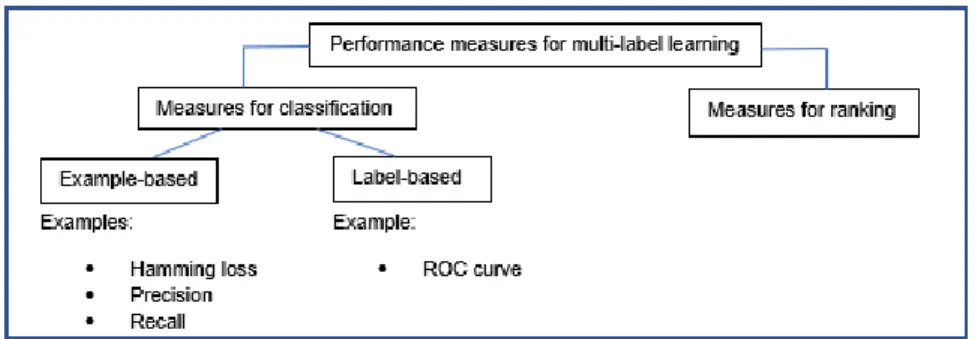
For multi-label classification, evaluation measures can be grouped into two main categories: example-based and label-based measures. As the name suggests, example-based measures consider each observation individually and computes the metric for each. The final performance value is obtained by averaging the performance values for the individual observations. Label-based metrics on the other hand consider each label individually and computes the metric for each label, instead of each observation. Figure 2.1 outlines the categorization of performance measures for multi-label learning.

Figure 2.1: Categorization of performance measures for multi-label learning

Consider a test dataset,

{( ,

x y

_{i i}

),

i

=

1

, 2,...,

M

},

and suppose our multi-label classifier gives classifications

f

( )

x

i

=

z

i

,

i

=

1,...,

M

,

where

 

0,1

.

K i



z

Some example-based measures

include the following. For a single test case, Hamming loss is the proportion of incorrectly predicted labels. Therefore, for the test data, Hamming loss is defined as:

1 1 1 . M K m k m k KM m k y z = = −



12

Precision on the other hand is given by:

1 1 1 1

.

K m k m k M k M K m m k k

y

z

precision

z

= = =













=

_

_



















Due to the way precision is defined, it produces an average proportion of those labels predicted to be present

(

Z

=

1

)

and which are correctly predicted, i.e. the label is in fact present

(

Y

=

1 ,

)

provided the denominator is not zero.

Recall is defined as:

1 1 1 1

.

K m k m k M k M K m m k k

y

z

recall

y

= = =













=

_

_



















Recall is the average proportion of true labels, i.e. labels that are present

(

Y

=

1 ,

)

which are predicted to be present

(

Z

=

1 ,

)

provided the denominator is not zero.

Precision and recall can also be combined into a single measure which is referred to as the F-score. The F-score is defined as:

2 . precision recall F precision recall   = +

Precision and recall are related to the concepts of sensitivity and specificity. Consider the confusion matrix given in Figure 2.2. Two types of incorrect classifications can be made by a multi-label classifier. If a label is present, i.e. Y =1, the classifier can predict the label not to be present, i.e. Z =0. This type of error is referred to as a false negative (FN) classification. On the other hand, if a label is not present, i.e. Y =0, the classifier can predict the label to be present,

i.e. Z =1. This type of error is referred to as a false positive (FP) classification. When a label is present, i.e. Y =1, and it is predicted to be present, i.e.

Z

=

1,

we refer to the classification as a true positive (TP) classification. When a label is not present, i.e. Y =0, and it is predicted not to be present, i.e. Z =0, we refer to the classification as a true negative (TN) classification.

13

Considering the total number of all these different classifications for a dataset, sensitivity is defined as TP

TP FN+ and specificity is defined as

.

TN

FP TN+ Precision is also given by TP FPTP+ and recall

is defined in the same way as sensitivity, i.e. TP

.

TP FN+ A trade-off exists between precision and

recall, with equality when

FP

=

FN

.

True label P red ict ed l ab el

1

Y

=

Y

=

0

1

Z

=

True Positive (TP) False Positive (FP)

0

Z

=

False Negative (FN) True Negative (TN)

Figure 2.2: Confusion Matrix

A label-based measure, on the other hand, can be any known evaluation measure for binary classification. The TP and FP rates for a single label can for example be used to construct a curve referred to as the receiver operating characteristic (ROC) curve. With TP rate given on the y-axis and FP rate given on the x-axis, the curve is traced out by varying the threshold value of the classifier. The overall performance of the classifier is given by the area under the ROC curve. The larger the area, the better the performance of the classifier, so that an ideal ROC curve hugs the top left corner of the graph. R packages that allow users easy comparison of the areas under the ROC curves and plotting of these curves include ROCR and pROC (Robin et al.,2011).

14

Denote by

TP

_k

,

TN

_k

,

FP

_k and

FN

_k the number of true positive, true negative, false positive and

false negative classifications after binary evaluation of label

k

.

Then, if a binary evaluation measure, calculated based on the number of TP, TN,

FP

and

FN

classifications, is denoted

by

B TP TN FP FN

(

,

,

,

)

,

the so-called macro-averaged and micro-averaged versions of

B

are given by:

(

)

1 1 , , , K macro K k k k k k B B TP TN FP FN = =



and 1 1 1 1 , , , . K K K K micro k k k k k k k k B B TP TN FP FN = = = =   =   











A multi-label learning method usually performs differently for different performance measures (Wu and Zhou, 2016). Therefore, multiple multi-label performance measures are used in a multi-label analysis.

This chapter highlights different challenges faced when analysing multi-label datasets. It is clear that single-label datasets and multi-label datasets cannot be approached in the same way. The multi-label data structure has some unique characteristics and requires specific tools in the analysis of the dataset, including the evaluation measures used when analysing predictive performance. In the next chapter multi-label learning methods are discussed. These learning methods are also particularly developed to handle the multi-label data structure.

15

CHAPTER 3: MULTI-LABEL LEARNING METHODS

3.1 CATEGORIES

In this chapter specific learning methods for label classification are discussed. Several multi-label learning methods exist. Initially, Tsoumakas and Katakis (2007) grouped these learning methods into two main categories: algorithm adaptation methods and problem transformation methods. In more recent years, multi-label learning methods have also been extended to a third category, namely multi-label ensemble methods.

Algorithm adaptation methods start with a previously defined single-label learning algorithm and aim to transform the algorithm to handle the multi-label data directly. Some examples of such algorithms that have been extended to the multi-label structure are decision trees, boosting, neural networks, support vector machines and

k

-nearest neighbours. The interested reader may consult Madjarov et al.(2012) for detailed descriptions of the adaptations.

Problem transformation methods are methods that use a single-label classification method (i.e.

multi-class or binary) for the multi-label data analysis. Usually the multi-label data are transformed in a specified way so that a single-label classification method can be applied. The multi-label learning problem is therefore split into one or more single-label classification problems. One single-label classification method is normally applied to the transformed data and the output is combined in a particular way so that the results have a multi-label structure. Many problem transformation methods exist. We highlight three problem transformation methods, namely binary relevance, label powerset and classifier chains. These three methods are sometimes used as base classifiers in other multi-label learning methods, we therefore highlight them in particular. In this thesis, the main focus will be on the third group of learning methods for multi-label data, namely ensemble methods. Ensemble schemes use several function estimates or predictions and combine them in a specified way in order to build one powerful, in our case, classifier. The base classifiers of these ensemble methods in our context belong to either of the two previously mentioned categories of multi-label methods, i.e. algorithm adaptation and problem transformation methods. Examples of ensemble methods for multi-label classification are ensembles of classifier chains in Read et al. (2011), random forests of predictive clustering trees in Kocev et al.(2007) and random

k

−

labelsets (Tsoumakas et al.,2011).

16 3.2 BINARY RELEVANCE

One of the simplest problem transformation methods is known as binary relevance. The following discussion is based on Tsoumakas and Katakis (2007). For illustration, consider the multi-label dataset given in Table 3.1 that contains

N

=

5

observations,

x

_i

,

i

=

1,...,5,

and

K

=

4

labels, denoted by

Y

_k

,

k

=

1,..., 4.

Table 3.1: Example of multi-label dataset

Input variables Label indicator variables

1

Y

Y

₂

Y

₃

Y

₄ 1

x

1

0

0

1 2

x

0

0

1 1 3

x

1

0

0

0

4

x

0

1 1

0

5

x

1 1 1

0

A problem transformation method transforms the multi-label data, such as that given in Table 3.1, so that a single-label classification method can be applied. In the case of binary relevance, the multi-label data are transformed by considering the data as

K

separate binary classification problems, one for each label. First an appropriate base classifier is chosen that can handle standard binary classification problems. Examples of such classifiers include linear discriminant analysis, logistic regression and support vector machines. We then fit

K

binary classification models, one for each label, using the base classifier. This results in

f

_k

,

k

=

1,...,

K

,

where

( )  

:

0;1 ,

1,...,

.

k k

f

x

→

Y

x



k

=

K

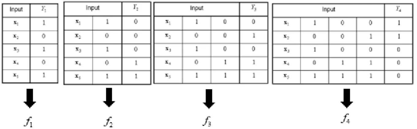
For the data in Table 3.1, this would mean that the multi-label data are divided into

K

=

4

separate binary classification problems, similar to Table 3.2. The base classifier is applied to each of the

K

=

4

binary classification versions of the data and

,

1,..., 4,

k

17 Table 3.2: Splitting multi-label data into binary classification data

1

Y

Y

₂

Y

₃

Y

₄ 1

x

1

x

1

0

x

1

0

x

1 1 2

x

0

x

2

0

x

2 1

x

2 1 3

x

1

x

3

0

x

3

0

x

3

0

4

x

0

x

4 1

x

4 1

x

4

0

5

x

1

x

5 1

x

5 1

x

5

0

Suppose we aim to classify an unseen observation,

x

.

In binary relevance, the

K

functions,

,

1,..., ,

k

f

k

=

K

are applied to the unseen observation, resulting in a separate classification for each of the

K

labels. For the data in Table 3.1, this would mean that the unseen observation, x,

is classified by _f₁

( )

x f₂

( )

x f₃

( )

x f₄

( )

x _.

The main advantages of binary relevance are that it is a simple and fast procedure. Unfortunately, binary relevance does not take label correlation into consideration. Each label prediction is made separately from the other labels and no label interactions are used in the binary relevance procedure.

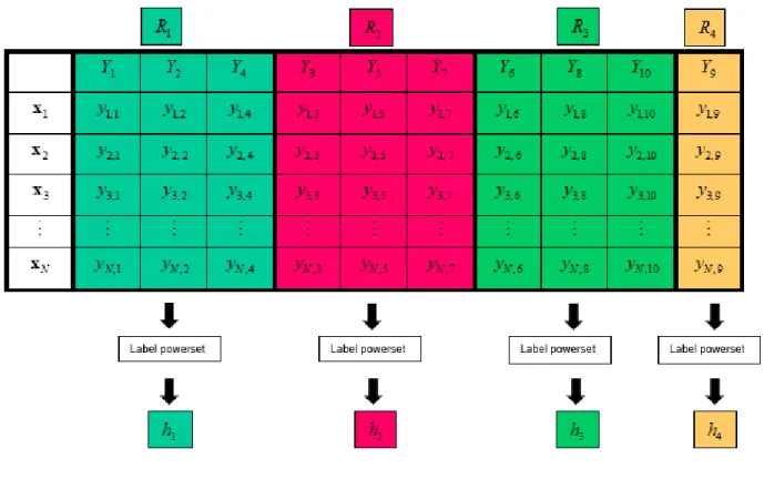
3.3 LABEL POWERSET

This section is based on Tsoumakas et al. (2011). The label powerset method is a problem transformation method that attempts to take label correlation into consideration. The label powerset approach recognizes each unique set of labels that exists in the multi-label dataset as a class. The multi-label data are therefore transformed to a multi-class structure. Applying this idea to the data in Table 3.1 causes the data to resemble Table 3.3. A standard multi-class classifier can then be applied to the multi-class version of the data. This multi-class classifier can then be used to classify an unseen observation by classifying the observation to the class with the highest posterior probability.

18 Table 3.3: Transformation of data in Table 3.1 to multi-class structure

1

Y

Y

₁ and

Y

₄

Y

₁

,

Y

₂ and

Y

₃

Y

₂ and

Y

₃

Y

₃ and

Y

₄

1

x

0

1

0

0

0

2

x

0

0

0

0

1 3

x

1

0

0

0

0

4

x

0

0

0

1

0

5

x

0

0

1

0

0

Unfortunately, the label powerset method can only classify an unseen observation to a labelset present in the training data. This limits the procedure since no new label combination can be formed. New label combinations, not found in the training dataset, can easily occur in test datasets. This property of the label powerset method may cause an increase in its test error. The label powerset procedure also has the disadvantage that the transformation of the multi-label data to a multi-class structure may lead to a dataset with a large number of classes and few observations per class. This is especially true for multi-label datasets that have a large number of labels. The total number of possible labelsets for a multi-label dataset, and therefore also the total number of possible classes for the multi-class version of the data, is upper bounded by

(

)

min N, 2K . In practice, the number is normally much smaller than the upper-bound, however it can still be large enough to make the learning process difficult. Depending on the multi-class classification algorithm used in the label powerset procedure, a large number of labelsets may significantly increase computational cost. Furthermore, with few observations per class in the multi-class version of the data, the learning process becomes more difficult so that the fitted model may not perform so well on test data.

3.4 CLASSIFIER CHAINS

The classifier chains approach is a problem transformation method based on the binary relevance method. The method aims to improve on some of the shortcomings of the binary relevance method, while retaining the advantages of being simple and fast. The following discussion is based on Read et al. (2011).

19

The main disadvantage of binary relevance that the classifier chains method aims to improve, is the fact that binary relevance does not take label correlation into consideration. In binary relevance,

K

binary classification models,

f

_k

,

k

=

1,..., ,

K

are fit separately, one for each label. Classifier chains also applies

K

binary transformations that result in

K

classifiers,

,

1,..., .

k

f

k

=

K

However, when fitting classifier chains, the input space of each binary model is extended with the

0 / 1

label relevance of all previous classifiers. The procedure is therefore appropriately named, since a chain of classifiers is indeed formed.

Suppose a multi-label classification dataset,

{( ,

x y

_{i i}

),

i

=

1

, 2,...,

N

},

is given consisting of

N p

- component observations of input variables X₁,...,X_p and a total of

K

labels,

Y Y

₁

,

₂

,...,

Y

_K

.

After

an appropriate base classifier that can handle standard binary classification problems is chosen, the classifier chains method is implemented as follows.

The first binary classifier,

f

₁, is found by fitting the base classifier to the binary classification data

formed by considering

x

₁

,...,

x

_N

,

along with the

N

response entries of the first label. Considering

the data in Table 3.1 as an example, we therefore fit the base classifier to the binary classification data given in Table 3.4, in order to find

f

₁

.

Table 3.4: Binary classification data of Table 3.1 used to find

f

₁

Input

Y

₁ 1

x

1 2

x

0

3

x

1 4

x

0

5

x

1

In order to obtain the second binary classifier,

f

₂

,

the input variables become



X₁,...,X_p



 

Y₁ .

20

considering the

N

observations of the input variables



X₁,...,Xp



 

Y₁ , along with the

N

response entries of the second label. Considering the data in Table 3.1, we therefore fit the base classifier to the binary classification data given in Table 3.5 to find

f

₂

.

Table 3.5: Binary classification data of Table 3.1 used to find

f

₂

Input

Y

₂ 1

x

y1,1=1

0

2

x

y2,1=0

0

3

x

y3,1=1

0

4

x

y4,1=0 1 5

x

y5,1=1 1

In general,

f

_k is trained using input variables



X₁,...,Xp





Y₁,...,Yk−₁



and the response entries

of the kth label. Here k=1,...,K so that a chain of

K

classifiers is formed,

f

=

(

f

₁

,...,

f

_K

)

.

Again consider the data in Table 3.1 as an example. In this case we find a chain of

K

=

4

classifiers by fitting the base classifier to each of the four binary classification datasets given in Table 3.6.

21

Once the chain,

f

,

is complete, containing

K

classifiers, the classification of an unseen

observation, x, can be made. Starting at

f

₁ we find the

0 / 1 classification,

f x

ˆ

1

( )

.

Then the

second binary classifier,

f

₂

,

predicts the relevance of the second label, given the input space

augmented by the

0 / 1 value,

f x

ˆ

1

( )

.

In general, the

th

k binary classifier predicts the relevance of the kth label, given the input space augmented by the

0 / 1 classifications of all the previous

binary classifiers in the chain. This is illustrated in Figure 3.1.

Input

_{0 / 1}

classification 1

x

x

₂ xp

f x

ˆ

1

( )

1

x

x

₂ xp

f x

ˆ

1

( )

f

ˆ

2

( )

x

1

x

x

₂ xp

f x

ˆ

1

( )

f

ˆ

2

( )

x

f x

ˆ

3

( )

1

x

x

₂ xp

f x

ˆ

1

( )

f

ˆ

2

( )

x

f

ˆ

K−1

( )

x

f

ˆ

K

( )

x

Final classification

Y

₁

Y

₂

Y

_K

( )

ˆ

₌

f x

f x

ˆ

₁

( )

f

ˆ

₂

( )

x

f

ˆ

_K

( )

x

Figure 3.1: Classification procedure of classifier chains for observation x

Since the classifier chains method passes label information between classifiers, it incorporates label correlation and overcomes the disadvantage of binary relevance of not taking label correlation into consideration. Read et al. (2011) state that although the additional attributes make up a small part of the total attribute space, if strong correlations exist, these attributes give any base classifier relatively more predictive power.

Note that only one ordering of the

K

labels is used in the classifier chains method. This is a possible disadvantage of classifier chains. Predictive performance of the fitted classifier chains

22

model is very dependent on the order of the chain, i.e. the order of the labels

Y

₁

,...,

Y

_K

,

it was trained on. It may happen that one or more of the first classifiers in the chain classify poorly, which means that the classifiers later in the chain use these poor classifications to find a classification for the labels that occur later in the chain. This concern may be addressed by considering an ensemble of classifier chains, which is described in the next section.

3.5 ENSEMBLES OF CLASSIFIER CHAINS

Instead of considering only one ordering of the

K

labels, as is the case for the classifier chains method, the ensemble of classifier chains method considers multiple orderings of the

K

labels and fits an ensemble of classifier chains. This multi-label ensemble method, given in Read et al. (2011), is described in this section.

Again consider a multi-label classification dataset,

{( ,

x y

_{i i}

),

i

=

1

, 2,...,

N

}.

It is straightforward to fit an ensemble of classifier chains. Instead of considering only one order of the labels to form one chain, f, we consider

m

random orderings of the

K

labels in order to fit

m

classifier chains,

1

,...,

m

.

f

f

Each classifier is trained on a bootstrap sample formed by sampling

N

times with

replacement from the observations in the multi-label training dataset. Therefore, along with the

m

random orderings of the

K

labels,

m

bootstrap samples of the multi-label classification training dataset are required to fit

m

classifier chains,

f

₁

,...,

f

_m

.

It was initially suggested, in Read

et al. (2009), to use a subset of the observations in the training dataset to fit each classifier. Thus, sampling without replacement in this case. However, it was discovered that using bootstrap samples can achieve higher predictive performance with only a small increase in computational cost. We therefore focus on the bootstrap implementation of ensembles of classifier chains in our description of the method.

To form the first classifier,

f

₁

,

the

N

p

−

component observations of the first bootstrap sample are considered along with their corresponding response entries of the

K

labels. Using these

N

observations and the first random label ordering, a classifier chain is fit as described in Section 3.4. This produces

f

₁

.

In order to find the second classifier, we consider the second bootstrap sample observations along with the second random label ordering and fit a classifier chain. This produces

f

₂

.

We continue in this way until

m

multi-label classifiers,

f

₁

,...,

f

_m

,

have