2014
Mixed effects modeling with missing data using
quantile regression and joint modeling
Luke Karsten Fostvedt
Iowa State UniversityFollow this and additional works at:
http://lib.dr.iastate.edu/etd
Part of the
Education Commons, and the
Mathematics Commons
This Dissertation is brought to you for free and open access by the Graduate College at Digital Repository @ Iowa State University. It has been accepted for inclusion in Graduate Theses and Dissertations by an authorized administrator of Digital Repository @ Iowa State University. For more
information, please [email protected].
Recommended Citation
Fostvedt, Luke Karsten, "Mixed effects modeling with missing data using quantile regression and joint modeling" (2014).Graduate Theses and Dissertations.Paper 14153.
modeling
by
Luke Karsten Fostvedt
A dissertation submitted to the graduate faculty in partial fulfillment of the requirements for the degree of
DOCTOR OF PHILOSOPHY
Major: Statistics
Program of Study Committee: Mack C. Shelley II, Major Professor
Dianne Cook Daniel Nordman W. Robert Stephenson
Wolfgang Kliemann
Iowa State University Ames, Iowa
2014
DEDICATION
TABLE OF CONTENTS LIST OF TABLES . . . vi LIST OF FIGURES . . . ix ABSTRACT . . . xi CHAPTER 1. OVERVIEW . . . 1 1.1 Linear Models . . . 3
1.1.1 Linear Mixed Effects Models . . . 3
1.1.2 Multivariate Linear Mixed Effects Models . . . 4
1.1.3 Contribution . . . 5
1.2 Quantile Regression . . . 6
1.2.1 Modeling Longitudinal Data . . . 7
1.2.2 Recursive Structural Equation Modeling . . . 10
1.2.3 Missing Data . . . 10
1.3 The Future of Quantile Regression . . . 11
1.3.1 Contribution . . . 11
CHAPTER 2. EFFECT OF CORRELATION ON THE ESTIMATION OF MULTIVARIATE MIXED EFFECTS MODELS . . . 13
2.1 Introduction . . . 14
2.2 Model . . . 15
2.2.1 Estimation via the Expectation-Maximization Algorithm . . . 17
2.3 Simulations . . . 18
2.3.1 Hierarchical Models . . . 18
2.4 Results . . . 21
2.5 Education Example . . . 23
2.5.1 Model and Results . . . 25
2.6 Discussion . . . 28
2.6.1 Contribution and Further Work . . . 28
2.7 Appendix . . . 28
CHAPTER 3. MULTI-LEVEL QUANTILE REGRESSION . . . 56
3.1 Introduction . . . 57
3.2 Bayesian Quantile Regression . . . 58
3.2.1 Modeling . . . 59 3.3 Education Intervention . . . 60 3.4 Results . . . 62 3.5 Discussion/Conclusion . . . 63 3.6 Appendix . . . 65 3.7 Derivations . . . 71
CHAPTER 4. DATA IMPUTATION IN MULTI-LEVEL QUANTILE RE-GRESSION WITH AN APPLICATION TO PISA 2012 RESULTS . . . . 74
4.1 Introduction . . . 75
4.1.1 Missing Data Mechanisms . . . 76
4.2 Quantile Regression and Missing Data . . . 77
4.2.1 Population Model . . . 77
4.2.2 Missing Data Modeling . . . 79
4.3 Simulations . . . 80
4.3.1 Generating Missing Values . . . 80
4.3.2 Hierarchical Data . . . 81
4.3.3 Results . . . 82
4.4 Example: PISA 2012 . . . 83
4.6 Appendix . . . 91
CHAPTER 5. SUMMARY AND DISCUSSION . . . 108
5.1 Simultaneous Inferences . . . 108
5.2 Missing Data in Quantile Regression . . . 109
5.3 Multi-level Quantile Regression . . . 110
LIST OF TABLES
Table 2.1 Science Scores . . . 26 Table 2.2 Reading Scores . . . 26 Table 2.3 Math Scores . . . 27 Table 2.4 Comparison of variances between univariate and joint modeling . . . . 27 Table A2.1 Average estimates of the fixed effects and the standard errors from 100
simulations of a two-level hierarchical model. . . 29 Table A2.2 Average estimates of the fixed effects and the standard errors from 100
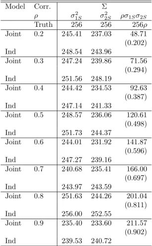
simulations of a two-level hierarchical model. . . 30 Table A2.3 Average estimates of the variance components from 100 simulation of a
two-level hierarchical model. The average correlation from each of the simulations is given in parentheses. . . 31 Table A2.4 Average estimates of the fixed effects and the standard errors from 100
simulations of a two-level hierarchical model with additional units / measurements. . . 32 Table A2.5 Average estimates of the variance components (and correlations) for
the error from 100 simulations of a two-level hierarchical model with correlation fixed at 0.6 and varying units. . . 33 Table A2.6 Average estimates of the fixed effects and the standard errors from 100
simulations of a two-level longitudinal model. . . 34 Table A2.7 Average estimates of the fixed effects and the standard errors from 100
Table A2.8 Average estimates of the variance components in the D design matrix for correlations 0.2-0.5 in a two-level longitudinal model. These effects are the variance components from the second level. Average correlations are given in the parentheses. . . 36 Table A2.9 Average estimates of the variance components in the D design matrix
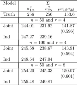
for correlations 0.6-0.9 in a two-level longitudinal model. These effects are the variance components from the second level. Average correlations are given in the parentheses. . . 37 Table A2.10 Average estimates of the variance components in the Σ design matrix
for errors in the two-level longitudinal model. Average correlations are given in the parentheses. . . 38 Table A2.11 Average estimates of the fixed effects and the standard errors from 100
simulations of a two-level longitudinal simulations with additional units / measurements. . . 39 Table A2.12 Average estimates of the components in the D design matrix for the
variance components at the top-level of a two-level longitudinal model with correlation ρ = 0.6 varying numbers of units / measurements. Average correlations are given in the parentheses. . . 40 Table A2.13 Average estimates of the variance components in the Σ design matrix
for errors in the two-level longitudinal model. Average correlations are given in the parentheses. . . 41
Table A4.1 This is the complete case situation forn= 1000 observations. . . 91 Table A4.2 This simulation corresponds to missing values in the response,y, the
structural response, Yi2, and discrete covariate. There was an average
of 9.8% missing rows. . . 92 Table A4.3 This simulation corresponds to missing values in the response,y, the
structural response,Yi2, and discrete covariate.There was an average of
Table A4.4 This simulation corresponds to missing values in the response,y, the structural response,Yi2, and continuous covariate. There was an average
missingness of 15.4% of the rows. . . 94 Table A4.5 This simulation corresponds to missing values in the response,y, the
structural response,Yi2, and continuous covariate. There was an average
of 43.5% missing rows. . . 95 Table A4.6 Results for the hierarchical structure with missing values in the response,y,
the structural response,Yi2, and discrete covariate. There was an
aver-age of 10.6% missing rows. . . 96 Table A4.7 Results for the hierarchical structure with missing values in the response,y,
the structural response,Yi2, and discrete covariate. There was an
aver-age of 43.6% missing rows. . . 97 Table A4.8 The estimated effect of Economic, Social, and Cultural Status (ESCS)
on mathematics performance. . . 99 Table A4.9 The estimated effect of Economic, Social, and Cultural Status (ESCS)
on reading performance. . . 100 Table A4.10 The estimated effect of Economic, Social, and Cultural Status (ESCS)
LIST OF FIGURES
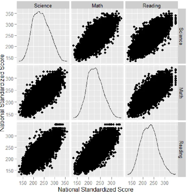
Figure A2.1 The scatterplot matrix of the science, mathematics, and reading test scores show that all three are highly correlated corroborating the use of a joint model. . . 42
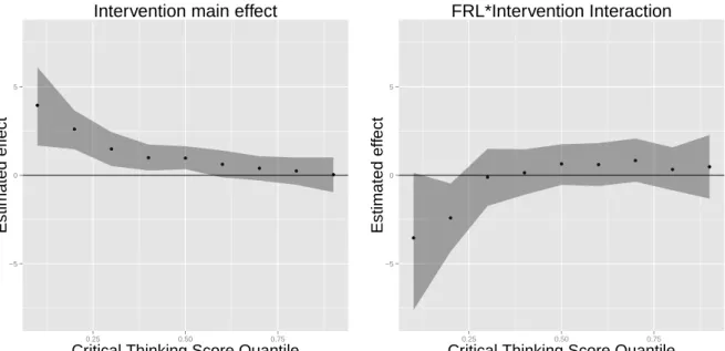
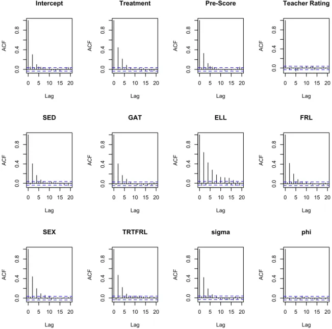
Figure A3.1 Plots of the estimated values for the treatment effect and the Free and Reduced Price Lunch/Treatment interaction effect for the 9 quantiles considered. The shaded area represents pointwise confidence intervals for each of the quantile estimates. . . 64 Figure A3.1 Locations of the 48 elementary schools in the study. . . 65 Figure A3.2 ACF plots of the autocorrelation from the MCMC for all of the fixed
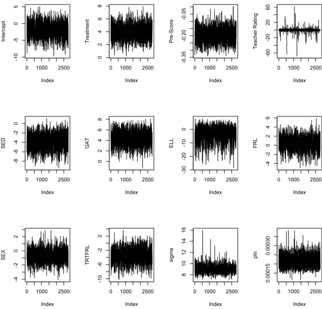
effects along with the two variances. . . 66 Figure A3.3 Plot of the mixing from the MCMC for all of the fixed effects along with
the two variances. . . 67 Figure A3.4 Plots of the estimates effects along with 95% credible intervals for each
of the parameters included in the model. . . 68 Figure A3.5 Plot of the cross quantile effects for special education students. . . 69 Figure A3.6 Mixing diagnostics for the τ1 = τ2 = 0.9 model for special education
students. . . 69 Figure A3.7 Density plots for theτ1 =τ2 = 0.9 model for special education students
based on the MCMC samples. . . 70
Figure A4.1 Scatterplots of the value for ESCS recorded for each student against students’ average plausible value in math, science, and reading for each student in the USA. . . 98
Figure A4.2 Estimated effect of ESCS on Mathematics for combinations of quantiles. The shaded area represents a 95% confidence region for the structural effect at each of the quantile combinations. . . 99 Figure A4.3 Estimated effect of ESCS on Reading for combinations of quantiles. The
shaded area represents a 95% confidence region for the structural effect at each of the quantile combinations. . . 100 Figure A4.4 Estimated effect of ESCS on Science for combinations of quantiles. The
shaded area represents a 95% confidence region for the structural effect at each of the quantile combinations. . . 101
ABSTRACT
This thesis focuses on many different modeling approaches that can be used to evaluate large education data sets. In education research, it is common to have multiple sources of variation designed into the study. If these are ignored, substantial bias can be introduced into the statistical model. We address this issue for three different classes of models: classical linear mixed effects models, quantile regression, and quantile regression of structural equation models. With the classical mixed effects model, we consider a joint modeling approach to estimation and evaluate the affect of correlation on the estimation of both fixed and random effects. For the structural equations models, we have evaluated the performance of a quantile regression impu-tation model. The other quantile regression model uses the Asymmetric Laplace Distribution to incorporate random effects with estimation performed using a bayesian approach.
Multivariate mixed effects models can be used to simultaneously model several outcomes. We look at the effect of different correlations on the model estimation. In our simulations, all of the off-diagonal correlations were the same. However, the estimation allowed the correlation matrix to be unstructured. We looked at both a longitudinal and hierarchical situation where predicted and parameters are selected to mimic situations seen in education research. The simulation results show that the joint modeling approach does not outperform a univariate modeling approach. The estimation of the covariances and correlations are unbiased when only random intercepts are included in the model. When random slopes are also included, the random effect variances tend to be underestimated using the joint modeling approach. Estimate of the correlations between similar random effects are good, but estimates of non-similar random effects exhibit severe bias.
Missing response and covariate values are common issues in large scale studies. We evaluate an imputation approach for quantile regression with recursive structural equations. In these models, the estimation of a structural effect is the primary concern. We apply an imputation
approach that uses quantile regression to impute missing values. We provide simulations eval-uating the estimation and 95% coverage from this approach both single-level and hierarchical data. Using this imputation approach for a recursive structural equation model, we provide an application studying the effect of selected quantiles of economic, social, and cultural status (ESCS) on selected quantiles for student test scores in mathematics, reading, and science from the PISA 2012 survey. Our findings show that when the rate of missingness is low (∼10%), the approach produces unbiased results with good coverage. When the rate of missingness is high (∼40%), the estimates show large bias and poor coverage. For the PISA 2012 application, the rate of missingness in the selected variables is low leading us to believe that the estimates are valid.
There is a dearth of quantile regression extensions to a mixed effects setting. In this paper we consider a bayesian approach using the asymmetric Laplace distribution (ALD). The loss function minimized in simple quantile regression is part of the kernel of the ALD. Further, the ALD can be represented as a mixture of normal and exponential distributions. Using this representation, conjugate prior distributions can be selected enabling straightforward gibbs sampling. Using the ALD, we model data from a large education study evaluating the impact of an intervention on critical thinking skills. We present two different models: a two-level model for all students and a two-level model for special education students. For the special education student model, we incorporate a quantile regression model for each level. This allows us to evaluate the impacts of the intervention in the tails of the student level and school level. For all the students, our results show that there is a significant impact from the intervention on the lower achieving students. For the special education students, the intervention is not significant, but the point estimates are mostly negative.
Keywords: Quantile Regression, Mixed effects modeling, multiple imputation, education data, structural equation model
CHAPTER 1. OVERVIEW
Linear Models have been almost synonymous with statistics for nearly 100 years. They have also been an integral part of much of the research conducted university-wide at Iowa State University since the creation of the Statistical Laboratory in the 1930s by George Snedecor. Despite the earliest account of linear regression dating back over 200 years to Legendre and Gauss in 1805 and 1809, linear models are ubiquitous in many disciplines and continue to be the subject of continuing research today. This is because, even in its simplest form, linear models provide a very flexible tool for researchers to evaluate the relationship between two or more variables. The knowledge gained from an increased understanding of the relationship among many different variables has had an immeasurable impact on scientific research.
As data collection methods became more refined, so did the models used to analyze the data. Linear Mixed Effects (LME) models are used to model individual-specific effects, cluster effects, and correlations among repeated measurements. A LME model identifies multiple sources of variation in the data as well as separating fixed individual effects from random group effects. A special case of the LME model is the multilevel model, where each level of data collection introduces a unique source of variation into the analysis. Further, the data values collected from the “clusters” at a higher level will be correlated. Typically there is a mixture of fixed effects predictors at each of the levels as well as random effect terms, which are incorporated to account for the variance from each of the levels of data collection.
For many years educational research has lacked a rigorous statistical approach. Conse-quently, there is very little consensus among educational researchers regarding educational effectiveness. In the last couple of decades there has been a concerted effort to improve the validity of the research through an emphasis on high-power randomized controlled studies. It is starting to be expected that researchers use appropriate statistical models that recognize model
assumptions, sources of variability, and possible biases from sources such as missing data and sample selection.
The vast majority of educational research that ventures past summary statistics involves regression-type models that focus on the mean. The idea of modeling the conditional mean is at the heart of many different regression approaches and has been an extremely useful tool for social science researchers. Under ideal conditions, these conditional-mean models have many attractive properties to social scientists, including ease of interpretability and ease of computation. They also have many attractive statistical properties and allow for modeling of the variance in cases of heteroscedasticity. In recent years, generalized linear models such as poisson regression for count data and logistic or probit regression for binary data have become increasingly popular.
While social scientists have been steadily using more sophisticated statistical models that more completely address the constraints and assumptions of their data, the limitations of conditional mean models still prevent them from directly addressing their primary research questions. It is common for researchers to be interested in the effect at non-central locations of the distribution. For instance, educational researchers typically are interested how an inter-vention affects the low achieving students (lower tail) and the high achieving students (upper tail). Using conditional mean models to address effects in the tails or specific portions of the distribution is simply a poor approach that is likely to be misleading.
This paper will address and examine a few of the multi-level scenarios that are common in educational research. A multivariate approach to modeling multiple outcomes simultaneously will also be examined as an improvement over univariate models. The efficacy of current ap-proaches used to evaluate level-2 effects will be evaluated and an alternative approach proposed to better understand effects at this level. Specifically, an evaluation is conducted of common models used to evaluate mediating variables for efficiency and error rates. A multi-level quan-tile regression approach to modeling level-2 effects is offered as an attractive alternative since it has the potential to describe a level-2 effect beyond the conditional mean.
1.1 Linear Models
The Linear Model is one of the simplest and most well known models in all of statistics. Its versatility leads to applications i in a broad range of disciplines. It attempts to model the mean of a measuredn×1 response vectorY conditioned on observed predictor variables. This leads to the following representation
Y =Xβ+ (1.1)
whereXis ann×pmatrix of predictor variables andis an×1 vector of random errors. In this simplest case, β represents a parameter vector of fixed effects. The usual assumptions in this model are independence and constance variance. Either least squares or maximum likelihood can be used to solve the normal equations to solve for the βparameter values. Either method leads to the solution
β= (XTX)−XTY
where (XTX)− is the generalized inverse in the case that (XTX) is not full rank.
1.1.1 Linear Mixed Effects Models
The Linear Mixed Effects (LME) model is a generalization of the linear model presented in Equation 1.1. Linear mixed effects models are used when there are correlated responses and the structure of the correlation can be specified in the variance matrix. The correlation arises when there are multiple sources of variability in then×1 response vectorY. These different sources of variability must be accounted for in the model. This leads to the following representation,
Y = Xβ+Zu+ (1.2)
u ∼ MVN(0,Ψ) ∼ MVN(0,Σ) (1.3)
whereX is ann×p matrix of predictor variables as in the simple linear model. Z is ann×q matrix of known constants, and β and u are p×1 andq×1 vectors of unknown parameters and random variables, respectively. It is very common to assume a constant variance for all the
identity matrix. When the joint distribution of (u,) is multivariate normal, the mixed effects model has the following properties:
E[Y|X, Z] = Xβ
Var[Y|X, Z] = Σ +ZΨZT.
In the case of a multilevel model, the Z matrix can be decomposed into pieces representing each of the additional variance components at each of the klevels in the design.
Y =Xβ+Z1u1+· · ·+Zkuk+ (1.4)
1.1.2 Multivariate Linear Mixed Effects Models
There are many scenarios when multiple responses from the same subject are recorded si-multaneously. In many cases it is likely that these these variables will be highly correlated. Searle et al. (1992) suggested an approach to simultaneously model multiple responses within the linear model framework. Linearizing the response vector and the design matrices allows for traditional computational approaches to be applied. Such modeling can lead to more efficient inference than separate univariate analyses. Shah et al. (1997) used this approach to simulta-neously model bivariate responses from two randomized trials evaluating a daily prophylactic treatment. This joint modeling approach determined the efficacy of the treatment and also es-timated the correlation between the CD4 and CD8 cell counts over time. Wu (2010) described the model and its estimation in the general form. Extensions of this approach incorporating measurement error and missing responses were considered by Liu and Wu (2007). This work was expanded upon later with a greater emphasis on modeling the missing data mechanism (Wu et al. (2009)).
We define the three subtest scores to be the p response variables. Subject i in the study will have ni repeated measurements of the p response variables. Let yijk be thekth response
value for studentiat timetij, and leteijkbe the corresponding random error,i= 1, . . . , n; j=
1, . . . , ni; k= 1, . . . , p. Let yik = (yi1k, . . . , yini,k)
T be the repeated measurements for student
Define eik and ei similarly. Let zil= (zi1l, . . . , zinil)
T be the covariate repeated measurements
of the l−th covariate of studenti,l= 1, . . . , p.
To incorporate the correlation between the different responses, we consider a multivariate version of the linear mixed effect model. LetΣbe thep×pcovariance matrix for thepresponse variables,
Cov(yiT1, . . . ,yipT) = Σ = (σij)p×p (1.5)
Let Xi and Zi be known design matrices that account for the structure of the repeated
mea-surements and the hierarchical nature of the data collection. LetXi = diag(Xi1, . . . ,Xip) be a
block diagonal matrix with thek−th block being matrixXikand letZi= diag(Zi1, . . . ,Zip) be
a block diagonal matrix with the k−th block being matrix Zik. Then we obtain the following
multivariate linear mixed effects model
yi =Xiβ+Ziγi+ei i= 1, . . . , n (1.6)
whereβ= (βT1, . . . ,βKT)T are fixed effects,γi = (γiT1, . . . ,γikT)T are random effects,bi∼N(0,D), γi ∼N(0,R), andei ∼N(0,Σ⊗Ii). D and R are unstructured covariance matrices that will
be estimated. The multivariate linear mixed effects model jointly models the different response variables incorporating the correlation among the responses through the covariance matrix Σ. It incorporates within subject and other sources of correlation through the random effects variance matrixD.
The most common approach to estimation is using the EM-algorithm. An assumption of joint normality of random effects, the residuals, and the response is generally made as is simplifies the expectations. Alternative estimation approaches were also addressed, such as Laplace approximations of the joint log-likelihood.
1.1.3 Contribution
Current and past research involving this joint modeling approach is limited. There is no research evaluating the influence of intraclass correlation on the estimation. This paper will evaluate, through simulation, how intraclass correlation in two and three level models affects the estimation of fixed effects. The estimates and corresponding standard errors will be compared
to estimates from a univariate model. These results will illustrate when it is beneficial to use a joint modeling approach rather than the simpler univariate approach. The asymptotic Fisher information is used to calculate standard errors.
1.2 Quantile Regression
Classical linear regression models the conditional mean providing a useful but incomplete summary of a collection of distributions. One of the earliest alternatives to conditional mean-based regression was median regression, which dates back to the 18th century. By modeling the response as a function of a specified conditional quantile rather than the conditional mean, quantile regression facilitates a complete analysis of the conditional distributional properties of the response variable. Similar to the linear regression framework, the quantile function is a linear function of the covariates taking the following form
Qyi(τ|xi) =xiβτ (1.7)
whereQyi(τ|xi) is the inverse cumulative distribution function ofygivexifor a givenτ ∈(0,1).
By specifying theτthconditional quantile function as a function of predictor variables we have the alternative minimization problem
min β∈Rp n X i=1 ρτ(yi−xtiβ). (1.8)
where ρτ(u) =u(τ −I(u < 0)). Solving for β(τ), which is a function of the selected quantile,
can be done very efficiently using linear programming methods.
Since the seminal work of Koenker and Bassett (1978), quantile regression methods have been extended well beyond the simple linear regression case. Everything from non-parametric smoothing techniques to penalized regression (such as Lasso) to ARMA models to multivariate quantiles to generalized quantile regression approaches to model binary and count data have been studied. However, there have been relatively few approaches developed for situations where there are multiple sources of variation. An overview of inferential and computation issues is covered extensively in Koenker (2005).
1.2.1 Modeling Longitudinal Data
Quantile regression has not easily extended to the linear mixed effects model because of the greater complexity in solving the minimization problem. Koenker (2005) considered using the penalized interpretation of the random effects estimation with a subject specific fixed effect to model longitudinal data. He considered estimators of the form
( ˆα(τ),βˆ(τ)) = arg min (α,β) X i X j ρτ(yij−xTijβ−αi) +λ n X i=1 |αi| (1.9)
By treating the subject-specific effect as fixed, this approach mitigates the distributional com-plications from additive random effects. This approach essentially reduces to a quantile function for each individual of the form
Qyij(τ|xij) =x
T
ijβ(τ) +αi(τ). (1.10)
This breaks the quantile function down into two component parts. There is a common popula-tion quantile funcpopula-tion plus an individual component for each subject. When the populapopula-tion are of interest, a penalty method that controls for the subject variability can be a useful approach due to the computational simplicity.
Reich et al. (2010) also considered adding a “subject”-specific effect for modeling clustered data, but from proposed a semi parametric Bayes approach. They considered modeling the residual distribution as an infinite mixture of simple densities that each satisfied a specific con-straint regarding the desired quantile. This approach incorporates correlation within subjects and outperformed traditional frequentist approaches when the true residual distribution was non-Laplacian.
More recently, many authors have been considering Bayesian hierarchical models with the Asymmetric Laplace Distribution (ALD). The mean parameter of the ALD is modeled as a combination of fixed and random effects. Usually, known conjugate prior distributions are chosen for the fixed and random effects parameters. Given n independent observations, this produces the following likelihood for the data
p(y|β) =τn(1−τ)nexp ( − n X i=1 ρτ(yi−µ) ) (1.11)
whereµis a location function. This method can be thought of as being similar to a generalized linear model where the link function isρτ(u). The ALD has gained popularity because it has
the property that it can be expressed as a scale mixture of a normal distributions (Tsionas (2003)). An asymmetric Laplace random variable can be represented as
Y =µ+ζW +σZpW/δ (1.12) whereζ = τ1(1−−2ττ) andσ = τ(12−τ). W and Z are mutually independent random variables where W is an exponential random variable with mean δ−1 and Z is a standard normal random variable. This leads to the following hierarchical structure
y|w∼N(µ+ζW, σ2δ−1W) and W ∼Exp(δ). (1.13)
In the quantile regression context,µ=xβ(τ). Yu and Moyeed (2001) showed that all posterior moments of β(τ) exist under a normal prior distribution. Kozumi and Kobayashi (2009) de-rived the conditional distributions assuming a standard exponential random variable,W, and showed that the resulting conditional distributions are proper. The conditional distribution for theβ(τ), conditioned onW andywas multivariate normal. The conditional distribution forW conditional on y and β(τ) was a generalized inverse Gaussian distribution. This greatly sim-plifies sampling from the posterior distribution because a Gibbs Sampler can be used. Kozumi and Kobayashi (2009) extend this result to the case containing the scale parameter and show that it again results in proper conditional distributions allowing a Gibbs Sampler to be used to sample from the posterior distribution.
Using this approach with ALD, Geraci and Bottai (2007) expanded the repertoire of subject-specific effect approaches using a hierarchical model. The linear mixed quantile function was modeled as
Qyij|ui(τ|xij, ui) =xij
Tβ+u
i i= 1, . . . , ni, j= 1, . . . , N (1.14)
where Qyij|ui(τ|xij, ui) is the cdf of the response conditional on a location-shift random effect
ui. Assume that yij observations, conditional on ui, are independently distributed and follow
an ALD. The mean parameter of the ALD is modeled as a linear function of predictors along with a subject-specific random effect, µ = xTijβ+ui. It is assumed that the ui are
parameters and that they are mutually independent of the residual errorsij. In this approach
it was proposed to model the ui using the ALD for a given τ. The degree of skewness (τu)
of the random effects distribution could also be estimated if the assumption of symmetry was unreasonable. Estimation was then accomplished using Gibbs Sampling.
This approach generalized very nicely to more complicated linear mixed effects model analogs. Rather than simply add a subject-specific effect, a vector of random effects and a structured design matrix can easily be incorporated into the mean of the ALD. Yuan and Yin (2010) considered this approach to model intermittent missingness and dropout in longitudinal data. They proposed using the followingl2−penalized check function to shrink the individual
effects and thereby borrow strength across subjects,
n X i=1 X j∈Ji,obs ρτ(yij−xTijβ−zijTb) + 1 2 n X i=1 bTiΛbi (1.15)
where Ji,obs denotes the set of all times when an observation was collected. bi is a vector
of unknown subject specific random effects and λis a nonsingular matrix. Λ acts as a tuning parameter to control the amount of shrinkage. The responses were modeled hierarchically using a normal prior for the random effects. The emphasis in this approach was to move beyond a single subject random effect and then incorporate these random effects into the missing data mechanisms.
Luo et al. (2012) used the ALD to incorporate a vector of random effects in a hierarchical bayesian approach. This is a fully parametric approach. Using the decomposition of the ALD into the scale mixture of normals, conjugate prior distributions are available allowing for Gibbs sampling without any complex sampling steps. This hierarchical approach assigned a normal prior distribution to the random effects. Yue and Rue (2011) considered an autoregressive case where random effects are necessary to account for overdispersion by either heterogeneity or correlation in longitudinal data. Gaussian Markov random fields priors with different forms and different degrees of smoothness were assigned to the covariates in conjunction with a continuous response.
1.2.2 Recursive Structural Equation Modeling
Ma and Koenker (2004) proposed a recursive structural equation modeling approach to address multiple sources of variability. This approach also had the benefit that the quantiles could vary across the equations. This approach is similar to the simultaneous equation model in econometrics
Y1 = Y2α+X1β+u1≡Zγ+u (1.16)
Y2 = Xδ+ν (1.17)
where X = [X1|X2]. It is assumed that u and ν are uncorrelated and that covariate X2 does
not show up in the equation for Y1. This simultaneous equation approach can be extended
beyond two equations. This simultaneous equations approach was used to estimate structural quantile treatment effects and two different classes of estimators were provided to estimate these effects. This approach was then used to evaluate the effect of class-size on student achievement allowing for inferences across all quantiles of both the distribution of class sizes and student achievement. Currently, extending quantile regression methods to data with multiple sources of variability is an active area of research.
1.2.3 Missing Data
Just as missing data can lead to misleading estimates in traditional regression analyses, it also has a big impact in quantile regression. Many of the traditional approaches to missing data have been directed at attempts to estimate a conditional mean. Mean-substitution, last-value forward, clustering imputation approaches, and even multiple imputation have imputed missing values that attempt to get unbiased estimates of a mean. Since quantile regression is modeling a conditional quantile, these imputation approaches will lead to biased estimates. There have been a couple attempts to extend multiple imputation to quantile regression by using a model of the conditional quantile for the imputation. Other approaches have used an ALD hierarchical model and incorporated models of the missingness.
Wei et al. (2012) proposed a multiple imputation estimator for quantile regression models. In the proposed approach at least one covariate must be completely observed and other
co-variates are assumed to be missing at random. Yuan and Yin (2010) considered this approach to model intermittent missingness and dropout in longitudinal data. They proposed using a l2−penalized check function to shrink the individual effects and thereby borrow strength across
subjects. Geraci (2013) evaluated another approach to applying multiple imputation methods to quantile regression for complex surveys when data was missing at random. Imputation of continuous variables was accomplished using the empirical distribution to preserve distribu-tional relationships in the data including skewness, kurtosis, and bounded outcomes. Chained equations were used to accomplish the sampling and the quantile regression model was speci-fied within the sampling process. Sherwood et al. (2012) studied a weighted quantile regression estimator in the presence of missing data. They showed that this estimator was consistent and asymptotically normal and illustrated the consistency through simulations. Further work addressing missing data within the quantile regression framework is needed.
1.3 The Future of Quantile Regression
With the increasing popularity of quantile regression, it seems realistic that the methodology will be extended to a wide variety of statistical applications. Koenker (2005) described this potential as the “Twilight Zone” and provided a few applications in areas where there are sure to be extensions and a significant presence. These areas included: multi-level models, binary and count data, survival analysis, and other important areas. In a presentation, Geraci (2011) supplemented the “Twilight Zone” with many models and applications needing further development that are of great importance to medical researchers. He listed missing data, spatial data (semi-parametric spline models), double-robust median regression (e.g. application to meta-analysis), and multilevel (>2) models as important areas for future development. His final remark specifically regarded the the need for model developments in longitudinal/hierarchical developments of quantile regression.
1.3.1 Contribution
A specific issue that has not been adequately addressed is the case when data are collected at multiple levels and inferences regarding each of those levels are of interest. The structural
equation approach of Ma and Koenker (2004) is limited in that it requires all the endogenous variables be continuous. It also requires the same sample size for each variable. In hierarchical situations, it could be misleading to manipulate the measurements from different levels into vectors of the same length. The approach that will be addressed here is an extension of the work from Luo et al. (2012) focusing on addressing inferences regarding data collected at a second level. The response will be modeling using an ALD with a meanµ=xTijβ+ui, where
ui is a level-2 specific effect. This level-2 specific effect will be modeled as ALD with a mean
as a function of measurements taken at that level plus the random effects. Combinations of quantiles at the two levels will be particularly informative for determining the effect of any covariate measured at level-2 contrasted with the response.
In addition to the common interest in making inferences at multiple levels of a data collec-tion design, the presence of missing data is a nearly ubiquitous issue in social science research. Wei et al. (2012) proposed amultiple imputation estimator for quantile regression models. In the proposed approach at least one covariate must be completely observed and other covariates are assumed to be missing at random. The approach was developed for models without random effects. Missing data approaches can be incorporated through the Bayesian approaches previ-ously mentioned using the prediction distributions as a step during the Markov Chain Monte Carlo sampling. Explicit missing data mechanism can also be formulated for when the data are not missing at random. We will explore different approaches to modeling missingness at multiple levels using the ALD framework.
CHAPTER 2. EFFECT OF CORRELATION ON THE ESTIMATION OF MULTIVARIATE MIXED EFFECTS MODELS
Abstract
Two issues that arise in many studies are multiple sources of variation and multiple response variables. Multivariate multiple regression allows for the responses to be simultaneously mod-eled. The effect of the correlation of the random effects on the estimation of both fixed effects and random effects is explored in this paper. Comparisons to a univariate approach are made to evaluate an improvements in estimation. A multivariate random effects model (Shah et al., 1997; Wu et al., 2009; Thum, 1997; Raudenbush et al., 1991) is selected to evaluate this effect on both longitudinal and hierarchical data. This paper evaluates the impact of correlation of random effects terms on the model estimation. An example using a cluster randomized trial is provided comparing both univariate and multiple modeling approaches along with a discussion of the benefit from each approach.
2.1 Introduction
There are many scenarios when multiple responses from the same subject are recorded simultaneously. In these cases, the relationship among the responses may be an important question. One approach to better understanding these associations is to use random-effects models and specifying the relationship in the distribution of the random effects. Searle et al. (1992) suggested an approach to simultaneously model multiple responses within the random-effects model framework (Laird and Ware, 1982). Linearizing the response vector and the design matrices allows for traditional computational approaches to be applied. This method, with extensions to handle missing data, has been considered in many different contexts. Due to the flexibility of random-effects models, the outcomes need not be similar. Comparisons of continuous, binary, integer, etc. data can be simultaneously modeled. It is not required that the same covariates be used to model each outcome nor the general model both be the same (e.g. linear and nonlinear models). Wu (2010) described the model and its estimation in the general form. Extensions of this approach incorporating measurement error and missing responses were considered by Liu and Wu (2007). This work was expanded upon later with a greater emphasis on modeling the missing data mechanism (Wu et al., 2009).
Using a data set measuring hearing threshold at two different frequencies, Fieuws and Verbeke (2004) evaluated the effect of a conditional independence assumption. Relaxing this assumption by allowing correlated errors resulted in the associations among the response vari-ables eliminated a source of bias in the estimation. Littell et al. (2000) used an example from the pharmaceutical industry to illustrate the effect on the fixed effects and variance compo-nents from different covariance structures. A method for selecting the best covariance structure, based on measures of model fit, was provided. Mikulich et al. (1999) explored the link between the multivariate and univariate mixed-effects approaches.
Modeling the effect of an intervention on more than one outcome is common in many different field including medicine and education. Shah et al. (1997) used this multivariate approach to simultaneously model bivariate responses from two randomized trials evaluating a daily prophylactic treatment. This joint modeling approach determined the efficacy of the
treatment and also estimated the correlation between the CD4 and CD8 – proteins found on the surface of immune cells – counts over time. Raudenbush et al. (1991) evaluated a survey measuring school climate based on five different dimensions. The stated motivation for using a multivariate, hierarchical mixed effects model was to simultaneously model the correlation among the five measures. Thum (1997) applied the multivariate approach to evaluate teacher engagement in school reform. The time spent on teaching activities along with the time spent on school governance activities were of interest. Both a univariate and multivariate model were considered in the analysis with the estimates nearly identical among common parameters.
This paper will evaluate the role of correlation in the estimation for the bivariate case. Two-level hierarchical and longitudinal cases are considered. Section 2.2 will describe the model and its estimation via an E-M algorithm (Dempster et al., 1977). Section 2.3 evaluate the different scenarios generated with various correlations. Section 2.4 summarizes the results of the simulations. Section 2.5 provides an example for a three response model evaluating the impact of a new approach teaching science in a cluster randomized trial. Section 2.6 provides a discussion of the simulations and the example providing conclusions.
2.2 Model
We follow the modeling approach and estimation for multivariate linear mixed effects model described by Shah et al. (1997). Suppose there are nindividuals with each individual having ni observations on m different response variables. Let yijk be the kth response for individual
i at time tij, and let eij be the corresponding random error, i = 1, . . . , n, j = 1, . . . , ni,
k = 1, . . . , m. The m response variables may be correlated. We define yij = (yij1, . . . , yijm)0
andYi = (yi01, . . . ,y0ini)
0, and definee
ij andEi similarly. We consider the following multivariate
linear mixed effects model
Yi1 .. . Yip = ˜ Xi1 .. . ˜ Xip β1 .. . βp + ˜ Zi1 .. . ˜ Zip b1 .. . bp + Ei1 .. . Eip (2.1) Yi=Xi∗β+Z ∗ ibi+Eij (2.2)
where Xij and Zij are design matrices containing covariates. We assume that the eij are
distributed i.i.d. N(0,Σ), the bi are distributed i.i.d. N(0,D), and the eij and the bi are
independent. The correlation among the responses is incorporated through the unrestricted covariance matrix Σ. We allow for arbitrary and non-ignorable missing data in the responses and covariates. Under the assumption of normality, the joint distribution of yi,bi, and ei is
multivariate normal as follows
yi bi ei ∼M V N Xi∗β 0 0 , Σ⊗Ii+Zi∗DZi∗T DZi∗T Σ⊗Ii Zi∗D D 0 Σ⊗Ii 0 Σ⊗Ii (2.3) Generally we have Xi∗= ˜ Xi1 .. . ˜ Xip = Xi1 · · · 0 .. . . .. ... 0 · · · Xip and Zi∗ = ˜ Zi1 .. . ˜ Zip = Zi1 · · · 0 .. . . .. ... 0 · · · Zip
are block diagonal matrices whereXik has dimensionsnik×qkandZikhas dimensionsnik×rk.
In the block diagonal structure Σ3k=1qk =q∗ and Σ3k=1rk =r∗.
Under these assumptions, the variances and covariances will generally take the form
var(b) =D = σβ2 1Ia · · · τβ1,βpIa .. . . .. ... τβ1,βpIa · · · σ 2 βpIa = σβ2 1 · · · τβ1,βp .. . . .. ... τβ1,βp · · · σ 2 βp ⊗Ia (2.4) and var(e) =R= σe21IN · · · τe1,epIN .. . . .. ... τe1,epIN · · · σ 2 e3IN = σe21 · · · τe1,ep .. . . .. ... τe1,ep · · · σ 2 ep ⊗IN (2.5)
Combining data vectors in such a way enables the use of standard estimation techniques such as Maximum Likelihood (ML) or Restricted Maximum Likelihood (REML) to be applied directly to the data.
2.2.1 Estimation via the Expectation-Maximization Algorithm
Estimation of the variance components and fixed effects is accomplished using the EM-algorithm (Dempster et al., 1977). Let τ index the iterations of the EM-algorithm τ = 1,2, . . . ,∞ where τ = 0 denotes the starting values. The sufficient statistics for Σ and D are P
(Ei0Ei) and P(b0ibi) respectively. Since bi and ei are unobservable the algorithm
com-putes the expectations of the sufficient statistics and then solves for the maximum likelihood. The joint density of yi,bi,ei is used to obtain the conditional expectations of the sufficient
statistics. Assuming normality the likelihood for the ith individual is
li =− 1 2Nlog(2π)− 1 2log|V −1 i | − 1 2(yi−X ∗ iβ)TVi−1(yi−Xi∗β) (2.6) whereVi=Σ⊗Ii+Zi∗DZi∗T
E-step: Let θ be the vector of the unknown parameters inΣand D and θ(τ) denote their
values after iteration τ. The estimate ofβ (Harville, 1977) given the current values of θ(τ) is
β(τ)= N X i=1 Xi∗0P(τ)Xi∗ ! N X i=1 Xi∗0P(τ)yi (2.7)
wherePi(τ) =Vi(τ)−1 and Vi =var(yi) = [Zi∗DZi∗0+ Σ⊗Ii]. Letting ri(τ) =yi−Xi∗β(τ) and B⊗2=BB0, the expectations for theith term of the sufficient statistics are given by
E[(bi)(bi)0|yi,θ(τ),β(τ)] ={E[bi|yi,θ(τ),β(τ)]}⊗2+V[bi|yi,θ(τ),β(τ)] (2.8)
E[(Eij)0(Eik)|yi,θ(τ),β(τ)] =E[Eij|yi,θ(τ),β(τ)]0E[Eik|yi,θ(τ),β(τ)] (2.9)
+tr[Cov(Eij,Eik|yi,θ(τ),β(τ)] j, k= 1, . . . , p
These expectations are easily obtained from the conditional mean and covariance matrix of the multivariate normal distribution.
M-step: In the M-step , Σ(τ+1) and D(τ+1) are found by equating them to the expected value of their sufficient statistics. For ML the iterative equations are
D(τ+1)= "N X i=1 h E[(bi)(bi)0|yi,θ(τ),β(τ)] i # /N (2.10) σjk = "N X i=1 ni #−1"N X i=1 h E[(Eij)0(Eik)|yi,θ(τ),β(τ)] i # j, k= 1, . . . , p (2.11)
whereσjkare the estimated individual components of var(e) at iterationτ as defined in equation
(2.5).
2.3 Simulations
Within education data many different multilevel data situations – longitudinal and hierar-chical – are common. This article applies joint estimation methods to the education context. In this section we will compare a simultaneous approach to an independent approach for both types of situations considering several two-level scenarios. The goal will be to evaluate the gains in efficiency from using a simultaneous modeling approach over a univariate approach. We will emulate a standardized testing scenario where the student is measured on at least two different tests. We consider different correlations between the random effects as well as different sample sizes.
2.3.1 Hierarchical Models
In the context of cluster randomized trials, the treatment is applied at the highest level. Within the two-level paradigm, we will consider both longitudinal and hierarchical situations that occur in educational research where the treatment is applied at the highest level. While it is not required that the covariates be the same for each model, in this simulation the models were generated using the same covariates with different values for the fixed effects. The values for the variances were selected to be similar to the observed values in the example data set examined in this article.
2.3.1.1 Two-Level
A two-level hierarchical model is considered for both outcomes. The covariates and pa-rameters were selected to closely mimic reasonable effects that may be seen when analyzing standardized test scores. The selection of variables includes: a linear grade level (G), a binary treatment variable (T), and two other binary covariates meant to mimic demographic indica-tor variables, (x3, x4). The binary variables are generated using a Bernouli random number
class level and all students in that class are exposed to the treatment. Equal numbers units are randomized to both treatment and control. Since each classroom is assumed to teach one grade, a random grade effect was not included. The model for both outcomes is as follows,
y1ij = β0+b0i+β1G1i+β2T1i+β3x3ij +β4x4ij +e1ij
y2ij = β5+b1i+β6G2i+β7T2i+β8x3ij +β9x4ij +e2ij (2.12)
wherei= 1, . . . , nare the classrooms andj = 1, . . . , sare the students in each classroom for a total of ns unique students providing 2ns test scores. The Gi and Ti are classroom level fixed
effect. Gi takes values 0,1,2,3 where each one unit increase emulates an increase of one grade
level. Each Ti represents the presence or absence of a treatment. x3 and x4 are simulated
binary variables at the student level emulating the present of various learning indicators. The random effects (b0i, b1i)0 ∼ MVN(0,D). The errors (e1ij, e2ij)0 ∼ MVN(0,Σ). The random
effects are independent of the errors. The covariance matrices take the form,
D= 20 20ρ 20ρ 20 Σ= 256 256ρ 256ρ 256
where correlations ofρ= (0.2,0.3,0.4,0.5,0.6,0.7,0.8,and 0.9) are considered. The covariances were selected to be similar to empirical covariances observed from univariate models. The parameter values for the fixed effects were set atβ = (150,15,4,7,2,150,15,4,4,6). Simulations were conducted for n= 50 and s= 15. The values for the fixed effect were selected based on estimates from the example data set in section 2.5. The sample size was selected to reduce computation time. A sample of 50 teachers with 15 students in each class seemed reasonably close to values that might be observed in a real study. To evaluate the gain from increasing the number of teachers or increasing the classroom size, additional simulations were conducted with the number of teachers doubled (n = 100) or the number of students doubled (s= 30). The correlation was fixed at 0.6 in the additional simulations.
2.3.2 Longitudinal Models
Since most interventions in education and other social sciences are not one-time events, but instead are a process that is administered over time, it is common for multiple measures to be
recorded throughout the duration of the study. Simulations in this article are conducted to evaluate the performance of the simultaneous estimation approach with two outcome variables. The covariates are the same for each model including covariates at the lowest and highest levels. Only a balanced design with the treatment assigned at the highest level is considered. The values for the variances were selected to be similar to the observed values in the example data set examined in this article.
2.3.2.1 Two-Level
A two-level longitudinal model includes only the repeated measures and the group experi-mental units as the two sources of variation. The treatment variable is a student-level variable that is time dependent. At time 0, all students are considered to be unexposed to the treatment. At all future times, half the students are assigned to the treatment group and half are assigned to the control group. Two time-independent covariates were created to emulate student demo-graphic covariates. There were again created using a Bernoulli distribution with probabilities 0.3 and 0.5 respectively. A random grade level effect is included to describe improvements due to time. These led to the following model for the two outcomes:
y1ij = β0+b0j+ (β1+b1j)G1ij +β2T1ij+β3x3ij+β4x4ij +eij
y2ij = β5+b2j+ (β6+b3j)G2ij +β7T2ij+β8x3ij+β9x4ij +eij (2.13)
where i= 1, . . . , n represents the nstudents each having j = 1, . . . , r repeated scores on each outcome. In the completely balanced case there are 2nrunique test scores. The random effects (b0i, b1i, b2i, b3i)0 ∼ MVN(0,D). The errors (e1ijk, e2ijk)0 ∼ MVN(0,Σ). The random effects
are independent of the errors. The covariance matrices take the form
D= 240 53.67ρ 244.95ρ 48.99ρ 53.67ρ 12 54.77ρ 10.95ρ 244.95ρ 54.77ρ 250 50ρ 48.99ρ 10.95ρ 50ρ 10 Σ= 256 256ρ 256ρ 256
where correlations ofρ= (0.2,0.3,0.4,0.5,0.6,0.7,0.8,and 0.9) are considered. The parameter values for the fixed effects were set at β = (150,15,4,7,2,150,15,4,4,6). Simulations were conducted with n= 50 and r = 4. Additional simulations we performed with the correlation fixed at 0.6 but with either the number of repeated measures doubled (r = 8) or the number of subjects doubled (n= 100). The values for the fixed effects were selected based to be similar to the values in the example in this article.
2.4 Results
In the simulations, the impact of both positively correlated random effects on model esti-mates for both hierarchical and longitudinal cases was evaluated. Changes to the sample sizes (at each level) were also considered to evaluate if there is any improvement in the estimates or additional benefit when using the joint modeling approach. In the hierarchal model, only a ran-dom intercept was considered while both ranran-dom intercepts and ranran-dom slopes were considered in the longitudinal case.
Tables A2.1 and A2.2 show the estimates of the fixed effects in the hierarchical case with n = 50 and s = 15. The estimates from both estimation approaches are nearly identical and very close to the true values. The standard errors are larger for effects at the top level (intercept: (β0, β5), grade:(β1, β6), and treatment: (β2 and β7)) and smaller for effects at the
lower level (x3: (β3,β8) and x4: (β4, β9)). This relationship holds for all correlations in both a
joint modeling approach and a univariate approach. If the estimates and the significance of the fixed effects is the primary concern then a univariate approach, available in standard software, would appear to be sufficient. The variance estimates in Table A2.3 show that the correlations among the intercepts are estimated very accurately. The estimates in theD matrix appear to be biased low. The estimates from the joint modeling approach are closer to the true value on average. None of the estimated D matrices degenerated to estimates of 0 which would have lowered the average from the 100 simulations. The estimates for the error matrix Σ are all very close to the true values. The correlation among the errors is unbiased and well estimated.
Increasing either the number of observational units (students) or the number of experimen-tal units (teachers) did not result in any advantage for the joint modeling approach. The results
are given in Table A2.4 and Table A2.5. With increases in the number of experimental units or observational units, the standard errors are identical until the 3rd decimal point for both the joint modeling approach and the univariate approach. As expected, increasing either the number of experimental units or observational units decreased the standard error of the esti-mates. Increasing the number of top level units had a greater impact on reducing the standard errors than increasing the number of lower level units. Increasing the sample sizes assuaged the bias in the estimates of the random effects. There was still a negative bias across all the random effects. Meanwhile, the estimates in the Σ error matrix were again very close to the true value. The estimates of the correlation in both theD and Σ matrices were very close to the true value of 0.6.
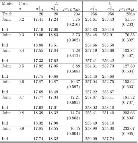
In the longitudinal case, both a random intercept and a random slope were considered. This allowed for each of the experimental units (students) to have their own slope. The results for varying correlations for the fixed effects can be seen in Tables A2.6 and A2.7. The standard errors using the joint modeling approach are smaller, at all correlations, for every fixed effect except the grade effects (β1andβ6). In this case all of the covariates are assigned at the student
level, but the treatment effect (β3 andβ7) is time dependent. All the fixed effects estimates are
close to the true values. There does not appear to be any systematic over- or under-estimating of any of the fixed effects. The estimates of the random effects can be seen in Tables A2.8 and A2.9. In every case the joint modeling approach is providing larger estimates of these random effects. The joint modeling approach produces larger estimates than the univariate approach for all the random effects. Both approaches ten to underestimate the intercepts and overestimate the slope. Both approaches do a poor job estimating the correlation between an intercept and a slope. The estimation of the correlation between two intercepts or two slopes is underestimated but much closer to the true values than the correlations between slopes and intercepts. With the joint approach consistently providing larger estimates of the random effect, the result is that the estimates of the error variance, seen in Table A2.10, are consistently smaller for the joint approach. Similarly, as the random effects showed a positive bias, the error variances show a negative bias. The estimation of the correlation between the two outcome performs well in the joint approach.
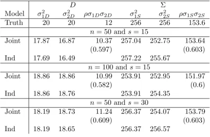
As expected, increasing either the sample size or the number of repeated measures resulted in smaller standard errors for each of the fixed effects. These can be seen in Table A2.11. Increasing the sample size resulted in a much bigger decrease on the standard errors of the fixed effects than increasing the number of repeated measures. The estimates for the both the Σ andD matrices with increased units/measurements can be seen in tables A2.12 and A2.13. Increasing the number of students did not seem to improve the estimation of the random effects or the error estimates. Both approaches still overestimate the random effects and underestimate the error variances. Increasing the number of repeated measures resulted in better estimation of the random slopes as well as improved estimation of the error variances. The estimates for the correlations were similar for the intercept-intercept and slope-slope correlation. However, the estimates of the correlation between the random slopes and intercepts was greatly improved with more measurements rather than more students. The correlation of the error variances for the two outcomes was estimated very well in every scenario.
2.5 Education Example
The SWH study involved a randomized cluster design of 48 elementary schools recruited for the study. The schools were randomly assigned into one of two equal-sized groups of 24 schools each. The treatment group was assigned to teach science using the SWH approach and the control group was assigned to continue teaching using the approach traditionally used by the individual school district. Five clusters were formed to control for differences in free and reduced lunch populations as well as concentrations of minority populations. The perfor-mances of schools and students were followed over the three-year duration of the study. In schools assigned to teach science using SWH, the approach was implemented in the 3rd, 4th, and 5th grades. Two schools that were recruited later into the project were randomized by placing one randomly in one group (i.e., control) and one in the second group (i.e., treatment). Due to the design of the study, there are many levels to the data structure. The interven-tion was applied at the school building level. Students are clustered within schools and over time. Consequently, there are three levels of variation that must be accounted for in any model.
Students were administered the Iowa Test of Basic Skills (ITBS) once a year. The test is subdivided into many smaller subject tests, including mathematics, science, and reading comprehension. The ITBS results for all students who had been enrolled at the schools recruited into the study between 2006 and the present were collected for analysis. The SWH intervention began during the 2010-11 academic year. Each year there were approximately 2,500 students in each grade among the 48 schools participating in the study. Starting in the 2011-12 academic year, the state of Iowa stopped using the ITBS and began using a new assessment instrument, the Iowa Assessments (IA); both sets of scores are provided by the Iowa Testing Program, at the University of Iowa. To account for this change we analyze the National Standardized scores for each subject test along with adding a fixed effect term for the test to account for changes in test difficulty.
Since the district had the option to determine when to administer the test, the timing of the ITBS/IA exams varied considerably within the year. As a result, exams are given as early as October and as late as April. A numeric variable identifying the trimester the exam was administered was constructed. To account for the development that occurs during this six-month period a term was added to the model to account for the different times the exam was taken.
All students are compared using the National Standardized Scores reported from the Iowa Testing Program, which equates the raw scores from the test into National Standardized Scores each year as one of the metrics to report back to schools and parents regarding student devel-opment. Table 1 shows that the mean and standard deviations are similar from year to year, with the exception of the 2011-12 year when the test changed from ITBS to IA and the mean decreased.
Of interest in the study was the overall effect of the SWH approach on science, mathematics, and Reading scores. Also of interest was the effect on different socioeconomic, demographic, and educational subgroups within the student population. To evaluate these effects we used a linear mixed effects model with random intercepts introduced for two separate levels (within student, among students). We estimate the same model for all three processes to facilitate comparison of the main effects and interactions. National standardized test scores from the
annual state performance exams in science, mathematics, and reading from 2006-2011 were used in model estimation.
2.5.1 Model and Results
The three tests – mathematics, science, and reading – are are jointly modeled over time. For a variety of reasons – all the tests were taken at the same time – it makes sense to model them simultaneously. Figure A2.1 corroborates this modeling choice as the three test processes appear highly correlated. The following models are selected for each test score
YScience=β0+b0+β1Grade + (β2+b1)TRT +β3FRL +β4GAT +β5IEP +β6ELL
+β7Semester +β8Test Form (2.14)
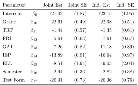
YReading=β9+b2+β10Grade + (β11+b3)TRT +β12FRL +β13GAT +β14IEP +β15ELL
+β16Semester +β17Test Form (2.15)
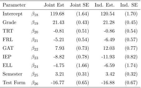
YM ath=β18+b4+β19Grade + (β20+b5)TRT +β21FRL +β22GAT +β23IEP +β24ELL
+β25Semester +β26Test Form (2.16)
where random effects for the intercept and treatment are also included into the model. The random effects for both the random effects bi and the errors ei are modeled as multivariate
normal with mean zero and unstructured covariance matrices. Estimates of all the model es-timates can be seen in Tables 2.1-2.3. These eses-timates are compared with eses-timates from a univariate linear mixed effects model. The covariance matrices for both the errors Σ and the random effects D, can be seen below. In both cases the covariances are on the top diagonal and the correlations are on the bottom diagonal.
Σ = 216.51 32.79 30.89 0.17 165.95 29.68 0.18 0.20 130.16 D= 326.67 52.21 328.94 42.38 244.40 31.15 0.84 11.68 54.48 8.60 49.62 9.48 0.95 0.83 366.66 59.32 241.70 40.29 0.58 0.62 0.77 16.12 36.92 11.56 0.86 0.92 0.80 0.58 246.32 44.77 0.45 0.72 0.55 0.75 0.75 14.46
The variances on the diagonals are very similar to the variances from univariate models of these processes. Comparisons of the joint approach to a univariate approach for all the variances can be seen in table 2.4. Comparisons of the fixed effects show that the estimates are very similar in both magnitude and direction, with few exceptions. The joint modeling approach leads to uniformly smaller standard errors.
Table 2.1 Science Scores
Parameter Joint Est Joint SE Ind. Est. Ind. SE Intercept β0 135.04 (2.03) 138.66 (2.14) Grade β1 18.96 (0.54) 18.39 (0.57) TRT β2 -1.44 (0.58) -0.79 (0.66) FRL β3 -6.61 (0.63) -8.56 (0.69) GAT β4 9.24 (0.85) 16.17 (0.96) IEP β5 -5.22 (0.91) -11.12 (0.99) ELL β6 -7.44 (1.94) -9.96 (2.08) Semester β7 3.18 (0.36) 3.00 (0.39) Test Form β8 -16.37 (0.82) -16.26 (0.86)
Table 2.2 Reading Scores
Parameter Joint Est Joint SE Ind. Est. Ind. SE Intercept β9 121.02 (1.87) 123.15 (1.95) Grade β10 22.61 (0.49) 22.38 (0.51) TRT β11 -1.44 (0.57) -1.35 (0.61) FRL β12 -5.61 (0.63) -7.61 (0.67) GAT β13 7.26 (0.82) 11.18 (0.89) IEP β14 -13.89 (0.91) -16.64 (0.97) ELL β15 -8.51 (1.94) -9.03 (2.04) Semester β16 2.94 (0.36) 2.82 (0.38) Test Form β17 -20.31 (0.73) -20.36 (0.76)
Table 2.3 Math Scores
Parameter Joint Est Joint SE Ind. Est. Ind. SE Intercept β18 119.68 (1.64) 120.54 (1.70) Grade β19 21.43 (0.43) 21.28 (0.45) TRT β20 -0.81 (0.51) -0.86 (0.54) FRL β21 -5.21 (0.54) -6.49 (0.57) GAT β22 7.93 (0.73) 12.03 (0.77) IEP β23 -8.82 (0.78) -11.93 (0.82) ELL β24 -4.75 (1.66) -6.59 (1.74) Semester β25 3.21 (0.31) 3.42 (0.32) Test Form β26 -16.77 (0.65) -16.88 (0.67)
Table 2.4 Comparison of variances between univariate and joint modeling
Term Univariate Model Joint Model Science Residual 224.65 216.51 Reading Residual 171.73 165.95 Math Residual 134.94 130.16 Science Intercept 292.13 326.67 Science Treatment 19.49 11.68 Reading Intercept 343.43 366.66 Reading Treatment 15.85 16.12 Math Intercept 227.91 246.32 Math Treatment 13.28 14.46
2.6 Discussion
In all the previous comparisons between the joint modeling approach and the univariate approach indicate that the benefits from a joint modeling approach is in the estimation of the correlations among different outcomes. The estimates of the fixed effect and their re-spective standard errors show that both approaches result in very similar estimates. In the case when there are only random intercepts, both of the approaches also perform similarly. When more random effects are included, there are other issues that arise. Both approaches tends to overestimate the random effects and underestimate the error variances. The over- and under-estimation of these effects is greater in the joint approach. In the hierarchical approach, increasing the number of top level units (teachers or schools) resulted in a greater benefit in both the estimation of the random effects and the error variances. In the longitudinal model, increasing the number of repeated measurements, resulted in better estimation of the random effects and error variances.
2.6.1 Contribution and Further Work
This article has evaluated the effect of correlation within a multivariate regression approach for modeling multiple outcomes simultaneously. While multiple outcomes are commonly corre-lated, there was no benefit to the estimation of the fixed effects due to the degree of correlation. The correlation also did not benefit the estimation of the variance components. The main ben-efit of this approach is to estimate correlations between random effects and errors for the multiple outcomes. Further work would be to evaluate more than two levels. The impact of model misspecification could also be evaluated.
2.7 Appendix
The appendix provides all the tables from both the longitudinal and hierarchical models as well as the figure from the example.
29 β0 β1 β2 β3 β4 β5 β6 β7 β8 β9 Model Corr. 150 15 4 4 6 150 15 4 4 6 Joint ρ= 0.2 149.57 15.09 4.20 3.76 6.15 150.49 14.94 3.66 3.90 5.95 (3.642) (0.755) (1.666) (1.297) (1.185) (3.639) (0.755) (1.663) (1.294) (1.183) Ind 149.56 15.09 4.20 3.76 6.16 150.49 14.94 3.66 3.90 5.95 (3.628) (0.752) (1.659) (1.297) (1.186) (3.637) (0.754) (1.661) (1.301) (1.189) Joint ρ= 0.3 150.22 14.94 3.95 4.00 6.06 150.19 14.93 4.04 4.07 6.07 (3.763) (0.775) (1.703) (1.296) (1.187) (3.755) (0.773) (1.699) (1.292) (1.183) Ind 150.22 14.94 3.95 4.00 6.06 150.19 14.93 4.04 4.07 6.07 (3.751) (0.772) (1.697) (1.297) (1.187) (3.746) (0.771) (1.694) (1.299) (1.189) Joint ρ= 0.4 150.25 14.95 3.90 4.04 6.06 150.22 14.93 4.07 4.08 6.11 (3.707) (0.761) (1.673) (1.304) (1.191) (3.710) (0.763) (1.675) (1.296) (1.184) Ind 150.26 14.95 3.90 4.04 6.05 150.22 14.93 4.07 4.08 6.11 (3.693) (0.758) (1.666) (1.305) (1.192) (3.709) (0.762) (1.673) (1.303) (1.190) Joint ρ= 0.5 149.97 14.97 4.00 4.08 6.10 149.63 15.05 3.99 4.04 6.12 (3.710) (0.771) (1.687) (1.295) (1.186) (3.659) (0.760) (1.663) (1.290) (1.181) Ind 149.97 14.97 4.00 4.09 6.09 149.63 15.05 3.99 4.04 6.12 (3.700) (0.769) (1.682) (1.295) (1.186) (3.649) (0.757) (1.658) (1.297) (1.188)
30 β0 β1 β2 β3 β4 β5 β6 β7 β8 β9 Model Corr. 150 15 4 4 6 150 15 4 4 6 Joint ρ= 0.6 150.65 14.88 3.86 3.99 5.81 150.75 14.86 3.96 3.82 5.86 (3.685) (0.756) (1.677) (1.302) (1.192) (3.618) (0.743) (1.646) (1.291) (1.182) Ind 150.65 14.88 3.86 3.99 5.81 150.75 14.86 3.96 3.82 5.86 (3.672) (0.754) (1.671) (1.303) (1.193) (3.606) (0.740) (1.640) (1.298) (1.188) Joint ρ= 0.7 149.56 15.08 4.18 4.18 5.90 149.45 15.09 4.25 4.00 5.93 (3.717) (0.763) (1.684) (1.304) (1.194) (3.678) (0.754) (1.667) (1.297) (1.187) Ind 149.56 15.08 4.18 4.18 5.90 149.45 15.09 4.25 4.00 5.93 (3.708) (0.761) (1.679) (1.305) (1.194) (3.670) (0.752) (1.662) (1.304) (1.194) Joint ρ= 0.8 150.03 15.00 3.88 3.81 6.21 149.95 15.02 3.88 3.87 6.16 (3.697) (0.766) (1.692) (1.295) (1.188) (3.682) (0.763) (1.685) (1.285) (1.179) Ind 150.03 15.00 3.88 3.81 6.21 149.95 15.02 3.88 3.87 6.16 (3.693) (0.765) (1.690) (1.296) (1.189) (3.673) (0.760) (1.680) (1.292) (1.185) Joint ρ= 0.9 149.68 15.05 4.04 4.07 6.02 149.86 15.02 3.98 4.11 5.94 (3.774) (0.775) (1.692) (1.306) (1.196) (3.794) (0.780) (1.702) (1.296) (1.188) Ind 149.68 15.05 4.04 4.06 6.02 149.86 15.02 3.98 4.10 5.94 (3.767) (0.773) (1.688) (1.306) (1.197) (3.791) (0.779) (1.700) (1.303) (1.194)