UCLA
UCLA Electronic Theses and Dissertations
TitleNeural network based representation learning and modeling for speech and speaker recognition Permalink https://escholarship.org/uc/item/6mm160gq Author Guo, Jinxi Publication Date 2019 Peer reviewed|Thesis/dissertation
UNIVERSITY OF CALIFORNIA Los Angeles
Neural network based representation learning and modeling for speech and speaker recognition
A dissertation submitted in partial satisfaction of the requirements for the degree
Doctor of Philosophy in Electrical and Computer Engineering
by
Jinxi Guo
c
Copyright by Jinxi Guo
ABSTRACT OF THE DISSERTATION
Neural network based representation learning and modeling for speech and speaker recognition
by
Jinxi Guo
Doctor of Philosophy in Electrical and Computer Engineering University of California, Los Angeles, 2019
Professor Abeer A. H. Alwan, Chair
Deep learning and neural network research has grown significantly in the fields of automatic speech recognition (ASR) and speaker recognition. Compared to traditional methods, deep learning-based approaches are more powerful in learning representation from data and build-ing complex models. In this dissertation, we focus on representation learnbuild-ing and modelbuild-ing using neural network-based approaches for speech and speaker recognition.
In the first part of the dissertation, we present two novel neural network-based methods to learn speaker-specific and phoneme-invariant features for short-utterance speaker verifi-cation. We first propose to learn a spectral feature mapping from each speech signal to the corresponding subglottal acoustic signal which has less phoneme variation, using deep neural networks (DNNs). The estimated subglottal features show better speaker-separation abil-ity and provide complementary information when combined with traditional speech features on speaker verification tasks. Additional, we propose another DNN-based mapping model, which maps the speaker representation extracted from short utterances to the speaker rep-resentation extracted from long utterances of the same speaker. Two non-linear regression models using an autoencoder are proposed to learn this mapping, and they both improve speaker verification performance significantly.
In the second part of the dissertation, we design several new neural network models which take raw speech features (either complex Discrete Fourier Transform (DFT) features or raw
waveforms) as input, and perform the feature extraction and phone classification jointly. We first propose a unified deep Highway (HW) network with a time-delayed bottleneck layer (TDB), in the middle, for feature extraction. The TDB-HW networks with complex DFT features as input provide significantly lower error rates compared with hand-designed spec-trum features on large-scale keyword spotting tasks. Next, we present a 1-D Convolutional Neural Network (CNN) model, which takes raw waveforms as input and uses convolutional layers to do hierarchical feature extraction. The proposed 1-D CNN model outperforms standard systems with hand-designed features. In order to further reduce the redundancy of the 1-D CNN model, we propose a filter sampling and combination (FSC) technique, which can reduce the model size by 70% and still improve the performance on ASR tasks.
In the third part of dissertation, we propose two novel neural-network models for sequence modeling. We first propose an attention mechanism for acoustic sequence modeling. The attention mechanism can automatically predict the importance of each time step and select the most important information from sequences. Secondly, we present a sequence-to-sequence based spelling correction model for end-to-end ASR. The proposed correction model can effectively correct errors made by the ASR systems.
The dissertation of Jinxi Guo is approved.
Alan J. Laub Yingnian Wu
Christina Panagio Fragouli Abeer A. H. Alwan, Committee Chair
University of California, Los Angeles 2019
TABLE OF CONTENTS
1 Introduction . . . 1
1.1 Overview and motivation . . . 1
1.2 Deep neural networks . . . 2
1.2.1 DNN architecture and optimization methods . . . 2
1.2.2 Convolutional Neural Networks . . . 4
1.2.3 Recurrent Neural Networks . . . 4
1.3 Speech processing and feature extraction . . . 6
1.4 Speaker Verification . . . 6
1.4.1 I-vector/PLDA system . . . 6
1.4.2 Speech corpora . . . 9
1.4.3 Evaluation metrics . . . 10
1.5 Automatic Speech Recognition . . . 11
1.5.1 DNN-HMM based speech recognition system . . . 11
1.5.2 End-to-end speech recognition system . . . 15
1.5.3 Speech corpora . . . 17
1.5.4 Evaluation metrics . . . 18
1.6 Dissertation Outline . . . 18
2 Learning speaker representations from short utterances . . . 19
2.1 Introduction . . . 19
2.2 Related work . . . 20
2.3 Learning speaker-specific and phoneme-invariant subglottal acoustic features 20 2.3.1 Subglottal acoustic features . . . 20
2.3.2 Proposed estimation method . . . 21
2.3.3 Estimation experiments . . . 22
2.3.4 Speaker verification experiments . . . 25
2.4 Learning non-linear mapping from short-utterance to long-utterance i-vectors 28 2.4.1 The effect of utterance durations on i-vectors . . . 28
2.4.2 DNN-based i-vector mapping . . . 29
2.4.3 Experimental set-up . . . 35
2.4.4 Evaluation of proposed i-vector mapping methods . . . 38
2.4.5 Speaker verification experiments . . . 40
2.5 Conclusion . . . 50
3 Joint feature learning and acoustic modeling for automatic speech recog-nition . . . 51
3.1 Introduction . . . 51
3.2 Related work . . . 51
3.3 Feature learning in the frequency domain . . . 52
3.3.1 Baseline Wake-word Detection System . . . 52
3.3.2 DFT-Input Highway networks . . . 54
3.3.3 Experiments and results . . . 57
3.4 Feature learning from raw waveforms . . . 62
3.4.1 CNN-based acoustic modeling using raw waveforms . . . 62
3.4.2 Filters learned from raw waveforms . . . 63
3.4.3 Filter sampling and combination CNN . . . 65
3.4.4 Experiments and results . . . 67
4 Sequence modeling for acoustic and language models . . . 73
4.1 Introduction . . . 73
4.2 Related work . . . 74
4.3 Learning attention mechanism for acoustic modeling . . . 74
4.3.1 Acoustic scene classification . . . 74
4.3.2 Neural network architectures . . . 75
4.3.3 Attention mechanisms for sequence modeling . . . 76
4.3.4 Evaluation set-up . . . 79
4.3.5 Experimental results . . . 80
4.3.6 Analysis of learned attention weights . . . 84
4.4 Learning a spelling correction model for end-to-end speech recognition . . . . 85
4.4.1 Motivation . . . 85
4.4.2 Baseline LAS model . . . 86
4.4.3 Approaches of utilizing text-only data . . . 87
4.4.4 Spelling correction model . . . 87
4.4.5 Experimental setup . . . 90
4.4.6 Experimental results . . . 93
4.4.7 Error analysis . . . 96
4.5 Conclusion . . . 97
5 Summary and future work . . . 99
5.1 Summary . . . 99
5.2 Future work . . . 101
LIST OF FIGURES
1.1 An LSTM block. At time step t, Ct and Ct−1 represent the current and
previ-ous cell states, ht and ht−1 represent the current and previous hidden states, ft
represents forget gate, it represents input gate, and ot represents output gate. . . 5
1.2 A standard ASR system. . . 11 1.3 Components of the LAS model. . . 16
2.1 Spectrograms of three vowels by a female speaker to compare within-speaker variability of microphone speech (top panel) and subglottal acoustics (bottom panel). Note that the subglottal acoustics don’t vary much. Data are sampled from the recordings of a female speaker in the WashU-UCLA corpus. . . 21 2.2 Histogram of the correlation coefficient of the actual and estimated subglottal
Mel-filterbank coefficients for each frame in the validation dataset. . . 23 2.3 Block diagram of the proposed framework. . . 26 2.4 Distribution of active speech length of 40000 long utterances in SRE and SWB
datasets. . . 29 2.5 DN N1: two-stage training of i-vector mapping. Left schema corresponds to the
first-stage pre-training. A short-utterance i-vector ws and a corresponding
long-utterance i-vector wl are first concatenated into z. Thenz is fed into an encoder
f(.) to generate the joint embeddingh. his passed to the decoderg(.) to generate the reconstructed ˆz, which is expected to be a concatenation of a reconstructed
ˆ
ws and ˆwl. Right schema corresponds to the second-stage fine-tuning. The
pre-trained weights in the first stage is used to initialize the supervised regression model fromwstowl. After training, the estimated i-vector ˆwlis used for evaluation. 31
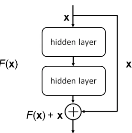
2.6 Residual block. An input xis first passed into two hidden layers to get F(x) and it also goes through a short-cut connection, which skips the hidden layers. The final output of the residual block is a summation of F(x) and x. . . 32
2.7 DN N2: single-stage training of i-vector mapping. A short-utterance i-vector ws
is passed to an encoder and the output of the encoder is first used to generate the estimated long-utterance i-vector ˆwl and it is also fed into a decoder to generate
the reconstructed short-utterance i-vector ˆws. The two tasks are optimized jointly. 32
2.8 I-vector mapping with additional phoneme information. A short-utterance i-vector ws is concatenated with a phoneme vector p to generate the estimated
long-utterance i-vectors ˆwl. . . 34
2.9 EER as a function of reconstruction loss α for DN N2. . . 44
2.10 DET curves for the mapping results of I-vector GMM and I-vector DNN systems under 10 s-10 s conditions of NIST SRE10 database. Left figure corresponds to female speakers and right one corresponds to male speakers. . . 48
2.11 Distribution of active speech length of truncated short utterances in the SITW database. . . 49
3.1 HMM-based Keyword Spotting. . . 53
3.2 Baseline WW DNN with the LFBE feature. . . 54
3.3 Whole WW Highway DNN with the DFT input. . . 56
3.4 DET curves of LFBE DNN, LFBE HW, DFT TDB-DNN, DFT TDB-HW using different amounts of training data . . . 59
3.5 AUCs calculated from Figure 3.4. . . 59
3.6 DET curves of LFBE HW, DFT TDB-HW, Audio TDB-HW, LPS TDB-HW using different amounts of training data . . . 61
3.7 AUCs calculated from Figure 3.6 . . . 61
3.8 Filters learned from each conv layer (order from top to bottom). Each row rep-resents a layer and 6 different filters from that layer are shown. . . 64
3.9 Widthwise filter sampling in space Φ. . . 65
4.1 The CLDNN framework . . . 76 4.2 Standard BLSTM layer (left), attention-based BLSTM layer (right) . . . 77 4.3 The mel-filterbank features (bottom) with time-aligned attention scores (top) for
the sample segment recorded in a cafe/restaurant . . . 83 4.4 The mel-filterbank features (bottom) with time-aligned attention scores (top) for
the sample segment recorded in a park . . . 83 4.5 Spelling Correction model architecture. . . 89 4.6 Example attention weights from the SC model. . . 94
LIST OF TABLES
2.1 J-ratio, a measure of class separation for different feature values. Features were extracted from isolated vowel recordings of speech and subglottal acoustics, for all the 50 male and female adult speakers in the WashU-UCLA corpus. . . 24 2.2 EERs for the MFCC baseline system and the fused system on the NIST SRE 08
truncated 10sec-10sec and 5sec-5sec evaluation tasks. The relative improvements in EERs are also shown. . . 27 2.3 Mean variance of long and short utterances (from the SRE and Switchboard
datasets) . . . 29 2.4 Datasets used for developing I-vector GMM and I-vector DNN systems . . . 35 2.5 Square Euclidean distance (Dsl) between short and long utterance i-vector pairs
from SRE10 before and after mapping. . . 39 2.6 J-ratio for short-utterance i-vectors from SRE10 before and after mapping. . . . 39 2.7 Baseline results for I-vector GMM and I-vector DNN systems under full-length
and short-length utterances conditions reported in terms of EER, Relative Im-provement (Rel Imp), and minDCF on NIST SRE10 database. . . 41 2.8 Results for baseline (I-vector DNN), matched-length PLDA training, LDA
di-mension reduction, DNN direct mapping and proposed DNN mapping in the 10 s-10 s condition of NIST SRE10 database. . . 42 2.9 DNN-based mapping results using DNNs with different depths in the 10 s-10 s
condition of NIST SRE10 database. . . 45 2.10 DNN-based mapping results with additional phoneme information in the 10 s-10
s condition of NIST SRE10 database. . . 46 2.11 DNN-based mapping results with different utterance durations on NIST SRE10
2.12 Results for I-vector GMM and I-vector DNN systems in the 10 s-10 s conditions of NIST SRE10 database. . . 48 2.13 DNN-based mapping results on SITW using arbitrary durations of short utterances. 49
3.1 Proposed 1-D CNN structure (the last column shows the number of parameters for each layer). . . 63 3.2 Baseline comparison: different features and neural network structures. . . 69 3.3 Filter sampling results for raw waveform CNNs. ‘c∗’ indicates that the
convo-lutional layers have half the number of filters in each layer compared with the baseline CNN. ‘cw’ and ‘cd’ represent compressing the parameters in the con-volution layers using widthwise and depthwise filter sampling, respectively. ‘fw’ represents performing widthwise filter sampling in the fully connected layers. ‘/4’ means reducing the number of parameters by a factor of 4. . . 70 3.4 Filter sampling and combination results for raw waveform CNNs. lin-MxN means
doing linear combination using MxN different scalars. . . 71
4.1 Classification accuracy (%) of CNNs and CLDNNs . . . 80 4.2 Classification accuracy (%) of CBLDNNs and different attention models . . . . 81 4.3 Classification accuracy (%) of CBLDNNs, attention model and 3 combined models 82 4.4 Word error rates (WERs) on LibriSpeech “clean” sets comparing different
tech-niques for incorporating text-only training data. Numbers in parentheses indicate the number of input hypotheses considered by the corresponding model. . . 93 4.5 Oracle WER before and after applying the SC model. . . 95 4.6 Word error rates (WERs) on LibriSpeech “clean” sets comparing different
tech-niques for incorporating text-only training data. Numbers in parentheses indicate the number of input hypotheses considered by the corresponding model. . . 95 4.7 WER comparison on a real audio and TTS dev sets. . . 96
4.8 Word error rates (WERs) on LibriSpeech “clean” sets comparing different tech-niques for incorporating text-only training data. Numbers in parentheses indicate the number of input hypotheses considered by the corresponding model. . . 96 4.9 LAS + SC + LM rescore Wins. LAS + LM rescore (in bold) . . . 97
ACKNOWLEDGMENTS
This dissertation would not have been possible without the support of many people. I would like to first thank my advisor Prof. Abeer Alwan, for being a great mentor over the years and providing me with gracious support. Her vision for speech processing motivated me to start my PhD research. She has given me great freedom to pursue the research that I would like to work on. I am also indebted to Prof. Yingnian Wu for his insightful suggestions to my research. I would like to also thank the rest of my committee member, Prof. Alan Laub and Prof. Christina Fragouli, for their invaluable advice and comments on my dissertation. I am also grateful to have worked with Dr. Ning Xu at Snap. Ning’s sound knowledge and nice personality made my internship and our further collaborations a great pleasure for me. Many thanks to Dr. Kenichi Kumatani, I have enjoyed and benefited a lot from various discussions with him during the internship at Amazon Alexa team. Sincere appreciation also goes to Dr. Tara Sainath and Dr. Ron Weiss for their supervision during my summer internship at Google. Their mentorship has immensely impacted my thought process both as a person and as a researcher.
My heartfelt thanks also go to my former and current labmates at SPAPL. Many thanks to Jom, Gang, Harish, Lee, and Anirudh for helping me find my bearings initially. Without their help, I would not have been able to start my life and work easily at UCLA. I am also grateful to Soo, Amber, Gary, Vijay, Kaan, Rohit, Ruochen, Hitesh and Angli for many enjoyable discussions and collaborations. Many thanks to Kailun, Yang, Kaiyuan, Usha, Deepak for the collaborations directly related to this dissertation. My work would not have been possible without their support.
I also extend my gratitude to the administrative staff in the department (especially Deeona and Ryo) for their patience and tremendous help throughout my entire PhD period. Life would have been a lot tougher without them. I am truly blessed with my wonderful friends in Swipe group. I am thankful for their company, support and many enjoyable chats.
Lastly, but very importantly, a million thanks to my family members for their uncondi-tional love and enormous support. My father Hongfu Guo and my mother Shumei Du have made a lot of sacrifices to ensure that I could focus on my research and career goals. A big thank you to Xiaoxi for her love, understanding and company.
VITA
2009-2013 B.E., Electronics and Information Engineering, Xi’an Jiaotong University, China.
2013-2015 M.S., Electrical Engineering, University of California, Los Angeles, USA.
2013–2019 Graduate Research Assistant, Electrical and Computer Engineering De-partment, UCLA.
2014–2017 Teaching Assistant, Electrical and Computer Engineering Department, UCLA.
2015 Research Internship, Qualcomm.
2016 Research Internship, Snap Inc.
2017 Research Internship, Amazon.
2018 Research Internship, Google.
PUBLICATIONS
Jinxi Guo, Tara Sainath and Ron Weiss, “A spelling correction model for end-to-end speech recognition,” ICASSP, 2019.
Jinxi Guo, Ning Xu, Kailun Qian, Yang Shi, Kaiyuan Qian, Yingnian Wu and Abeer Alwan, “Deep Neural Network based i-Vector mapping for Speaker Verification using Short Utterances,” Speech Communication, 2018.
Jinxi Guo, Ning Xu, Xin Chen, Yang Shi, Kaiyuan Qian, Yingnian Wu and Abeer Al-wan, “Filter sampling and combination CNN (FSC-CNN): a compact CNN model for small-footprint ASR acoustic modeling using raw waveforms,” Interspeech, 2018.
Jinxi Guo, Kenichi Kumatani, Ming Sun, Minhua Wu, Anirudh Raju, Nikko Strom and Arindam Mandal, “Time-delayed bottleneck Highway Networks using a DFT feature for Robust Keyword Spotting,” ICASSP, 2018.
Jinxi Guo, Ruochen Yang, Harish Arsikere and Abeer Alwan, “Robust speaker identifica-tion via fusion of Subglottal Resonances and Cepstral Features,” Journal of Acoustic Society of American, 2017.
Jinxi Guo, Usha Nookala and Abeer Alwan, “CNN-based joint mapping of short and long utterance i-vectors for speaker verification using short utterances,” Interspeech, 2017.
Jinxi Guo, Ning Xu, Li-Jia Li and Abeer Alwan, “Attention based CLDNNs for short-duration acoustic scene classification,” Interspeech, 2017.
Jinxi Guo, Gary Yeung, Deepak Muralidharan, Harish Arsikere, Amber Afshan and Abeer Alwan, “Speaker verification using short utterances with DNN-based estimation of subglottal acoustic features,” Interspeech, 2016.
Jinxi Guo, Rohit Paturi, Gary Yeung, Steven M Lulich, Harish Arsikere and Abeer Alwan, “Age-dependent height estimation and speaker normalization for children’s speech using the first three subglottal resonances,” Interspeech, 2015.
Jinxi Guo, Angli Liu, Harish Arsikere, Abeer Alwan and Steven M Lulich, “The relationship between the second subglottal resonance and vowel class, standing height, trunk length, and F0 variation for Mandarin speakers,” Interspeech, 2014.
CHAPTER 1
Introduction
1.1
Overview and motivation
Automatic Speech Recognition (ASR) and Speaker Recognition (SV) are two very important applications. There have been extensive studies conducted of both tasks over the past decade. However, there are still challenging problems.
For SV, state-of-the-art text-independent systems exhibit satisfactory performance with adequately long speech data (e.g. more than 30 s), but the performance degrades rapidly when only limited data are available [KVD11]. The degraded performance is due to the large phonetic (context) variation between different short utterances. The requirement of significant amounts of speech for training or evaluation, especially with large intersession variability has limited the potential of SV’s widespread implementations in practice. To address this issue, a range of techniques has been studied on different aspects of this problem [PSS17, DP18]. However, learning a speaker-specific and phoneme-invariant representation from short utterances is still very challenging.
For ASR, constructing an appropriate feature representation and designing an appropri-ate phone classifier for these features have often been treappropri-ated as separappropri-ate problems in the speech recognition community. One drawback of this approach is that the designed features might not be best for the classification objective at hand. In order to solve this problem, Deep Neural Networks (DNNs), and their variants, can be used to perform feature extrac-tion jointly with classificaextrac-tion. However, for a long time, the most popular features to train DNNs remain the log-mel features. The mel filter bank is inspired by auditory evidence of how humans perceive speech signals. Such a filter bank may not always be the best filter
bank in a statistical modeling framework where the end goal is word error rate. To address this issue, there have been various attempts [BR15, HWW15, SWS15] to use a simpler fea-ture representation (e.g. waveforms) with neural networks to learn feafea-ture representation jointly with the rest of the network. However, only a few studies have shown improvement over the log-mel trained model.
Moreover, sequence modeling is one of the key problems for speech modeling. Traditional systems use Hidden Markov Models (HMMs) to model speech sequences. In recent years, Recurrent Neural Networks (RNNs), and their variants (e.g. Long Short Term Memory (LSTM) networks), have shown superior performance on various speech sequence modeling tasks compared with HMMs. However, the basic RNN models still need to be modified in order to perform modeling on advanced tasks, such as information selection and sequence-to-sequence modeling (e.g. end-to-end ASR).
In this dissertation, in order to address the aforementioned problems and challenges in ASR and SV, several DNN based approaches are proposed and discussed. Compared to tradi-tional methods, deep learning-based approaches are more powerful in learning representation from data and building complex models. Therefore, we present novel neural network-based approaches to perform representation learning and modeling.
In this chapter, we will review some background knowledge for deep neural networks, speech processing, speaker verification and automatic speech recognition systems.
1.2
Deep neural networks
1.2.1 DNN architecture and optimization methods
A deep neural netowrk (DNN) is a conventional multilayer perceptron (MLP) with many (often more than two) hidden layers. In all L−1 hidden layers:
wherevl,Wl,blare the activation vector, the weight matrix and the bias vector, respectively
at layer l. Wl is a N
l×Nl−1 matrix, where Nl represents the number of neurons at layer l.
In many applications, the sigmoid function, the hyperbolic tangent function or the rectified linear unit (ReLU) function is used as the activation function.
The output layerLneeds to be chosen based on the tasks in hand [YD16]. For a regression task, a linear layer is typically used to generate the output vector vL with dimension NL:
vL =WLvL−1+bL (1.2)
For multi-class classification tasks, each output neuron represents a class i∈ {1, ..., C}, where C = NL is the number of classes. The value of the ith output neuron vLi represents
the probability Pdnn(i|o) that the observation vector o belongs to class i. To be a valid
multinomial probability distribution, the output vector vL should satisfy the requirements
thatviL>0 andPC i=1v
L
i = 1. This can be done by normalizing the excitation with a softmax
function: vLi =Pdnn(i|o) = softmaxi(zL) = ezL i PC j=1e zL j (1.3)
The model parameters {W,b} in a DNN are unknown and need to be estimated from training samples for each task. In order to perform parameter estimation, a training criterion and a learning algorithm need be specified.
The training criterion should be highly correlated to the final goal of the task. There are two popular empirical training criteria in DNN model learning. For regression task, the mean square error (MSE) criterion is typically used:
JM SE(W,b;o,y) =
1 2(v
L−y)T(vL−y) (1.4)
where {W,b} are the model parameters, o is the observation, and y is the corresponding output vector.
For classification tasks,yis a probability distribution and the cross-entropy (CE) criterion is often used: JCE(W,b;o,y) =− C X i=1 yilogvLi (1.5)
Learning neural network parameters is usually performed using back propagation with stochastic gradient descent (SGD) and momentum. For SGD, the true gradient is estimated by the gradient of a small subset of the training examples, called a mini-batch.
1.2.2 Convolutional Neural Networks
Convolutional neural networks (CNNs) [LBB98] are specialized kind of neural networks used to process data that has a known grid-like topology. There are typically three processing stages for CNNs: convolution stage, detector stage and pooling stage.
The convolution stage is the core part. Unlike fully-connected layers, convolutional layers take into account the input topology, and introduce highly restricted connections to model local information. CNNs use filters (kernels) to carry out the convolution operation over the input, and generate a set of linear activations called feature maps.
In the detector stage, each linear activation generated from convolution stage, is run through a nonlinear activation function, such as ReLU function. In the pooling stage, a pooling function is used to replace the detection-stage output at a certain location with a summary statistic of the nearby outputs. For example, the max pooling operation reports the maximum output within a rectangular neighborhood. Average pooling is another pop-ular function. Pooling helps to make the representation approximately invariant to small translations of the input.
1.2.3 Recurrent Neural Networks
Recurrent neural networks (RNNs) [WZ89] are variants of feed-forward neural networks, which contain feedback loops that feed activations not only to the next layer but also as the input to the current layer at the next time step. This design enables the network to handle
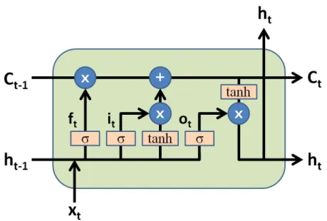
Figure 1.1: An LSTM block. At time stept,Ctand Ct−1 represent the current and previous
cell states,ht andht−1 represent the current and previous hidden states, ft represents forget
gate, it represents input gate, and ot represents output gate.
variable-length sequences, and more important, RNNs consider all contexts from the past to make a decision about the current frame, which is a desirable property since contextual information plays an important role in sequence modeling.
One challenge in training RNNs is that long-term dependencies cause vanishing gradients, i.e. the magnitude of gradients turns to be very small in long sequences, making recurrent network architectures difficult to optimize. To address this issue, the Long Short Term Memory (LSTM) block was proposed in [HS97] to replace the traditional RNN block.
1.2.3.1 LSTM RNNs
A diagram of an LSTM block is shown in Figure 1.1. A key modification in the LSTM is the memory cell, which maintains history information through time. Nonlinear gates modeled by sigmoid function are introduced to control the information flow. Forget gate ft controls
the information from previous cell state Ct−1. Input gate it controls the new information
generated by non-linear tanh layer. Two information are combined to create an updated cell stateC. Finally, output gate o is used to control the final information outputted to hidden
state ht.
1.3
Speech processing and feature extraction
The raw representation of speech data is a continuous waveform. To effectively perform recognition, speech waveform is first preprocessed using a feature extractor. A standard feature extractor processes segments of speech waveform every 10 ms using a sliding window of 25 ms. These segments are then converted into feature vectors by using different feature extraction methods. Examples of speech features are Mel-filterbank features, Mel-frequency cepstral coefficients (MFCCs) [DM80] and perceptual linear predictions (PLP) [Her90].
1.4
Speaker Verification
Speaker Verification (SV) is to verify, given a voice sample and an associated claim, if the talker is indeed the one he or she claims to be. SV has found wide applications in telephone-based financial transactions, information retrieval from speech databases, voice-based user authentication, etc. For SV, the speech input can be either totally unconstrained (text independent) or constrained to be a known phrase (text dependent). This dissertation considers the more challenging text-independent case. The success of SV systems depends on extracting and modeling speaker-dependent characteristics from speech signals which can effectively distinguish one talker from another.
1.4.1 I-vector/PLDA system
The state-of-the-art text-independent speaker verification system is based on the i-vector framework [DKD10]. In these systems, a universal background model (UBM) is used to collect sufficient statistics for i-vector extraction, and a probabilistic linear discriminant analysis (PLDA) backend is adopted to obtain the similarity scores between i-vectors. There are two different ways to model a UBM: using unsupervised-trained Gaussian mixture models (GMMs) or using a deep neural network (DNN) trained as a phoneme classifier. Therefore, we
will introduce both the I-vector GMM and I-vector DNN systems as well as PLDA modeling.
1.4.1.1 I-vector GMM system
For an I-vector GMM system, both speaker model and speaker-independent background model (i.e. UBM) are represented by GMMs. By concatenating the means of these Gaussian mixtures, GMM supervectors could be generated to represent different speakers. The i-vector representation here is based on the total variability modeling concept which assumes that speaker- and channel- dependent variabilities reside in a low-dimensional subspace, represented by the total variability matrix T. Mathematically, the speaker- and channel-dependent GMM supervector s can be modeled as:
s=s0+T w (1.6)
where s0 is the speaker- and channel-independent supervector generated from UBM, T is a rectangular matrix of low rank and w is a random vector called the i-vector which has a standard normal distributionN(0, I).
In order to learn the total variability subspace, Baum-Welch statistics are computed for a given utterance, and are defined as:
Nc = X t P(c|yt,Ω) (1.7) Fc= X t P(c|yt,Ω)yt (1.8)
where Nc and Fc represents the zeroth and first order statistics, yt is the feature sample at
time index t, Ω represent the UBM of C mixture components, c = 1, ..., C is the Gaussian index and P(c|yt,Ω) corresponds to the posterior of mixture component c generating the
1.4.1.2 I-vector DNN system
As mentioned in the previous subsection, for an I-vector GMM system, the posterior of mixture component c generating the vector yt is computed with a GMM acoustic model
trained in an unsupervised fashion (i.e. with no phonetic labels).
P(c|yt,Ω)⇒P(c|yt,Θ) (1.9)
However, recently, inspired by the success of DNN acoustic models in automatic speech recognition (ASR), [LSF14] proposed a method which uses DNN senone (cluster of context-dependent triphones) posteriors to replace the GMM posteriors as illustrated in Eq.1.9, which leads to significant improvement in speaker verification. Θ represents the trained DNN model for senone classification.
The senone posterior approach uses ASR features to compute the class soft alignment and the standard speaker verification features for sufficient statistic estimation. Once sufficient statistics are accumulated, the training procedure is the same as in the previous section. In this dissertation, we use a state-of-the-art time delay neural network (TDNN) as in [PPK15] to train the ASR acoustic model.
1.4.1.3 PLDA modeling
PLDA is a generative model of i-vector distributions for speaker verification. In this disser-tation, we use a simplified variant of PLDA, termed as G-PLDA [KSO13], which is widely used by researchers. A standard G-PLDA assumes that the i-vector wi is represented by:
wi =r+U x+i (1.10)
whereris the mean of i-vectors,U defines the between-speaker subspace, and the latent vari-able xrepresents the speaker identity and is assumed to have standard normal distribution. The residual term i represents the within-speaker variability, which is normally distributed
PLDA based i-vector system scoring is calculated using the log likelihood ratio (LLR) between a target and test i-vectors, denoted aswtarget and wtest. The likelihood ratio can be
calculated as follows:
LLR= log P(wtarget, wtest|H1)
P(wtarget|H0)P(wtest|H0)
(1.11) where H1 and H0 denote the hypothesis that two i-vectors represent the same speaker, and
different speakers, respectively.
1.4.2 Speech corpora
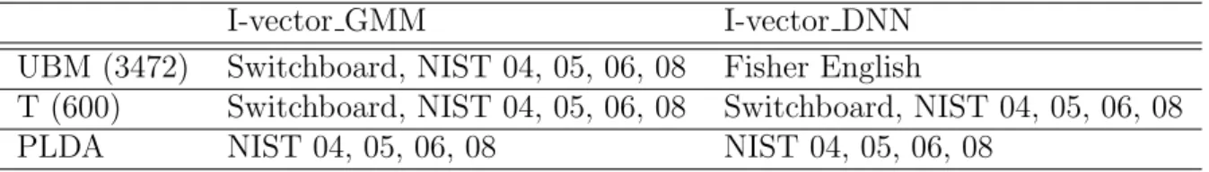
Four speech corpora are used for the SV experiments in this dissertation. A brief overview of each speech corpus will be described in the following subsections.
1.4.2.1 NIST SRE
The NIST Speaker Recognition Evaluation (SRE) is a series of evaluations designed for text independent speaker recognition research [DPM00]. Dataset we used in this dissertation includes SRE 2004, 2005, 2006, 2008 and 2010. SRE datasets contain thousands of hours of speech collected from several thousands speakers. They also cover a variety of channels and conditions, including telephone and microphone speech.
1.4.2.2 Switchboard-2
Switchboard-2 (SWB-2) data was collected by Linguistic Data Consortium (LDC) in support of speaker recognition projects, and it contains several thousands telephone conversations. SWB-2 Phase II was used in this dissertation.
1.4.2.3 SITW
The Speakers in the Wild (SITW) speaker recognition database [MFC16] contains hand-annotated speech samples from open-source media for the purpose of benchmarking
text-independent speaker recognition technology on single and multi-speaker audio acquired across unconstrained or wild conditions. The database consists of recordings of 299 speak-ers, with an average of eight different sessions per person. This data contains real noise, reverberation, intraspeaker variability and compression artifacts.
1.4.2.4 WashU-UCLA
WashU-UCLA dataset [ALS15] contains time-synchronized recordings of speech and sub-glottal acoustics obtained from 25 male and 25 female adult native speakers of American English. Recordings of time-synchronized speech and subglottal acoustics were made with a microphone and an accelerometer, respectively.
1.4.3 Evaluation metrics
For SV, each test utterance and enrolled speaker model comparison is referred to as a trial. As a binary classification task, given a threshold vale, false acceptance rate (RF A) and
false rejection rate (RF R) defined in 1.12 and 1.13 can be used to evaluate performance.
A detection error tradeoff (DET) curve can be created by plotting RF A versus RF R given
different threshold values.
RF A =
Number of False Acceptance
Number of impostor accesses (1.12)
RF R =
Number of False Rejection
Number of target accesses (1.13)
In order to quantify the performance, two most popular metrics (i.e. equal error rate (EER) and minimum detection cost function (minDCF)) are calculated based on the DET curve. EER corresponds to the point on DET curve where RF A and RF R are equal. The
detection cost function is defined in 1.14 as a weighted sum of RF A and RF R,
where CF R and CF A are cost defined by the evaluation plans, and Ptarget and Pimpostor are
the prior probability of the specified target or impostor speaker. minDCF is the minimum value of DCF.
1.5
Automatic Speech Recognition
Figure 1.2: A standard ASR system.
1.5.1 DNN-HMM based speech recognition system
Automatic Speech Recognition (ASR) is the process of transcribing human speech into text automatically using machines. Figure 1.2 shows the components of a typical speech recogni-tion system, which we will describe briefly. An input audio recording is first processed using a feature extractor to generate acoustic features, and then the extracted features are used by an Acoustic Model (AM). The acoustic model is a statistical model of the features condi-tioned on different spoken sound classes. Sound classes are usually represented by states in
mixture models (GMMs) or neural network models, e.g. a Deep Neural Network (DNN), Convolutional Neural Network (CNN), or Recurrent Neural Network (RNN).
After acoustic modeling, Decision Trees map sub-word units (the hidden states generated by an HMM) to phoneme sequences. Then, the Lexicon, or Pronunciation Model, maps a sequence of phonemes to a word.
The Language Model (LM) is a statistical model giving the probability of word sequences independent of the acoustics. The standard language models used in ASR are n-grams. N-gram models represent the probability of generating the next word given the previous N-1 words. The log probability from the language model is typically linearly combined with the acoustic model score, and then fed into the decoder.
The decoder combines the probabilities from the AM and LM to search for the best word sequences under the constraints of the pronunciation model. Most decoders use a combination of dynamic programming and beam-searching to generate a subset of plausible candidates, and score them at the same time. Modern decoders are usually implemented using Weighted Finite State Transducers (WFSTs) for efficient searching.
We now describe the AM and LM parts in a standard state-of-the-art DNN-HMM speech recognition system with formal mathematical notation.
1.5.1.1 Acoustic model
Given the observation sequence (feature frames), X, extracted from a speech waveform, we want to find the best word sequence Wˆ that maximizes the posterior probability p(W|X):
ˆ
W= argmax
W
p(W|X) (1.15)
We can decompose this probability into two terms using Bayes’s Rule, an acoustic model,
pAM(X|W), and a language model,pLM(W):
ˆ
W= argmax
W
In the traditional Gaussian Mixture Model-Hidden Markov Model (GMM-HMM) paradigm, the output probabilities are generated by the GMM, and the sequential property of speech is modeled by the HMM. The hidden states, S, in the HMM typically represent a subword or phonetic segmentation of a word. Therefore we would change pAM(X|W) in Eq.1.16 to:
pAM(X|W) = X S p(X,S|W) =X S p(X|S,W)p(S|W) =X S Y t p(xt|st)p(S|W) (1.17)
where xt and st are the observation and hidden state at time t, respectively. The first
term p(xt|st) in Eq.1.17 is modeled by GMMs, which evaluate the likelihood of a speech
observation xt being generated by a hidden state st.
In practice, HMM hidden states are typically modeled by 3-state triphones. A triphone is a phone with a left and right context. Each triphone is usually modeled by 3 left-to-right states to handle transient acoustic dynamics. Systems that model triphones are usually referred to as having context dependent (CD) models, while systems that model just single phonemes without any context use context independent (CI) models.
The parameters of the GMM-HMM acoustic model can be estimated using Maximum Likelihood Estimation (MLE) and the Forward-Backward algorithm. Details can be found in [RJR93].
A DNN-HMM system usually starts with a baseline GMM-HMM speech recognizer that computes frame-level output target labels. This is usually done by force aligning the tran-scription with the input speech by the GMM-HMM recognizer. Then, a DNN is used to model the posterior probability of an acoustic frame xt being in state st:
Since DNNs produce posteriors but the HMM requires the likelihood p(xt|st) during the
decoding process (as shown in Eq.1.17), we need to convert the DNN outputs to likelihoods:
p(xt|st) =
p(st|xt)p(xt)
p(st)
(1.19)
p(st) is the prior probability of statestestimated from the training set. p(xt) is
indepen-dent of the word sequence and thus can be ignored. In this approach, HMMs are still used to model transition probability and perform sequence modeling, and therefore, DNN-HMM is usually called the hybrid model.
1.5.1.2 Language model
A language model, pLM(W) in Eq. 1.16, can be decomposed as:
pLM(W) = p(w1, w2, ..., wm) = p(w1)p(w2|w1)· · ·p(wm|w1, ..., wm−1) (1.20)
Each of these conditional probabilities could be estimated by checking counts of word se-quences (w1, w2, ..., wi) and (w1, w2, ..., wi−1) in the training corpus:
p(wi|w1, ..., wi−1) =
c(w1, w2, ..., wi)
c(w1, w2, ..., wi−1)
(1.21)
As mentioned before, the classic technique to model LM for ASR are n-grams. An n-gram language model has the Markovian assumption, conditioning on the previous n−1 word, i.e.:
p(wi|w1, ..., wi−1) =p(wi|wi−(n−1), ..., wi−1) (1.22)
In real applications, 2- to 5-word history is typically used for an n-gram model, and, therefore, it will lose long-range context dependency. Recently, researchers have considered using RNNs for language modeling as well. However, due to the computational cost, LMs based on RNNs are typically used to re-score the N-best lists after the beam search is completed. LMs are usually trained independently from the AMs on a large amount of text data.
1.5.2 End-to-end speech recognition system
In the previous subsection, we described DNN-HMM hybrid ASR systems, which are com-posed of several individual components: acoustic models, pronunciation models, and lan-guage models. Each module is trained separately with different criteria, which may not be optimal for the overall task. Therefore, several end-to-end ASR models have been proposed in the last few years.
Connectionist Temporal Classification (CTC) model [GFG06] is one such end-to-end model, which can directly transform a variable acoustic sequence into English characters. The model can be optimized using a CTC loss. CTC models have been shown to learn pro-nunciations model directly. However, CTC models still suffer from conditional independence assumptions and must rely on explicit language models during decoding.
In the Chapter 4 of this dissertation, we focus on attention-based sequence-to-sequence models for end-to-end ASR, which are able to fold separate models of a conventional ASR system into a single neural network, and not be restricted by the independence assumptions of HMM and CTC models. Listen, Attend and Spell (LAS) [CJL16] is one of such models, and it offers improvements over other sequence-to-sequence models as shown in previous work [PRS17].
Let x = (x1, ..., xT) be the input sequence of audio frames, and y = (y1, ..., yS) be the
output sequence of text units (such as characters, words or subwords). The LAS model predicts each output yi using a conditional distribution over the previously emitted output
y<i and the input acoustic sequence x. The LAS model consists of three sub-modules as
shown in Figure 1.3: an encoder which is analogous to a conventional acoustic model, an attender that does alignment, and a decoder that is analogous to the language model.
The encoder (the Listen function) transforms the original feature sequence xinto a high level representation h. The attender and decoder (the AttendandSpell function) take h as input and produce a distribution over text unit sequences:
Figure 1.3: Components of the LAS model.
h = Listen(x) (1.23)
p(y|x) = AttendAndSpell(h) (1.24) The Listen function can be LSTM networks or stacked CNN and LSTM networks. The AttendAndSpell function is an attention-based transducer:
si = DecoderRNN(yi−1, ci−1, si−1) (1.25)
ci = AttentionContext(si,h) (1.26)
p(yi|x,y<i) = TokenDistribution(si, ci) (1.27)
The DecoderRNN function produces a transducer state si as a function of the previously
emitted token yi−1, the previous attention context ci−1 , and the previous transducer state
The AttentionContext function generates context ci with a fully-connected attention
network. It first predicts the attention scores for current transducer state si with each of
the hidden vector in h. The attention scores act as alignments between output text unit and input frames. The attention context ci is then created as a weighted linear sum of h
using the attention scores. The TokenDistribution function is a fully-connect nework with softmax outputs modeling the text unit distribution p(yi|x,y<i).
1.5.3 Speech corpora
Three speech corpora are used for the ASR experiments in this dissertation. A brief overview of each speech corpus will be described in the following subsections.
1.5.3.1 Fisher English
Fisher English dataset [CMW04] is a conversational telephone speech dataset for large vo-cabulary continuous speech recognition (LVCSR). It contains time-aligned transcript data for 11699 complete conversations, each lasting up to 10 mins (in total around 2000 hours).
1.5.3.2 Wall Street Journal
The Wall Street Journal (WSJ) [PB92] speech corpus contains read speech of articles drawn from the Wall Street Journal text corpus. The corpus has rich diversity of voice quality and dialect. The speech data was recorded using microphones with 16kHz sampling rate. In this dissertation, 80 hours’ speech data is used.
1.5.3.3 LibriSpeech
The LibriSpeech corpus [PCP15] is an ASR corpus based on public domain audio books. The corpus is derived from LibriVox’s audio books, and contains around 1000 hours of read speech sampled at 16 kHz.
1.5.4 Evaluation metrics
In order to compare ASR hypothesis and ground-truth transcription, word error rate (WER) is introduced to evaluate recognition accuracy. WER measures the rate of word errors in ASR hypothesis, which is computed as:
W ER = S+D+I
N (1.28)
where S, D and I are the number of substitutions, deletions and insertions, respectively.
N is the number of words in the reference (transcription). Computation of WER requires aligning each hypothesized word sequence with the reference using dynamic programming.
1.6
Dissertation Outline
The rest of this dissertation is organized as follows:
Chapter 2 presents two novel neural-network based representation learning approaches for short-utterance speaker verification. Results on large SV databases are presented and the effectiveness of speaker representation learning using the proposed approaches is analyzed.
Chapter 3 investigates joint feature extraction and acoustic modeling using unified neural-network models. Several novel neural-neural-network architectures are presented, where complex DFT or raw waveforms constitute the input. Experimental results are presented for a large-scale keyword spotting task and a large-vocabulary ASR task.
Chapter 4 proposes two novel neural-network models for sequence modeling. An acoustic-sequence model is presented for an acoustic scene classification task, and then a acoustic- sequence-to-sequence based text-error correction model is proposed for an end-to-end ASR system.
Chapter 5 summarizes the key concepts and results of this dissertation, and provides suggestions for future work.
CHAPTER 2
Learning speaker representations from short utterances
2.1
Introduction
As mentioned in Chapter 1, the i-vector based framework has defined the state-of-the-art for text-independent speaker recognition systems. The i-vector/ PLDA systems perform well if long (e.g. more than 30 s) enrollment and test utterances are available, but the performance degrades rapidly when only limited data are available [KVD11]. However, the requirement of significant amounts of speech for evaluation, has limited the potential of its widespread practical implementations. A speaker verification system, in the real world, is constrained by the amount of speech data.
To address this issue, in this chapter, we present two novel neural-network based repre-sentation learning approaches for short-utterance speaker verification. The fundamental idea is to alleviate possible phoneme mismatch in text-independent short utterance situatitons.
We first propose a method to use a deep neural network to estimate subglottal features from speech signals by leveraging the speaker specificity and stationarity of subglottal acous-tics, which are largely phoneme independent. This work was published in [GYM16]. We then propose an i-vector mapping approach using deep neural networks, which maps the short ut-terance i-vector to its long version. Full-length (more than 30sec-length utut-terance) i-vectors have much smaller variations compared with i-vectors extracted from short utterances. The work was partially published in [GNA17, GXQ18].
2.2
Related work
There has been a number of methods to learn speaker representations from short utter-ance. Recently, several approaches have been proposed which use deep neural networks to learn speaker embeddings from short utterances. In [SGP17], the authors use a neural network, which is trained to discriminate between a large number of speakers, to generate fixed-dimensional speaker embedding, and the speaker embedding are used for PLDA scor-ing. In [ZK17], the authors propose an end-to-end system which directly learns a speaker discriminative embedding using a triplet loss function and an Inception Net [SLJ15]. Both methods show improvement over GMM-based i-vector systems. A few recent papers have also focused on i-vector mapping, which maps the short utterance i-vector to its long version. In [KMA18], the authors proposed a probabilistic approach, in which a GMM-based joint model between long and short utterance i-vectors was trained, and a minimum mean square error (MMSE) estimator was applied to transform a short i-vector to its long version. How-ever, the proposed mapping function is actually a weighted sum of linear functions, which may not be complex enough to model this mapping.
2.3
Learning speaker-specific and phoneme-invariant subglottal
acoustic features
2.3.1 Subglottal acoustic features
Our previous research indicates that subglottal acoustics (capturing the acoustics of the trachea-bronchial airways) are speaker specific and their spectral characteristics are much less variable than the spectral characteristics of speech waveforms [Guo15, GYA17, GPY15]. Subglottal acoustic data were recorded by a noninvasive accelerometer attached to the skin of the neck below the thyroid cartilage. The recordings constitute the WashU-UCLA database [ALS15]. The database consists of 35 monosyllables (14 hVd and 21 CVd words, where V includes all the American English monophthongs and diphthongs) in a phonetically neutral carrier phrase (I said a again), with 10 repetitions of each word by each speaker. The corpus
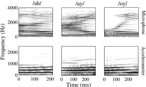
Figure 2.1: Spectrograms of three vowels by a female speaker to compare within-speaker variability of microphone speech (top panel) and subglottal acoustics (bottom panel). Note that the subglottal acoustics don’t vary much. Data are sampled from the recordings of a female speaker in the WashU-UCLA corpus.
has simultaneous microphone and (subglottal) accelerometer recordings of 25 adult male and 25 adult female speakers of American English, and in total 17500 individual microphone (and accelerometer) waveforms. Figure 2.1 exemplifies the stationarity of subglottal acoustics using spectrograms of vowels and their corresponding recordings of subglottal acoustics. The stationary nature of subglottal acoustics can be particularly beneficial when the amount of speech data is limited.
2.3.2 Proposed estimation method
Estimating subglottal features using speech signals is challenging. DNNs have been shown to be effective for feature mapping of speech signals [HHB15]. We adopt DNNs here for subglottal feature estimation and evaluate the technique on the WashU-UCLA corpus (which contains time-synchronized recordings of speech and subglottal acoustics). We train a DNN regression model to learn the spectral feature mapping from speech to subglottal acoustics. The objective function for optimization is based on the mean square error. Eq. 2.1 is the
cost function for each training batch: Lr(xk, yk;θr) = 1 N N X k=1 kyk−f(xk)k2 (2.1)
where xk and yk are the input speech feature and the corresponding subglottal acoustic
feature, respectively, andθr denotes the regression parameters to be learned during training.
The trained DNN regression model f(.) provides a non-linear mapping from a more variable speech spectral domain to the less variable subglottal spectral domain (viewed in some sense as a many-to-one mapping).
2.3.3 Estimation experiments
2.3.3.1 Feature extraction and DNN mapping setup
To avoid redundancy and keep the phonetic balance in the data that is used to train the DNN regression model, only the vowel segments of the monosyllables in the database are isolated and used. Another reason why we only extract the vowel segments is that the accelerometer signals show little information for consonants. Since we only have the DNN mapping for vowels, we need a way to deal with non-vowel segments while estimating subglottal acoustic features for the speaker verification experiment. Section 2.3.4 explains the specific method used for that.
We extract the 40 dimensional log Mel-filterbank coefficients for both speech and ac-celerometer segments, and use the filterbank feature vectors of the speech segments as input and their corresponding subglottal filterbank feature vectors as output for the DNN model. The input and output features are normalized using the L2 norm of the feature vector. The activation functions of both the hidden layers and the output layer are the tanh functions. Three hidden layers are used and each hidden layer has 256 neurons. We use backpropagation with mini-batch stochastic gradient descent to train the DNN model, and the optimization technique uses adaptive gradient descent along with a momentum term. The THEANO DNN toolkit is used for DNN training [BLP12]. All available vowel segment pairs (17500 in
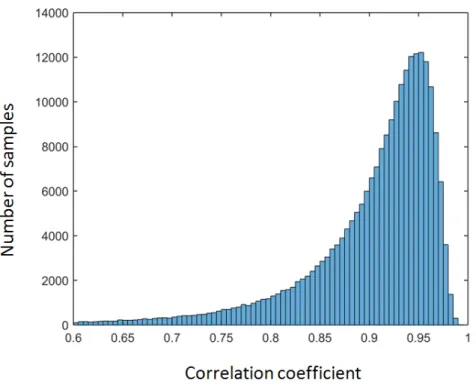
Figure 2.2: Histogram of the correlation coefficient of the actual and estimated subglottal Mel-filterbank coefficients for each frame in the validation dataset.
total) are split into a training set and a validation set. The training set has roughly 80% of the data and the rest is for validation. All signals are down sampled to 8 kHz (from the original sampling rate of 48 kHz), which is consistent with the NIST SRE dataset (used for speaker verification). The log Mel-filterbank coefficients for both speech and subglottal acoustic signals are extracted at 10ms intervals using a 20 ms Hamming window.
2.3.3.2 Evaluation results
To evaluate the performance of the DNN-based estimation model, we use two methods: (1) computing the correlation between actual and estimated log Mel-filterbank coefficients for each frame of subglottal recordings, and (2) comparing the actual and estimated subglottal features with regards to their ability to discriminate between speakers.
Figure 2.2 shows the histogram of the correlation coefficients for all frames in the vali-dation dataset. The average value of the correlation coefficients is 0.9, which indicates the sufficiency of the DNN-based estimation model.
Feature sets J-Ratio MFCCs (x1-x20) 4.92
Actual SGCCs (x1-x20) 5.48
Estimated SGCCs (x1-x20) 5.47
Table 2.1: J-ratio, a measure of class separation for different feature values. Features were extracted from isolated vowel recordings of speech and subglottal acoustics, for all the 50 male and female adult speakers in the WashU-UCLA corpus.
To compare the actual and estimated subglottal filterbank features in terms of speaker discriminability, the J-Ratio [Fuk13], which measures class separation, is used. Before cal-culating the J-Ratio, we compute the DCT of the log Mel-filterbank coefficients, since it will decorrelate the filterbank features and be consistent with MFCC features (used commonly for speaker verification tasks). We refer to the subglottal features after taking the DCT on the log Mel-filterbank coefficients as subglottal cepstral coefficients, which are denoted as SGCCs. The zeroth cepstral coefficient is discarded, since it only captures the energy information. The first 20 coefficients are used for both MFCCs and SGCCs. Given feature vectors for N speakers, the J-Ratio can be computed using Eqs. 2.2-2.4:
Sw = 1 MΣ M s=1Ri (2.2) Sb = 1 MΣ M s=1(xi−xo)(xi−xo)T (2.3) J = Tr((Sb+Sw)−1Sb) (2.4)
where Sw is the within-class scatter matrix, Sb is the between-class scatter matrix, xi is
the mean feature vector for theithspeaker,xo is the mean of allxis, andRi is the covariance
matrix for the ith speaker (a higher J-Ratio means better separation).
Table 2.1 shows the J-Ratio values for different feature sets. The results show that: (1) SGCCs offer better separation compared to MFCCs, which is partly attributable to the
stationarity of subglottal acoustics and the low within-class variance that they represent, and (2) the estimated SGCCs are similar in performance to actual SGCCs, which is due to the effectiveness of the DNN-based feature mapping model.
2.3.4 Speaker verification experiments
2.3.4.1 Task description and experimental settings
We evaluate our features and proposed system on the NIST SRE datasets with state-of-the-art i-vector/PLDA framework. The NIST SRE 2004, 2005, 2006 and Switchboard II datasets are used as the development dataset. Gender-dependent universal background mod-els (UBM) with 2048 Gaussians are trained using a subset of the development dataset, which only has utterances from male speakers. The total variability subspace for the i-vector ex-tractor, channel compensation technique LDA and speaker variability subspace for PLDA are trained using all male speakers from the development dataset. The Kaldi toolkit [PGB11] is used to build the system.
MFCCs using the first 20 coefficients (discarding the zeroth coefficient) with appended first and second order derivatives are extracted from the detected speech segments after voice activity detection. A 20 ms Hamming window, a 10 ms frame shift, and a 23-channel Mel-filterbank are used for baseline MFCC feature extraction. A total variability matrix T of 400 factors is used and the dimension is reduced to 200 using LDA before the PLDA modeling. Length normalization of the ivectors is also used.
For SGCC feature extraction, non-vowel speech frames must be discarded since the DNN feature extractor is trained only on isolated vowels. A normalized autocorrelation peak value of 0.7 is used as a threshold to detect the strongly-voiced vowel frames. A 20 ms Hamming window and a 10 ms frame shift are used to extract 40-channel Mel-filterbank coefficients from voiced frames. Then, the filterbank coefficients are inputted into the trained DNN feature extractor to estimate subglottal features. The first 20 coefficients (excluding the zeroth coefficient) with appended first order derivatives are selected after taking the DCT on the estimated subglottal Mel-filterbank coefficients. A total variability subspace of 150
Figure 2.3: Block diagram of the proposed framework.
dimensions is used and the same number of latent components is adopted for PLDA modeling. Length normalization is also done to scale the lengths of each i-vectors to unit length.
The NIST SRE 2008 core task, which has both microphone and telephone speech and channel matched and mismatched conditions, was used for the experiments. The enrollment and testing datasets are truncated to 10 seconds and 5 seconds for each utterance for the short-utterance speaker verification tasks. The core task contains 1993 female and 1270 male speakers. Only the male speakers with 39433 test trials are used here for evaluation. We show the results for conditions C2 (interview speech from the same microphone types for both training and testing), C7 (English telephone speech spoken by both native and non-native U.S. English speakers), and C8 (English telephone speech spoken by native U.S. English speakers). These conditions were chosen because they contain English-only speech. Given an utterance, MFCCs and SGCCs are computed as described earlier. Each feature set will generate a set of scores for test trials. Scores from the two speaker verification systems were normalized to the range (0, 1) and fused in a linearly-weighted fashion such that the weights sum up to 1. The fused scores are used to make final decisions. The overall block diagram of the framework is presented in Figure 2.3.
2.3.4.2 Results and analysis
While the J-Ratio analysis in Section 2.3.3.2 shows that the estimated SGCCs can provide better speaker separation than MFCCs using the selected vowel segments, initial experiments
Conditions Feature set C2 C7 C8 10sec-10sec MFCCs 8.12 19.51 21.08 MFCCs+SGCCs 7.20 18.24 19.29 Relative improvement 11.5% 6.5% 8.5% 5sec-5sec MFCCs 14.11 27.76 27.83 MFCCs+SGCCs 12.10 26.21 26.07 Relative improvement 14.3% 5.6% 6.3%
Table 2.2: EERs for the MFCC baseline system and the fused system on the NIST SRE 08 truncated 10sec-10sec and 5sec-5sec evaluation tasks. The relative improvements in EERs are also shown.
indicate that the SGCC-only system performs worse than the MFCC baseline on the NIST SRE dataset. This discrepancy could be due to (1) acoustic mismatch between the WashU-UCLA corpus and the speaker verification corpora, and (2) using only the strongly-voiced frames for SGCC estimation.
Therefore, we further investigate the performance of fused MFCCs+SGCCs systems in Table 2.2, to examine if they are complementary to each other. The fused system gives improvement for all conditions of the short-utterance task. The gains are higher and more significant for the conditions that better match the characteristics of the WashU-UCLA corpus used for DNN training. For example, the combined system yields the biggest im-provement under matched microphone speech (C2), with a relative 11.5% EER reduction for the 10sec-10sec task, and 14.3% for the 5sec-5sec task. This may be due to the fact that the DNN mapping model is also trained under matched microphone speech. For English telephone speech, we can see that C8, which contains utterances spoken by Native American English speakers, gives relative better improvement compared with C7. This may also result from the fact that all the speakers in the WashU-UCLA dataset are native US speakers. The weights used for fusion are the same for both 10sec-10sec and 5sec-5sec tasks, which are 0.85 for MFCCs and 0.15 for SGCCs.
2.4
Learning non-linear mapping from short-utterance to
long-utterance i-vectors
The previous section investigates the method of learning speaker-specific and phoneme-invariant features at the frame level. In this section, we will explore an approach of learning phoneme-invariant speaker features through utterance-level representations.
2.4.1 The effect of utterance durations on i-vectors
Full-length i-vectors have relatively smaller variations compared with i-vectors extracted from short utterances, because i-vectors of short utterances can vary considerably with changes in phonetic content. In order to show the variation changes between long and short utterance i-vectors, we first calculate the average diagonal covariance (denoted asσm) of i-vectors across
all utterances of a given speaker m and then calculate the mean (denoted as σmean) of the
covariances over all speakers. σm and σmean are defined in as:
σm = 1 NΣ N n=1Tr((wmn−w¯m)(wmn−w¯m)T) (2.5) σmean = 1 MΣ M m=1σm (2.6)
where ¯wm corresponds to the mean of the i-vectors belonging to speaker m. N represents
the total number of utterances for speaker m, Tr(.) represents the trace operation, and M
is total number of speakers.
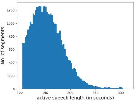
In order to compare the σmean for long and short utterance i-vectors, we choose around
4000 speakers with multiple long utterances (more than 2 min in duration and 100 s of active speech) from the SRE and Switchboard-2 (SWB-2) datasets (in total around 40000 long utterances) and truncate each long utterances into multiple 5-10 s short utterances. We plot the distribution of active-speech length (utterance length after voice activity detection) across these 40000 long utterances in Figure 2.4. From the figure, we can observe that the
Figure 2.4: Distribution of active speech length of 40000 long utterances in SRE and SWB datasets.
Table 2.3: Mean variance of long and short utterances (from the SRE and Switchboard datasets)
i-vectors
long utterance short utterance mean variance(σmean) 283 493
majority of the utterances have active-speech length between 100-250 s. The i-vectors are then extracted for each short and long utterance using the I-vector DNN system. Table 2.3 shows the mean variance σmean across all speakers calculated from long and short utterance
i-vectors. The mean of the variances in the Table 2.3 indicates that short-utterance i-vectors, as expected, have larger variation compared to those of long-utterance i-vectors.
2.4.2 DNN-based i-vector mapping
In order to alleviate possible phoneme mismatch in text-independent short utterances, we propose several methods to map short-utterance i-vectors to their long versions. This map-ping is a many-to-one mapmap-ping, from which we want to restore the missing information from
the short-utterance i-vectors and reduce their variance.
In this section, we will introduce and compare several novel DNN-based i-vector mapping methods. Our pilot experiments indicate that, if we train a supervised DNN to learn this mapping directly, similar to the approaches in [BR17] , the improvement is not significant due to over-fitting to the training dataset. In order to solve this problem, we propose two different methods which model the joint representation of short and long utterance i-vectors by using an autoencoder. The decoder reconstructs the original input representation and forces the encoded embedding to learn a hidden space which represents both short and long utterance i-vectors and thus can lead to better generalizations. The first is a two-stage method: use an autoencoder to first train a bottleneck representation of both long and short utterance i-vectors, and then use pre-trained weights to perform a supervised fine-tuning of the model, which maps the short-utterance i-vector to its long version directly. The second is a single-stage method: jointly train the supervised regression model with an autoencoder to reconstruct the short i-vectors. The final loss to optimize is a weighted sum of the supervised regression loss and the reconstruction loss. In the following subsections, we will introduce these two methods in detail.
2.4.2.1 DN N1 (two-stage method): pre-training and fine-tunning
In order to find a good initialization of the supervised DNN model, we first train a joint representation of both short and long utterance i-vectors using an autoencoder. The autoen-coder consists of an enautoen-coder and a deautoen-coder as illustrated in Figure 2.5. We first concatenate the short i-vector ws and its long versionwl intoz as input. The encoder function h=f(z)
learns a hidden representation of input vector z, and the decoder function ˆz = g(h) pro-duces a reconstruction. The learning process is described as minimizing the loss function
L(z, g(f(z))). The autoencoder learns the joint hidden representation of both short and long i-vectors, which leads to good initialization of the second-stage supervised fine-tuning. In order to learn a more useful representation, we add a restriction on the autoencoder: con-strain the hidden representationh to have a relatively small dimension in order to learn the
Figure 2.5: DN N1: two-stage training of i-vector mapping. Left schema corresponds to the
first-stage pre-training. A short-utterance i-vector ws and a corresponding long-utterance
i-vector wl are first concatenated into z. Then z is fed into an encoder f(.) to generate the
joint embeddingh. h is passed to the decoder g(.) to generate the reconstructed ˆz, which is expected to be a concatenation of a reconstructed ˆws and ˆwl. Right schema corresponds to
the second-stage fine-tuning. The pre-trained weights in the first stage is used to initialize the supervised regression model from ws to wl. After training, the estimated i-vector ˆwl is
used for evaluation.
most salient features of the training data.
For the encoder function f(.), we adopt options from several fully-connected layers to stacked residual blocks [HZR16], in order to investigate the effect of encoder depth. Each residual block has two fully-connected layers with a short-cut connection as shown in Fig-ure 2.6. By using residual blocks, we are able to train a very deep neural network without adding extra parameters. A deep encoder may help learn better hidden representations. For a decoder function g(.), we use a single fully-connected layer with a linear regression layer, since it is enough to approximate the mapping from the learned hidden representation h to the output vector. For the loss function, we use the mean square error criterion, which is
kg(f(z))−zk2.
Once the autoencoder is trained, we use the trained DNN-structure and weights to ini-tialize the supervised mapping. We optimize the loss between the predicted long i-vector and the real long i-vector N1 PN
n=1kwˆl−wlk2 as shown in Figure 2.5. We denote this method