A simple multi-class boosting framework with theoretical guarantees and empirical proficiency

(1)

with Theoretical Guarantees and Empirical Proficiency

Ron Appel1 Pietro Perona1

Abstract

There is a need for simple yet accurate white-box learning systems that train quickly and with lit-tle data. To this end, we showcase REBEL, a multi-class boosting method, and present a novel family of weak learners called localized similar-ities. Our framework provably minimizes the training error of any dataset at an exponential rate. We carry out experiments on a variety of synthetic and real datasets, demonstrating a con-sistent tendency to avoid overfitting. We eval-uate our method on MNIST and standard UCI datasets against other state-of-the-art methods, showing the empirical proficiency of our method.

1. Motivation

The past couple of years have seen vast improvements in the performance of machine learning algorithms. Deep Nets of varying architectures reach almost (if not better than)human performance in many domains (LeCun et al.,

2015). A key strength of these systems is their ability to transform the data using complex feature representations to facilitate classification. However, there are several con-siderable drawbacks to employing such networks.

A first drawback is that validating through many architec-tures, each of which may have millions of parameters, re-quires a lot of data and time. In many fields (e.g. pathology of not-so-common diseases, expert curation of esoteric sub-jects, etc.), gathering large amounts of data is expensive or even impossible (Yu et al.,2015). Autonomous robots that need to learn on the fly may not be able to afford the large amount of processing power or time required to prop-erly train more complex networks simply due to their hard-ware constraints. Moreover, most potential users (e.g. non-machine-learning scientists, small business owners,

hobby-1

Caltech, Pasadena, USA. Correspondence to: Ron

Appel <[email protected]>, Pietro Perona <

[email protected]>.

(a) Old: Decision Stumps (b) New: Localized Similarities

Figure 1. (a) The typical decision stumps commonly used in boosting lead to classification boundaries that are axis aligned and not representative of the data. Although these methods can achieve perfect training accuracy, it is apparent that they heavily

overfit. (b) Our method useslocalized similarities, a novel family

of simple weak learners (see Sec.5.1). Paired with a procedure

that provably guarantees exponential loss minimization, our clas-sifiers focus on smooth, well-generalizing boundaries.

ists, etc.) may not have the expertise or artistry required to hypothesize a set of appropriate models.

A second drawback is that the complex representations achieved by these networks are difficult to interpret and to analyze. For many riskier applications (e.g. self-driving cars, robotic surgeries, military drones, etc.), a machine should only run autonomously if it is able toexplainits ev-ery decision and action. Further, when used towards the sci-entific analysis of phenomena (e.g. understanding animal behavior, weather patterns, financial market trends, etc.), the goal is to extract a causal interpretation of the system in question; hence, to be useful, a machine should be able to provide a clear explanation of its internal logic.

For these reasons, it is desirable to have a simple white-box machine learning system that is able to train quickly and with little data. With these constraints in mind, we show-case a multi-class boosting algorithm called REBEL and a novel family of weak learners called similarity stumps, leading to much better generalization than decision stumps, as shown in Fig.1. Our proposed framework is simple, effi-cient, and is able to perfectly train onanydataset (i.e. fully minimize the training error in a finite number of iterations).

(2)

The main contributions of our work are as follows: 1. a simple multi-class boosting framework using

local-ized similarities as weak learners (see Sec.3)

2. a proof that the training error is fully minimized within a finite number of iterations (see Sec.5)

3. a procedure for selecting an adequate learner at each iteration (see Sec.5.2)

4. empirical demonstrations of state-of-the-art results on a range of datasets (see Sec.7)

2. Background

Boosting is a fairly mature method, originally formulated for binary classification (e.g. AdaBoost and similar vari-ants) (Schapire, 1990; Freund, 1995; Freund & Schapire,

1996). Multi-class classification is more complex than its binary counterpart, however, many advances have been made in both performance and theory in the context of boosting. Since weak learners come in two flavors, bi-nary and multi-class, two corresponding families of boost-ing methods have been explored.

The clever combination of multiple binary weak learn-ers can result in a multi-class prediction. AdaBoost.MH reduces the K-class problem into a single binary prob-lem with aK-fold augmented dataset (Schapire & Singer,

1999). AdaBoost.MO and similar methods reduce the K-class problem into C one-versus-all binary problems using Error-Correcting Output Codes to select the final hypothesized class (Allwein et al.,2001;Sun et al.,2005;

Li, 2006). More recently, CD-MCBoost and CW-Boost return a K-dimensional vector of class scores, focusing each iteration on a (binary) problem of improving the margin of one class at a time (Saberian & Vasconcelos,

2011;Shen & Hao,2011). REBEL also returns a vector of

class scores, increasing the margin between dynamically-selected binary groupings of theKclasses at each iteration

(Appel et al.,2016).

When multi-class weak learners are acceptable (and avail-able), a reduction to binary problems is unnecessary. Ad-aBoost.M1 is a straightforward extension of its binary counterpart (Freund & Schapire,1996). AdaBoost.M2 and AdaBoost.MR make use of a K-fold augmented dataset to estimate output label probabilities or rankings for a given input (Freund & Schapire,1996;Schapire & Singer,

1999). More recent methods such as SAMME, AOSO-LogitBoost, and GD-MCBoost are based on linear com-binations of a fixed set of codewords, outputting K-dimensional score vectors (Zhu et al., 2009; Sun et al.,

2011;Saberian & Vasconcelos,2011).

In the noteworthy paper “A Theory of Multiclass Boosting”

(Mukherjee & Schapire,2010), many of the existing

boost-ing methods were shown to be inadequate at trainboost-ing; either

because they require their weak learners to be too strong, or because their loss functions are unable to deal with some training data configurations. (Mukherjee & Schapire,

2010) outline the appropriate Weak Learning Condition

that a boosting algorithm must require of its weak learn-ers in order to guarantee training convergence. However, no method is prescribed with which to find an adequate set of weak learners.

The goal of our work is to propose a multi-class boosting framework with a simple family of binary weak learners that guarantee training convergence and are easily inter-pretable. Using REBEL (Appel et al.,2016) as the multi-class boosting method, our framework is meant to be as straightforward as possible so that it is accessible and prac-tical to more users; outlining it in Sec.3below.

3. Our Framework

In this section, we define our notation, introduce our boost-ing framework, and describe our trainboost-ing procedure.

Notation

scalars (regular), vectors (bold): x, x_≡_[_x₁_{, x}₂_{, ...}_]

constant vectors: 0_≡_[0_,₀_{, ...}_]_, 1_≡_[1_,₁_{, ...}_]

indicator vector: δδδk(0with a1in thekth_entry)

logical indicator function: 1(LOGICAL EXPRESSION)∈ {0,1}

inner product: hx_,v_i

element-wise multiplication: x⊙v

element-wise function: F_[x_]_≡_[_F₍_x₁₎_{, F}₍_x₂₎_{, ...}_]

In the multi-class classification setting, a datapoint is repre-sented as a feature vectorxand is associated with a class labely. Each point is comprised ofdfeatures and belongs to one ofKclasses: x_∈X_⊆_Rd_{, y}_∈_Y_{≡ {}₁_,₂_{, ...,K}_}

A good classifier reduces the training error while gener-alizing well to potentially-unseen data. We use REBEL

(Appel et al.,2016) due to its support for binary weak

learn-ers, its mathematical simplicity (i.e. closed-form solu-tion to loss minimizasolu-tion), and its strong empirical perfor-mance. REBEL returns a vector-valued outputH, the sum ofT {weak learnerf, accumulation vectora_}pairs, where ft:X→ {±1} and at∈R K : H(x)≡ T X t=1 ft(x)at

The hypothesized class is simply the index of the maximal entry inH:

F(x)≡arg max

y∈Y{hH(x), δδδyi}

The average misclassification errorεcan be expressed as: ε ≡ _N1

N X

n=1

(3)

REBEL uses an exponential loss function to upper-bound the average training misclassification error:

ε ≤ L ≡ ₂1_N

N X

n=1

hexp[yn⊙H(x_n)],1i (2)

where: yn≡1−2δδδyn (i.e. all+1s with a−1in they th

n index)

Being a greedy, additive model, all previously-trained pa-rameters are fixed and each iteration amounts to jointly op-timizing a new weak learnerf and accumulation vectora. To this end, the loss at iterationI+1can be expressed as:

LI+1= 1 N N X n=1 hwn,exp[f(xn)yn⊙a]i (3) where: wn ≡1 2 exp[yn⊙HI(xn)]

Given a weak learnerf, we define true and false (i.e. correct and incorrect) multi-class weight sums (sT

f andsFf) as: sT f ≡ 1 N N X n=1 1[f(xn)yn<0]⊙wn, sFf ≡ 1 N N X n=1 1[f(xn)yn>0]⊙wn thus: sT f+sFf= 1 N N X n=1 wn, sfT−sFf = 1 N N X n=1 f(xn)wn⊙y_n

Using these weight sums, the loss can be simplified to:

LI+1≡ Lf ≡ hsfT,exp[−a]i+hsfF,exp[a]i (4)

In this form, it is easily shown that with the optimal accu-mulation vectora∗

, the loss has an explicit expression: a∗= 1 2 ln[s T f]−ln[sFf] ∴ L ∗ f = 2h p sT f⊙sfF,1i (5)

At each iteration, growing decision trees requires an ex-haustive search through a pool of decision stumps (which is tractable but time-consuming), storing the binary learner that best reduces the multi-class loss in Eq.5. In some sit-uations, axis-aligned trees are simply unable to reduce the loss any further, thereby stalling the training procedure. Our proposed framework circumvents such situations. At each iteration, instead of exhaustively searching for an ad-equate learner, we first determine an appropriate “binariza-tion” of the multi-class data (i.e. a separation of theK-class data into two distinct groups) and then find a weak learner with a guaranteed reduction in loss, foregoing the need for an exhaustive search.

4. Binarizing Multi-Class Data

At each iteration, the first step in determining an adequate weak learner isbinarizingthe data, i.e. assigning a tempo-rary binary label to each data point by placing it into one of two groups. The following manipulations result in a proce-dure for binarizing datapoints given their boosting weights. Eq.5can be upper-bounded as follows:

L∗f = 2h p sT f⊙sFf,1i ≤ hsTf+sFf,1i − 1 2 U z }| { D_[sT f−sfF]2 [sT f+sFf] ,1E (6) since:px(1−x)≤ 1₂−1₂−x 2 ∀x, using:x= s T sT₊_sF By expandingsT

f±sFf,Uis expressed as a squared norm:

U = *h1 N N P n=1 f(xn)wn⊙y n i2 h₁ N N P n=1 wn i ,1 + = N X n=1 f(xn)un 2 (7) where: un ≡ 1 √ N wn⊙y_n r _N P n=1 wn

Eq.7 can be written as a product of matrices by stacking all of theunas column vectors of aK×N matrixUand

definingf as a row vector with elementsf(xn):

U = f[U⊤U]f⊤

Note that the trace of U⊤U can be lower-bounded:

tr(U⊤U) = N X n=1 kunk2= * N P n=1 [wn]2 Nh N P n=1 wn i,1 + ≥_N12 N X n=1 hwn,1i

since by Jensen’s inequality:

N X n=1 x2 n ≥ 1 N XN n=1 xn 2

Furthermore, U⊤U has N (not-necessarily unique) non-negative eigenvalues, each associated with an independent eigenvector. Letvˆnbe the eigenvector corresponding to the

nth

largest eigenvalueλn. Hence,f can be decomposed as:

f = hf,ˆv1ivˆ1+ N X n=2 hf,vˆniˆvn (8) ∴ U = λ1hf,vˆ1i2+ N X n=2 λnhf,vˆni2 ≥ λ1hf,vˆ1i2

(4)

Since the trace of a matrix is equal to the sum of its eigen-values and U⊤U has at mostKnon-zero eigenvalues (λ1

being the largest), hence: λ1 ≥ 1 Ktr(U ⊤ U) ≥ _KNL0 (9) since: 1 N N X n=1 hwn,1i=L0

Based on this formulation, binarization is achieved by set-ting thebinarized classbnof each samplenas the sign of

its corresponding element invˆ1: bn ≡ sign(hvˆ1, δδδni)

Accordingly, ifbis the vector with elementsbn, then:

hb,vˆ1i2 = hsign[ˆv1],vˆ1i2 = h|ˆv1|,1i2 ≥ 1 (10)

(please refer to supplement for proof)

Finally, by combining Eq.6, Eq.9, and Eq.10, with perfect binarized classification (i.e. when the binary weak learner perfectly classifies the binarized data), the loss ratio at any iteration is bounded by:

Lf∗

L0 ≤

1−₂_KN1

In general, there is no guarantee that any weak learner can achieve perfect binarized classification. In the following section, we show that with the ability toisolateany single point in space (i.e. to classify an inner point as+1and all outer points as−1), the loss decreases exponentially.

5. Isolating Points

Assume that we have a weak learnerfi that can isolate a

single pointxi in the input spaceX. Accordingly, denote

fi = 2δδδi−1 as a vector of−1s with a+1in theithentry,

corresponding to classification using the isolating learner fi(xn). IfN ≥4, then for any unit vector vˆ ∈RN:

max i {hfi,vˆi

2

} ≥ 4

N (11)

(please refer to supplement for proof)

Combining Eq.6, Eq.9, and Eq.11, the loss ratio at each iteration is upper-bounded as follows:

mini{Lfi}

L0 ≤

1−_KN2 2

Before the first iteration, the initial loss L0=K/2. Each

iteration decreases the loss exponentially. Since the train-ing error is discrete and is upper bounded by the loss (as

in Eq.2), our framework attains minimal training error on

any1_{training set after a finite number of iterations:}

define: T0≡ & ln(2/KN) ln 1−KN22 ' ≈ _KN2 2 ln _KN 2 ∴ T ≥T0 ⇒ K 2 1−_KN2 2 T < 1 N ⇒ ε= 0 Although this bound is too weak to be of practical use, it is a bound nonetheless (and can likely be improved). In the following section, we specify a suitable family of weak learners with the ability to isolate single points.

5.1. One/Two-Point Localized Similarities

Classical decision stumps compare a single feature to a threshold, outputting+1or−1. Instead, our proposed fam-ily of weak learners (calledlocalized similarities) compare points in the input space using a similarity measure. Due to its simplicity and effectiveness, we use negative squared Euclidean distance −kxi−xjk2 as a measure of similarity

between pointsxi andxj. A localized similarity has two

modes of operation:

1. In one-point mode, given an anchorxiand a threshold

τ, the input space is classified as positive if it is more

similartoxi thanτ, and negative otherwise; ranging

between+1and−1:

fi(x) ≡ τ− k

xi−xk2

τ+kxi−xk2

2. In two-point mode, given supportsxiandxj, the input

space is classified as positive if it is moresimilar to xi than toxj (and vice-versa), with maximal absolute

activations aroundxiandxj; falling off radially away

from the midpointm: fij(x) ≡ h d,x₋m_i 4kd_k4₊_k_x₋_m_k4 where: d _≡ 1 2[xi−xj] and: m ≡ 1 2[xi+xj]

One-point mode enables the isolation of any single data-point, guaranteeing a baseline reduction in loss. However, it essentially leads to pure memorization of the training data; mimicking a nearest-neighbor classifier. Two-point mode adds the capability to generalize better by provid-ing margin-style functionality. The combination of these

1

There may be situations in which multiple samples belong-ing to different classes are coincident in the input space. These cases can be dealt with (before or during training) either by as-signing all such points as a special “mixed” class (to be dealt with at a later stage), or by setting the class labels of all coincident points to the single label that minimizes the error.

(5)

two modes enables the flexibility to tackle a wide range of classification problems. Furthermore, in either mode, the functionality of a localized similarity is easily interpretable: “which of these fixed training points is a given query point

more similar to?”

5.2. Finding Adequate Localized Similarities Given a dataset withN samples, there are aboutN2

pos-sible localized similarities. The following procedure effi-ciently selects an adequate localized similarity:

0. Using Eq.5, calculate the base lossL1for the homoge-neousstumpf1 (i.e. the one-point stump with anyxi

and τ≡ ∞, classifying all points as+1).

1. Compute the eigenvector vˆ1 (as in Eq. 8); label the

points based on their binarized class labelsbn.

2. Find the optimal isolating localized similarity fi (i.e.

withxiand appropriateτ, classifying pointias+1and

all other points as−1).

3. Using Eq.5, calculate the corresponding lossLi. Of the

two stumpsf1andfi, store the one with smaller loss as

best-so-far.

4. Find pointxj most similar2toxi among points of the

opposite binarized class:

xj = arg min

bj=−bi{k

xi−xjk2}

5. Calculate the loss achieved using the two-point local-ized similarityfij. If it outperforms the previous best,

store the newer learner and update the best-so-far loss. 6. Find all points that aresimilar enoughtoxjand remove

them from consideration for the remainder of the cur-rent iteration. In our implementation, we remove allxn

for which:

fij(xn)≤fij(xj)/2

If all points have been removed, return the best-so-far localized similarity; otherwise, loop back to step 4. Upon completion of this procedure, the best-so-far local-ized similarity is guaranteed to lead to an adequate reduc-tion in loss, based on the derivareduc-tion in Sec.4above.

6. Generalization Experiments

Our boosting method provably reduces the loss well after the training error is minimized. In this section, we demon-strate that the continual reduction in loss serves only to im-prove the decision boundaries and not to overfit the data. We generated 2-dimensional synthetic datasets in order to better visualize and get an intuition for what the classifiers

2 _{“most similar” need not be exact; approximate}

nearest-neighbors also works with negligible differences.

Figure 2. A 500-point 2-dimensional synthetic dataset with a

(2/3,1/3) split of train data (left plot) to test data (right plot).

Background shading corresponds to the hypothesized class using our framework. 100 101 102 103 Iteration [max = 1000] 0 0.2 0.4 0.6 0.8 1

Relative Error, Training Loss

Test Error [%]Test Error [%]Test Error [%]Test Error [%]

log 10 Loss [-20.6] Train Error [0.0%] Test Error [0.0%] 10-30 10-20 10-10 Training Loss 40 102 0 0.2 0.4 0.6 Test Error [%]

Figure 3. A plot of training loss, training error, and test error as a classifier is trained for 1000 iterations. Note that the test error does not increase even after the training error drops to zero. The lower inset is a zoomed-in plot of the train and test error, the upper inset is a plot of training loss using a log-scaled y-axis; both inset plots are congruous with the original x-axis.

are doing. The results shown in this chapter are based on a dataset composed of 500 points belonging to one of three classes in a spiral formation, with a (2/3,1/3) train/test split. Fig.2shows the hypothesized class using a classifier trained for 1000 iterations.

Our classifier achieves perfect training (left) and test classification (right), producing a visually simple well-generalizingcontour around the points. Training curves are given in Fig.3, tracking the loss and classification er-rors per training iteration. Note that the test error does not increase even after the training error drops to zero. The following experiments explore the functionality of our framework (i.e. REBEL using localized similarities) in two scenarios that commonly arise in practice: (1) varying spar-sity of training data, and, (2) varying amounts of mislabeled training data.

(6)

(a4) Train Data (b4) Test Data (c4) Training on4/5of the data (267 points) 100 ₁₀1 ₁₀2 ₁₀3 Iteration [max = 2000] 0 0.2 0.4 0.6 0.8 1

log 10 Loss [-44.2] Train Error [0.0%] Test Error [1.2%] 10-50 Training Loss 50 102 103 0 1 2 3 Test Error [%]

(a3) Train Data (b3) Test Data (c3) Training on3/5of the data (200 points)

100 ₁₀1 ₁₀2 ₁₀3 Iteration [max = 1000] 0 0.2 0.4 0.6 0.8 1

log10 Loss [-22.5] Train Error [0.0%] Test Error [1.8%] 10-30 10-20 10-10 Training Loss 40 102 0 1 2 3 4 Test Error [%]

100 ₁₀1 ₁₀2 ₁₀3 Iteration [max = 5000] 0 0.2 0.4 0.6 0.8 1

log10 Loss [-116.5] Train Error [ 0.0%] Test Error [ 2.0%] 10-150 10-100 10-50 Training Loss 30 102 103 0 5 10 Test Error [%]

100 ₁₀1 ₁₀2 ₁₀3 Iteration [max = 2000] 0 0.2 0.4 0.6 0.8 1

log 10 Loss [ -58.9] Train Error [ 0.0%] Test Error [14.0%] 10-60 10-40 10-20 Training Loss 50 102 103 0 5 10 15 20 Test Error [%]

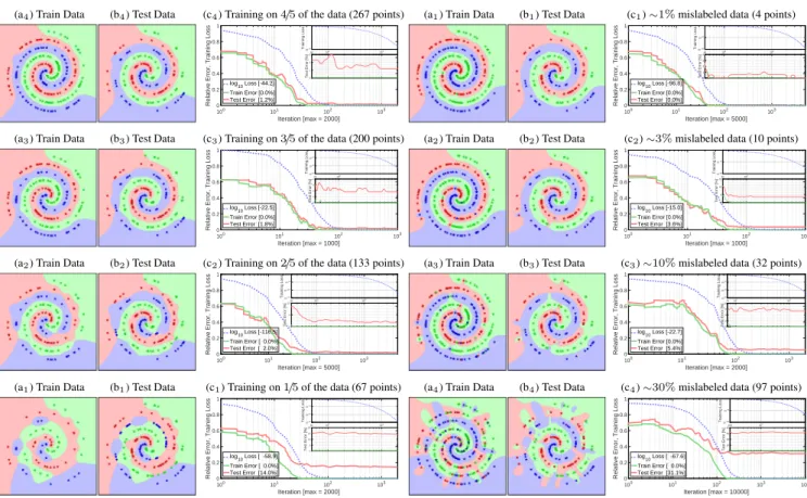
Figure 4. Classification boundaries (a,b), and training curves (c) when a classifier is trained on varying amounts of data. Stars are correctly-classified, circles are misclassified. In all cases, the test error is fairly stable once reaching its minimum.

6.1. Sparse Training Data

In this section of experiments, classifiers were trained using varying amounts of data, from4/5to1/5of the total train-ing set. Fig.4shows the classification boundaries learned by the classifier (ai,bi), and the training curves (ci). In all

cases, the boundaries seem to aptly fit (and notoverfit) the training data (i.e. being satisfied with isolated patches with-outoverzealously trying to connect points of the same class together). This is more rigorously observed from the train-ing curves; the test error does not increase after reachtrain-ing its minimum (for hundreds of iterations).

6.2. Mislabeled Training Data

In this section of experiments, classifiers were trained with varying fractions of mislabeled data; from1%to30%of the training set. Fig.5shows the classification boundaries (ai,bi) and the training curves (ci). All classifiers seem to

degenerate gracefully, isolating rogue points and otherwise maintaining smooth boundaries. Even the classifier trained on30%mislabeled data (which we would consider to be unreasonably noisy) is able to maintain smooth boundaries.

(a1) Train Data (b1) Test Data (c1)∼1%mislabeled data (4 points)

100 ₁₀1 ₁₀2 ₁₀3 Iteration [max = 5000] 0 0.2 0.4 0.6 0.8 1

log 10 Loss [-96.8] Train Error [0.0%] Test Error [0.0%] 10-100 10-50 Training Loss 40 102 103 0 1 2 3 4 Test Error [%]

100 ₁₀1 ₁₀2 ₁₀3 Iteration [max = 1000] 0 0.2 0.4 0.6 0.8 1

log10 Loss [-15.0] Train Error [0.0%] Test Error [3.6%] 10-20 10-10 Training Loss 40 102 0 5 10 15 Test Error [%]

100 ₁₀1 ₁₀2 ₁₀3 Iteration [max = 2000] 0 0.2 0.4 0.6 0.8 1

100 ₁₀1 ₁₀2 ₁₀3 ₁₀4 Iteration [max = 10000] 0 0.2 0.4 0.6 0.8 1

log 10 Loss [ -67.6] Train Error [ 0.0%] Test Error [31.1%] 10-100 10-50 Training Loss 200 103 0 10 20 30 40 Test Error [%]

Figure 5. Classification boundaries (a,b), and training curves (c) when a classifier is trained on varying fractions of mislabeled data. In all cases, the test error is fairly stable once reaching its

mini-mum. Even with30%mislabeled data, the classification

bound-aries are reasonable given the training labels.

In all cases, the training curves still show that the test error is fairly stable once reaching its minimum value. Moreover, test errors approximately equal the fraction of mislabeled data, further validating the generalization of our method. 6.3. Real Data

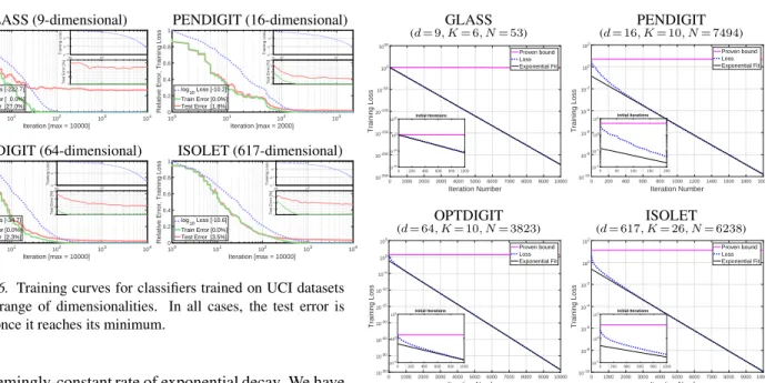
Although the above observations are promising, they could result from the fact that the synthetic datasets are 2-dimensional. In order to rule out this possibility, we performed similar experiments on several UCI datasets

(Bache & Lichman, 2013) of varying input

dimensionali-ties (from 9 to 617). From the training curves in Fig. 6, we observe that once the test errors saturate, they no longer increase, even after hundreds of iterations.

In Fig.7, we plot the training losses on a log-scaled y-axis. The linear trend signifies an exponential decrease in loss per iteration. Our proven bound predicts a much slower (ex-ponential) rate than the actual trend observed during train-ing. Note that within the initial∼10%of the iterations, the loss drops at an even faster rate, after which it settles down

(7)

GLASS (9-dimensional) PENDIGIT (16-dimensional) 100 ₁₀1 ₁₀2 ₁₀3 ₁₀4 Iteration [max = 10000] 0 0.2 0.4 0.6 0.8 1

log10 Loss [-222.7] Train Error [ 0.0%] Test Error [27.0%] 10-300 10-200 10-100 Training Loss 200 103 0 25 30 Test Error [%]~ ~ ~ 100 ₁₀1 ₁₀2 ₁₀3 Iteration [max = 2000] 0 0.2 0.4 0.6 0.8 1

OPTDIGIT (64-dimensional) ISOLET (617-dimensional)

100 ₁₀1 ₁₀2 ₁₀3 ₁₀4 Iteration [max = 10000] 0 0.2 0.4 0.6 0.8 1

log10 Loss [-34.7] Train Error [0.0%] Test Error [2.3%] 10-40 10-20 Training Loss 100 103 0 2 4 6 Test Error [%] 100 ₁₀1 ₁₀2 ₁₀3 ₁₀4 Iteration [max = 10000] 0 0.2 0.4 0.6 0.8 1

Figure 6. Training curves for classifiers trained on UCI datasets with a range of dimensionalities. In all cases, the test error is stable once it reaches its minimum.

to a seemingly-constant rate of exponential decay. We have not yet determined the characteristics (i.e. the theoretically justified rates) of these observed trends, and relegate this endeavor to future work.

7. Comparison with Other Methods

In Sec. 5 we proved that our framework adheres to the-oretical guarantees, and in Sec. 6 above, we showed that it has promising empirical properties. In this sec-tion, we compete against several state-of-the-art boost-ing baselines. Specifically, we compared 1-vs-All Ad-aBoost and AdAd-aBoost.MH (Schapire & Singer, 1999), AdaBoost.ECC (Dietterich & Bakiri, 1995), Struct-Boost

(Shen et al.,2014), CW-Boost (Shen & Hao,2011),

AOSO-LogitBoost (Sun et al.,2011), REBEL (Appel et al.,2016) using shallow decision trees, REBEL using only 1-point (isolating) similarities, and our full framework, REBEL us-ing 2-point localized similarities.

Based on the same experimental setup as in (Shen et al.,

2014;Appel et al.,2016), competing methods are trained

to a maximum of 200 decision stumps. For each dataset, five random splits are generated, with50%of the samples for training,25%for validation (i.e. for setting hyperparam-eters where needed), and the remaining25%for testing. REBEL using localized similarities is the most accurate method on five of the six datasets tested. In the Vowel dataset, it achieves almost half of the error as the next best method. Note that although our framework uses REBEL as its boosting method, the localized similarities add an extra edge, beating REBEL with decision trees in all runs. Further, when limited to only using 1-point (i.e. isolating) localized similarities, the performance is extremely poor, validating the need for 2-point localized similarities as pre-scribed in Sec.5.2. Overall, these results demonstrate the

GLASS PENDIGIT (d= 9, K= 6, N= 53) (d= 16, K= 10, N= 7494) 0 100020003000 40005000 600070008000 900010000 Iteration Number 10-250 10-200 10-150 10-100 10-50 100 1050 Training Loss Proven bound Loss Exponential Fit 0 200 400 600 8001000 10-40 10-20 100 1020 Initial Iterations 0 200 400 600 800 1000 12001400 16001800 2000 Iteration Number 10-10 10-8 10-6 10-4 10-2 100 102 Training Loss Proven bound Loss Exponential Fit 0 50 100 150 200 10-2 10-1 100 101 Initial Iterations OPTDIGIT ISOLET (d= 64, K= 10, N= 3823) (d= 617, K= 26, N= 6238) 0 10002000 30004000 50006000 70008000 900010000 Iteration Number 10-35 10-30 10-25 10-20 10-15 10-10 10-5 100 105 Training Loss Proven bound Loss Exponential Fit 0 200 400 600 8001000 10-5 100 105 Initial Iterations 0 1000 20003000 40005000 60007000 8000900010000 Iteration Number 10-10 10-8 10-6 10-4 10-2 100 102 Training Loss Proven bound Loss Exponential Fit 0 200 400 600 8001000 10-2 100 102 Initial Iterations

Figure 7. Training losses for classifiers trained on UCI datasets. The linear trend (visualized using a log-scaled y-axis) signifies an exponential decrease in loss, albeit at a much faster rate than established by our proven bound.

GLASS VOWEL LANDSAT MNIST PENDIGITS SEGMENT

0 10 20 30 40 Percent Error 31.732.332.735.835.434.230.435.927.4* 21.118.820.617.522.420.617.462.39.5* 15.112.712.812.111.115.410.752.310.6* 11.013.415.812.59.3*12.510.587.19.3* 7.17.4 8.46.9 2.5 12.8 3.2 32.81.2* 7.7 3.72.92.92.5* 5.6 4.6 69.7 3.3 [001] Ada 1vsAll [000] Ada.MH [010] Ada.ECC [020] Struct-Boost [211] CW-Boost [000] A0S0-Logit [032] RBL-Stump [000] RBL-Iso.Sim [500] RBL-Loc.Sim

Figure 8. Test errors of various state-of-the-art and baseline classification methods on MNIST and several UCI datasets. REBEL using localized similarities (shown in yellow) is the best-performing method on all but one of the datasets shown. When constrained to use only 1-point (isolating) similarities (shown in red), the resulting classifier is completely inadequate.

ability of our framework to produce easily interpretable classifiers that are also empirically proficient.

7.1. Comparison with Neural Networks and SVMs Complex neural networks are able to achieve remarkable performance on large datasets, but they require an amount of training data proportional to their complexity. In the regime of small to medium amounts of data (within which UCI and MNIST datasets belong, i.e. 10< N <106

train-ing samples), such networks cannot be too complex. Ac-cordingly, in Fig.9, we compare our method against fully-connected neural networks.

(8)

53 ₅₂₈

38234435559462387494 ₁₆₀₀₀ _4350060000 Number of Training Samples (N)

0.03 0.1 0.3 1 3 10 30 100

Average Test Error [%]

G G G S S S V V V P P P L L L A A A O O O I I I M M M C C C [2/10] NN [2/10] SVM [8/10] Ours GLASS SHUTTLE VOWEL PENDIGIT LETTER LANDSAT OPTDIGIT ISOLET MNIST CUB200 G S V P L A O I M C Method Dataset

Figure 9. Comparison of our method versus Neural Networks and Support Vector Machines on ten datasets of varying sizes and dif-ficulties. Our method is the most accurate on almost all datasets.

Four neural networks were implemented, each having one of the following architectures: [d−4d−K],[d−4K−K],

[d−2d−d−K],[d−4K−2K−K], wheredis the number of input dimensions andKis the number of output classes. Only the one with the best test error is shown in the plot. A multi-class SVM (Chang & Lin,2011) was validated using a5×6parameter sweep forCandγ. Our method was run until the training loss fell below1/N. Overall, REBEL us-ing localized similarities achieves the best results on eight of the ten datasets, decisively marking it as the method of choice for this range of data.

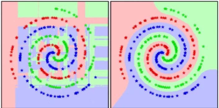
8. Discussion

In Sec.6, we observed that our classifiers tend to smoothen the decision boundaries in the iterations beyond zero train-ing error. In Fig.10, we see that this is not the case with the typically-used axis-aligned decision stumps. Why does this happen with our framework?

Figure 10. The contrasted difference between overtraining using (a) classical decision stumps and (b) localized similarities. (a) leads to massive overfitting of the training data, whereas (b) leads to smoothening of the decision boundaries.

Firstly, we note that the largest-margin boundary between two points is the hyperplane that bisects them. Every two-point localized similarity acts as such a bisector. There-fore, it is not surprising that with only a pool of localized similarities, a classifier should have what it needs to place good boundaries. Further, not all pairs need to be separated (since many neighboring points belong to the same class); hence, only a small subset of the∼N2

possible learners will ever need to be selected.

Secondly, we note that if some point (either an outlier or an unfortunately-placed point) continues to increase in weight until it can no-longer be ignored, it can simply be isolated and individually dealt with using a one-point localized sim-ilarity, there is no need to combine it with other “innocent-bystander” points. This phenomenon is observed in the mis-labeled training experiments in Sec.6.2.

Together, the two types of localized similarities comple-ment each other. With the guarantee that every step reduces the loss, each iteration focuses on either further smoothen-ing out an existsmoothen-ing boundary, or reducsmoothen-ing the weight of a single unfit point.

9. Conclusions

We have presented a novel framework for multi-class boost-ing that makes use of a simple family of weak learners called localized similarities. Each of these learners has a clearly understandable functionality; a test of similarity be-tween a query point and some pre-defined samples. We have proven that the framework adheres to theoretical guarantees: the training loss is minimized at an exponen-tial rate, and since the loss upper-bounds the training error (which can only assume discrete values), our framework is therefore able to achieve maximal accuracy on any dataset. We further explored some of the empirical properties of our framework, noting that the combination of localized similarities and guaranteed loss reduction tend to lead to a non-overfitting regime, in which the classifier focuses on smoothing-out its decision boundaries. Finally, we com-pare our method against several state-of-the-art methods, outperforming all of the methods in most of the datasets. Altogether, we believe that we have achieved our goal of presenting a simple multi-class boosting framework with theoretical guarantees and empirical proficiency.

Acknowledgements

The authors would like to thank anonymous reviewers for their feedback and Google Inc. and the Office of Naval Research MURI N00014-10-1-0933 for funding this work.

(9)

References

Allwein, E. L., Schapire, R. E., and Singer, Y. Reducing multiclass to binary: a unifying approach for margin clas-sifiers. JMLR, 2001.

Appel, R., Burgos-Artizzu, X. P., and Perona, P. Improved multi-class cost-sensitive boosting via estimation of the minimum-risk class. arXiv, (1607.03547), 2016.

Bache, K. and Lichman, M. UCI machine

learning repository (uc irvine), 2013. URL

http://archive.ics.uci.edu/ml.

Chang, C. and Lin, C. LIBSVM: A library for support vec-tor machines. Transactions on Intelligent Systems and Technology, 2011.

Dietterich, T. G. and Bakiri, G. Solving multiclass learn-ing problems via error-correctlearn-ing output codes. arXiv, (9501101), 1995.

Freund, Y. Boosting a weak learning algorithm by majority.

Information and Computation, 1995.

Freund, Y. and Schapire, R. E. Experiments with a new boosting algorithm. InMachine Learning International Workshop, 1996.

LeCun, Y., Bengio, Y., and Hinton, G. E. Deep learning.

Nature Research, 2015.

Li, L. Multiclass boosting with repartitioning. In ICML, 2006.

Mukherjee, I. and Schapire, R. E. A theory of multiclass boosting. InNIPS, 2010.

Saberian, M. and Vasconcelos, N. Multiclass boosting: Theory and algorithms. InNIPS, 2011.

Schapire, R. E. The strength of weak learnability.Machine Learning, 1990.

Schapire, R. E. and Singer, Y. Improved boosting algo-rithms using confidence-rated predictions. InConference on Computational Learning Theory, 1999.

Shen, C. and Hao, Z. A direct formulation for totally-corrective multi-class boosting. InCVPR, 2011.

Shen, G., Lin, G., and van den Hengel, A. Structboost: Boosting methods for predicting structured output vari-ables.PAMI, 2014.

Sun, P., Reid, M. D., and Zhou, J. Aoso-logitboost: Adaptive one-vs-one logitboost for multi-class problem.

arXiv, (1110.3907), 2011.

Sun, Y., Todorovic, S., Li, J., and Wu, D. Unifying the error-correcting and output-code adaboost within the margin framework. InICML, 2005.

Yu, F., Zhang, Y., Song, S., Seff, A., and Xiao, J. LSUN: construction of a large-scale image dataset using deep learning with humans in the loop. arXiv, (1506.03365), 2015.

Zhu, J., Zou, H., Rosset, S., and Hastie, T. Multi-class adaboost.Statistics and its Interface, 2009.