Wavelet Transform Based Methods for Fault Detection and Diagnosis of HVDC Transmission Systems

University of Wisconsin Milwaukee

UWM Digital Commons

Theses and Dissertations

May 2019

Wavelet Transform Based Methods for Fault

Detection and Diagnosis of HVDC Transmission

Systems

Zhongxuan Li

University of Wisconsin-Milwaukee

Follow this and additional works at:

https://dc.uwm.edu/etd

Part of the

Electrical and Electronics Commons

This Thesis is brought to you for free and open access by UWM Digital Commons. It has been accepted for inclusion in Theses and Dissertations by an authorized administrator of UWM Digital Commons. For more information, please [email protected].

Recommended Citation

Li, Zhongxuan, "Wavelet Transform Based Methods for Fault Detection and Diagnosis of HVDC Transmission Systems" (2019).

Theses and Dissertations. 2094. https://dc.uwm.edu/etd/2094

WAVELET TRANSFORM BASED METHODS FOR FAULT DETECTION AND DIAGNOSIS OF HVDC TRANSMISSION SYSTEMS

by Zhongxuan Li

A Thesis Submitted in Partial Fulfillment of the Requirements for the Degree of

Master of Science in Engineering

at

The University of Wisconsin-Milwaukee May 2019

ii ABSTRACT

WAVELET TRANSFORM BASED METHODS FOR FAULT DETECTION AND DIAGNOSIS OF HVDC TRANSMISSION SYSTEMS

by Zhonxguan Li

The University of Wisconsin-Milwaukee, 2019 Under the Supervision of Professor Lingfeng Wang

High-voltage direct current (HVDC) is a key enabler in power system. HVDC offers a most efficient means of transmitting large amount of power. Applications of HVDC can improve the operation security, reliability performance and economy of power systems. Due to factors inside and outside the HVDC system, the system will experience various faults, which have infected HVDC system. VSC-HVDC is a HVDC transmission based on IGBT and PWM. VSC-HVDC direct current transmission has broad application prospects in new energy grid-connected and grid-grid-connected transformation. In this research, aiming at the fault diagnosis of VSC-HVDC, the fault diagnosis and fault detection are studied.

In this research, a VSC-HVDC was simulated in MATLAB Simulink, and an adjusted HVDC model was built. The models were applied to simulate the basic operation of VSC-HVDC and main faults on AC and DC side in the VSC-VSC-HVDC system. Take line current on AC or DC side as input data, the result data after wavelet processing was applied in HVDC faults diagnosis. To verify the function of fault detection, DC faults at different locations were set in the adjusted model. Wavelet entropy was applied in fault diagnosis and detection to gather accurate results.

iii HVDC fault diagnosis and detection.

iv

TABLE OF CONTENTS

LIST OF FIGURES ... vi

LIST OF TABLES ... viii

Chapter 1 Introduction ... 1

1.1 Background ... 1

1.2 Research motivations and objectives... 3

1.3 Research contributions and developments ... 4

1.4 Outline of the thesis ... 5

Chapter 2 Literature review ... 8

2.1 General classification of HVDC system ... 8

2.2 HVDC system configurations ... 14

2.3 Fault diagnosis and detection technology ... 17

Chapter 3 Wavelet transform theory ... 22

3.1 Wavelet transform ... 22

3.2 Comparison between Fourier transform (FT) and Wavelet transform (WT) ... 23

3.3 Wavelet entropy ... 25

Chapter 4 VSC-HVDC simulation ... 27

4.1 VSC-HVDC simulation ... 27

v

Chapter 5 Faults diagnosis using wavelet transform ... 40

5.1 Faults diagnosis in HVDC using Haar wavelet ... 40

5.2 Faults diagnosis in HVDC using Daubechies wavelet analysis ... 45

5.3 Conclusion ... 50

Chapter 6 Fault detection using wavelet transform ... 51

6.1 Simulation model of fault detection in HVDC system ... 51

6.2 Equivalence test of the adjusted simulation model ... 52

6.3 Fault detection using wavelet transform in VSC-HVDC DCLG fault ... 53

6.4 Fault detection using wavelet transform in VSC-HVDC DC LL fault ... 57

Chapter 7 Comparison between wavelet method and particle filter method ... 61

7.1 Introduction ... 61

7.2 Fault analysis using PF ... 62

7.3 Conclusion ... 63

Chapter 8 Conclusion and future work ... 65

vi

LIST OF FIGURES

Fig 1.1 Growth of HVDC Transformer Capacity (MVA)………1

Fig 1.2 Growth of Transmission Line Length (ckt.km) ………2

Fig 2.1 The 12-pulse LCC–HVDC system………9

Fig 2.2 Topologies of the a) 2-level VSC b) 3-level T-type VSC c) 3-level NP………12

Fig 2.3 The structure of the modular multilevel converter………13

Fig 2.4 The curve configuration of sub modular and status of MMC………14

Fig 2.5 Monopolar HVDC system………15

Fig 2.6 Bipolar HVDC system………16

Fig 2.7 Back-to-Back HVDC system………16

Fig 2.8 Multi-terminal HVDC system………17

Fig 2.9 Flowchart of fault diagnosis of an MMC-HVDC………18

Fig 2.10 DC ling to ground fault………19

Fig 2.10 Fig 2.10 DC ling to line fault………20

Fig 3.1 FT of signals with same frequency………24

Fig 3.2 Wavelet tree………25

Fig 4.1 VSC-Based HVDC Transmission Link 200MVA (+/-100kV)………27

Fig 4.2 Signals from VSC-HVDC………28

Fig 4.3 Signals from VSC-HVDC (LG)………30

Fig 4.4 Signals from VSC-HVDC (LLG)………31

Fig 4.5 Signals from VSC-HVDC (LLLG) ………32

Fig 4.6 Signals from VSC-HVDC (LL) ………34

Fig 4.7 Signals from VSC-HVDC (LLL) ………35

Fig 4.8 Signals from VSC-HVDC (DCLG) ………37

Fig 4.9 Signals from VSC-HVDC (DCLL) ………37

Fig 5.1 the Haar wavelet ………40

Fig 5.2 11th wavelet coefficients of Ia for ACLG………41

Fig 5.3 11th wavelet coefficients of Ia for ACLLG………41

Fig 5.4 11th wavelet coefficients of Ia for ACLLLG………42

Fig 5.5 11th wavelet coefficients of Ia for ACLL………42

Fig 5.6 11th wavelet coefficients of Ia for ACLLL………43

vii

Fig 5.8 11th wavelet coefficients of Ia for DCLL………44

Fig 5.9 Daubechies 4 tap wavelet………45

Fig 5.10 9th wavelet coefficients of Idc for ACLG………45

Fig 5.11 9th wavelet coefficients of Idc for ACLLG………46

Fig 5.12 9th wavelet coefficients of Idc for ACLLLG………46

Fig 5.13 9th wavelet coefficients of Idc for ACLL………47

Fig 5.14 9th wavelet coefficients of Idc for ACLLL………47

Fig 5.15 9th wavelet coefficients of Idc for DCLG………48

Fig 5.16 9th wavelet coefficients of Idc for DCLL………48

Fig 6.1 Adjusted VSC-HVDC fault simulation model………49

Fig 6.2 The DC current of adjusted model and original model………51

Fig 6.3 coef. of 5th db4 wavelet transform of DC line current (line to ground-5km) …53 Fig 6.4 coef. of 5th db4 wavelet transform of DC line current (line to ground-15km) 53 Fig 6.5 coef. of 5th db4 wavelet transform of DC line current (line to ground-25km) 54 Fig 6.6 coef. of 5th db4 wavelet transform of DC line current (line to ground-35km) 54 Fig 6.7 coef. of 5th db4 wavelet transform of DC line current (line to ground-45km) 54 Fig 6.8 coef. of 5th db4 wavelet transform of DC line current (line to ground-55km) 55 Fig 6.9 coef. of 5th db4 wavelet transform of DC line current (line to ground) ………55

Fig 6.10 coef. of 5th db4 wavelet transform of DC line current (line to line-15km) …57 Fig 6.11 coef. of 5th db4 wavelet transform of DC line current (line to line -35km) …57 Fig 6.12 coef. of 5th db4 wavelet transform of DC line current (line to line -65km) …58 Fig 6.13 coef. of 5th db4 wavelet transform of DC line current (line to line) …………58

viii

LIST OF TABLES

Table 2.1 Table 2.1 Pros and cons of LCC-HVDC and VSC-HVDC………9

Table 5.1 wavelet entropy………44

Table 5.2 Wavelet entropy………49

Table 6.1 VSC-HVDC DC line to ground fault locations………48

Table 6.2 VSC-HVDC DC line to line fault locations………48 Table 6.3 The absolute value of coef. of the DC line current under faults with different locations o n t h e t r a n s m i s s i o n l i n e … … … 5 3 Table 6.4 The wavelet entropy of 5th _{db4 wavelet of the DC line current under faults with} d i f f e r e n t l o c a t i o n . … … … 5 3 Table 6.5 The absolute value of coef. of the DC line current under faults with different locations o n t h e t r a n s m i s s i o n l i n e … … … 5 5 Table 6.6 The wavelet entropy of 5th _{db4 wavelet of the DC line current under faults with} d i f f e r e n t l o c a t i o n . … … … 5 6

ix

ACKNOWLEDGEMENTS

During the last nine months as a M.S. student in the University of Wisconsin-Milwaukee, many people have helped me in the aspect of academic and culture, without their help I could never complete this thesis. I wish to acknowledge them with my sincere gratitude.

First, I am grateful to my advisor, Dr. Lingfeng Wang, for the great support and encouragement for my M.S study and experiences in UWM. When I first studied in UWM, he guided me into the right direction. His continuous guidance and patience encouraged me to keep digging deeper in academics. Without his instruction I could not have had the accomplishments today.

Special thanks to my thesis committee: Dr. Yi Hu and Dr. Zeyun Yu for their time from their busy schedule. Their advice guides me to further improve thesis.

I shall extend my thanks to Dr. Zhaoxi Liu for all his kindness and help. Without his academic guidance I would make mistakes in research. Also thanks go to my labmates for their advices on my research and the friends from CQU for their support in research.

This work was supported in part by the National Science Foundation Industry/University Cooperative Research Center on Grid-connected Advanced Power Electronic Systems (GRAPES).

1

Chapter 1 Introduction

1.1 Background

When facing the increasing demand of electricity, higher requirements for reliable operation of power systems is needed. HVDC technology is important in the trend of increasingly interconnecting of AC grids and the integration of renewable energy.[1]

The world's earliest HVDC transmission system was built 65 years ago. From there worldwide HVDC transmission capacity growth rapidly. The transformer capacity grew from 3000MVA to 7500MVA (increased by more than 100 per cent) between 2016 and 2017. The growth of 800kV HVDC was greater, which reached 7820 MVA at this period [2].

Fig 2.1 Growth of HVDC Transformer Capacity (MVA) [2] 0

5000 10000 15000

800kV HVDC 500kV HVDC

Growth of Transformer Capacity(MVA)

2

Fig 1.2 Growth of Transmission Line Length (ckt.km) [2]

AC transmission is the preferred system in electrical transmission area for since the electricity became the main source of energy in human society. However, AC transmission system does exist limitations when applied in high voltage area, for instance, the transmission length and the transmission capacity limitations. The Frequency conversion between AC systems with different frequency remain a uneconomical solution. Main applications of the HVDC is as a connection between two AC systems of different frequencies.[3]

As an important part in power transmission system, when operated in long distance, the point-to-point HVDC system has less investment cost and loss than the traditional system[4] Although the cost of the high-voltage DC conversion equipment in the terminal station in the HVDC system is relatively high, the construction cost of total line in HVDC on DC side is lower.[5] The potential for long-distance transmission exists. Using HVDC systems in switchgear increases system stability and improves the power quality of the system. For environmental benefits, compared with the AC transmission system, the HVDC system does not have an induced electromagnetic field

0 5000 10000

800kV HVDC 500kV HVDC

Growth of Transmission Line

Length(ckt.km)

3

generated by the commutation during transmission, and there is no skin effect. The use of cables in HVDC systems reduces losses during transmission and has negligible impact on the surroundings.[6]

1.2 Research motivations and objectives

HVDC has gradually replaced AC systems in long-distance transmission. The efficiency of HVDC is increasing and the system is more complex. Due to factors inside and outside the HVDC system, the system will experience various faults, which have horrible inflect on HVDC system, causing a losing of features.

The aim of HVDC faults analysis is to complete the diagnose various HVDC faults fast and accurately, provide necessary guidance for the operation of the system, improve the reliability, safety and effectiveness of system operation, reduce the fault loss to a minimum level, and through fault analysis, provide data and information for system structure modification and optimization design. In a HVDC system, HVDC line faults on AC and DC sides are common.

Some serious failure also causes damage to the equipment and economic losses. In severe cases, HVDC faults cause casualties and serious social impact. Therefore, the fast and accurate HVDC fault analyzing technologies are necessary to the HVDC reliable operation. Therefore, HVDC fault analysis technology including faults classification and faults detection is needed.

Signal processing techniques is considered as a reliable method in HVDC faults analysis. Currently the mean methods used in HVDC faults analysis include wavelet

4

transform, artificial neural network, fuzzy logic and etc. Among these methods, wavelet transform is a very effective method for fault diagnosis. Considering signals with that multiple frequencies are generated when a HVDC fault occurs, applying wavelet, as a signal processing method that can analyze both time domain information and frequency domain information, in HVDC faults analysis is a correct choose. In this research wavelet is used for fault analysis in VSC-HVDC system, and it is proved that wavelet has very great results in the diagnosis of faults, whichmake it possible to use wavelet transform for fault analysis.

1.3 Research contributions and developments

According to the objectives mentioned above, this research has led to the following contributions and developments:

1) In Chapter2 literature review, the general classification of HVDC system, HVDC system configurations and fault diagnosis and detection technology are introduced. 2) In this research wavelet transform is used in VSC-HVDC faults analysis, the result shows the consequent of wavelet transform in HVDC faults analysis is good. Wavelet transform can judge the HVDC faults types and detect the location fast ad accurately.

3) AC faults in VSC-HVDC has been detected successfully using both haar wavelet and db4 wavelet.

4) DC faults in VSC-HVDC has been detected successfully using both haar wavelet and db4 wavelet.

5

5) Using db4 wavelet at 5th _{level to detection DC line to line faults at different location} on DC line successfully.

6) Using db4 wavelet at 5th _{level to detection DC line to ground faults at different} location on DC line successfully.

7) For gathering more accurate results, wavelet entropy is considered in faults classification and detection.

8) Compared between wavelet based method and PF based method in HVDC faults analysis, the results shows the advantages of wavelet transform in HVDC faults analysis.

1.4 Outline of the thesis

1) Introduction

Background of HVDC in power system, the motivations, contributions and developments, HVDC model and measurements will be discussed.

2) Literature review

General aspects of HVDC is introduced, including VSC-HVDC, LCC-HVDC and MMC-HVDC. Fault analysis in HVDC and summary of HVDC fault diagnosis methods will be discussed.

3) Wavelet transform theory

In this chapter, the theory of wavelet transform will be discussed, including the definition of wavelet transform, DWT, CWT, wavelet entropy will be discussed, which is applied in HVDC fault diagnosis and detection in Chapter 5 and Chapter 6.

6 4) VSC-HVDC simulation

Simulation of VSC-HVDC in Simulink will be discussed. The simulation includes normal situation and HVDC under different kinds of faults (5 kinds of AC fault and 3 kinds of DC faults)

5) Faults diagnosis in HVDC using wavelet transform

The VSC-HVDC simulation model is applied in simulate different kind of HVDC faults on AC and DC side, including AC short circuit fault, AC grounding fault, DC line to line fault and DC line to ground fault. Transmission line current is applied which are input data in wavelet transform.

Results of WT under different HVDC faults will be used to explain how WT works in faults diagnosis in HVDC.

6) Fault (different locations) detection in HVDC using wavelet transform

An adjusted model of VSC-HVDC is introduced, the model is applied to simulate HVDC fault at different locations on DC transmission lines. To judge whether the model is suitable for the real HVDC system, an equivalence test of the adjusted simulation model is considered, the result illustrates the model work well in simulating the HVDC fault at different locations.

The results of WT under faults in different locations in HVDC will be used to explain how WT works in faults detection in HVDC.

7) Comparison between wavelet method and particle filter method

In this chapter, fault diagnosis using particle filter will be discussed and compared with wavelet transform.

7

The result show that although PF can achieve the classification on some HVDC faults, PF based method still perform not as good as wavelet-based method.

8

Chapter 2 Literature review

To face the increasing power transmission, HVDC system is a reliable electronic technology designed for decreasing the transmission losses and increasing the efficiency in long distance power transmission. 60 years have passed since the first HVDC system was built, HVDC systems have a great improvement. As an alternative method of power transmission in a long distance, HVDC system has some negligible advantages compared with traditional system.

In a HVDC the converter has high influences on reliable operation and rated power of HVDC systems [8]. The HVDC currently used in the field of power transmission mainly includes LCC-HVDC, VSC-HVDC and MMC-HVDC. Each of these technologies has its application and unique advantages.

2.1 General classification of HVDC system

A. LCC HVDC

The thyristor-based Line Commutated Converter (LCC) was developed at 1970s[9]. The low loss of 0.7% per converter make LCC a good choice for HVDC system[9]. However, LCC is not perfect, there still exists some drawbacks that can’t be ignored. One main disadvantage of LCC system is that both requires reactive power consumptions. It is also needed to install an AC voltage source at every ending to achieve with commutation which increased the cost of system design and construction. Besides, in the LCC converter the voltage is leading the current, which makes the

9

converters consume reactive power[10]. In the LCC, the converters absorb reactive power which value equals 50% to 60% of active power. All those drawbacks all make the LCC need to improve to make the demand of power transmission using HVDC system.

An LCC-HVDC is shown in fig 2.1.

Fig 2.1 The 12-pulse LCC–HVDC system [12]

B. VSC-HVDC

With the continuous expansion of the use of renewable energy [13], inherent dispersion, smallness, and long distance from the load center makes the use of AC transmission technology or traditional current source converter type DC transmission technology networking uneconomical. Therefore, it is necessary to apply a more economical and environmentally friendly transmission means to solve the problems from the traditional HVDC system. Researches on power electronics and control technology, IGBT, IGCT and other components are need to form a voltage source converter (VSC) [15]. Since the late 1990s, foreign companies represented by ABB have developed HVDC Light technology [16]. It uses a voltage source converter based on a turn-off device and PWM technology for DC power[17]. Compared to LCC, the

10

semiconductor used by VSC can transfer current in any direction. And VSC stores energy capacitively. To get a more specific comparison, the table 2.1 shows the pros and cons of LCC and VSC. [18].

Table 2.1 Pros and cons of LCC-HVDC and VSC-HVDC

At present, 2 level VSC and 3 level VSC now are applied as voltage source converters in flexible DC transmission projects. Fig 2.2 shows the topology of 2 level VSC, 3 level T-type VSC and 3-level NPC VSC.

In 2 level VSC, two bridge arms per phase. IGBT and diode are applied in the three phases. The amount of series is controlled by inverter voltage level, and the flow capacity and compressive strength of the power electronic switching device. The IGBTs on 3 phases are turned on in turn, output DC voltage ⁄2 and − ⁄2, and

LCC-HVDC VSC-HVDC

Strong AC systems is needed Can operated in a weak AC system

Harmonic distortion generation AC & DC harmonic filters are needed

Little harmonic generation

Bad in reactive power control Better than LCC-HVDC

Higher losses Less losses

Higher cost Lower cost

Change polarity of the converters to reverse power

Chang current flow direction to reverse power

11

approximates a sine wave by PWM. Two-level VSC has certain defects in large-capacity and high-voltage transmission. The main reason is that the voltage and current that the switching device can withstand is limited. The voltage can only be increased by increasing the series connection of the switching devices. Excessive series connection will cause it.

The difference between a 3 level VSC and a two-level VSC is that a DC capacitor is shared between the bridge arms, so that a level of 0 V can be output. With the same switching device, the DC voltage of 3 level VSC converter is doubled, contrasted to the 2 level VSC, and voltage level increases. However, since the voltage is still required to directly connect the switching devices, the problem of capacitor voltage equalization and large harmonic content cannot be effectively solved.

12

a) 2-level VSC b) 3-level T-type VSC

c) 3-level NPC

Fig 2.2 Topologies of VSC [19]

C. MMC-HVDC

When the number of VSC output levels is large, the required floating capacitance will increase sharply, which will bring great difficulties to system control and equipment assembly. To face the problem Modular Multilevel Converter (MMC) has received more attention. Compared with VSC-HVDC, MMC-based HVDC (MMC-HVDC) systems have obvious advantages in reducing switching losses, fast faults recovery, capacity upgrades, electromagnetic compatibility, and fault management[20].

The modular multilevel converter (MMC) is shown in fig2.3. There are submodules in every arm and a series reactor instead of switching devices.

13

Fig 2.3 Structure of MMC [23]

Fig 2.4 shows curve configuration of sub modular and status of MMC. MMC adjust the status of the sub modular through T1 and T2 to achieve multiple outputs: 0, Uc and Isolated.

14

Fig 2.4 The curve configuration of sub modular and status of MMC [23] In the MMC inverter circuit, the more sub-modules there are, the output waveform is approximate to the sine wave. Comparing the switching frequency, it can be observed that of the frequency of VSC converter is much bigger than the frequency of MMC converter, and the loss of the converter is also greatly improved. However, as the transmission voltage increases, a large number of modular units are needed, which increases the design and implementation difficulty of the control system.

2.2 HVDC system configurations

To satisfy the effective function, there are several configurations that is identified. When choosing the HVDC configuration, the function and location of the converter station are two main bases of the selection. At present, the main structures include

15

monopolar HVDC system, bipolar HVDC system, back-to-back HVDC system and multi-terminal HVDC system.

A. Monopolar HVDC

A monopolar HVDC system is indicated in Fig 2.5. Unipolar system has a wire that uses the earth or ocean as the return line. Metal lines can also be used when considering harmonic interference or radiation problems. In DC cable applications (such as lightweight HVDC), a return cable is required. Since the corona effect of the negative connection wire is lighter than that of the positive connection wire, the unipolar system usually operates with the negative electrode[26]. The monopolar link is not much in use nowadays.

Fig 2.5 Monopolar HVDC B. Bipolar HVDC

A bipolar system has two wires, one positive wire the negative wire. At each end of the DC side, there are two sets of inverters with the same rating. The tie line between the two sets of inverters is grounded through a short wide electrode line. Since the two poles have the same current under normal conditions, the ground current is zero. Unipolar operation can be employed in the first phase of implementing a bipolar system. Also, in the event of an inverter failure, a metal wire can be temporarily used as a return

16

line through a suitable switch[26]. The bipolar HVDC is indicated in Fig 2.6.

Fig 2.6 Bipolar HVDC C. Back-to-Back HVDC

In modern transmission system, Back-to-Back HVDC is a solution to realize the interconnection of different Grids when power grids and power system aren’t in synchronization with other grid or systems. A Back-to-Back HVDC is indicated in figure 2.7. The Back-to-Back HVDC is mainly used for networking or power transmission between two asynchronous power systems[27]. By using the Back-to-Back HVDC, the system is adjusted to desired frequency. Two systems can be connected without losing stability.

Fig 2.7 Back-to-Back HVDC

D. Multi-terminal HVDC (MTDC)

17

MTDC system[30]. In multi-terminal system, the UDC is revised by one converter and the power flow is determined by the others [31].

Fig 2.8 Multi-terminal HVDC

2.3 Fault diagnosis and detection technology

Any fault occurs in HVDC system will lead to a unique change of parameters which make it possible to use the signals processing technology in faults diagnosis and detection in HVDC system. These changing parameter values carry the information of faults which is the aim of HVDC fault diagnosis and detection. To distinguish fault types and find the location of the fault, two general mechanisms are considered: on the one hand, make a comparison between the actual and theoretical values. When the faults occur, in general a significant deviation will exist between actual and theoretical values. On the other hand, the appearance of HVDC faults will expressed in a certain pattern, therefore in HVDC faults diagnosis, the detection of these patterns is meaningful[32]. Fig. 2.9 shows a flowchart of fault diagnosis of an MMC-HVDC.

18

Fig 2.9 Flowchart of fault diagnosis of an MMC-HVDC [32]

When achieving HVDC fault diagnosis, some step should be followed:

a) Sampling at important locations (HVDC transmission lines, converters, inverters and etc.) of the HVDC system in every sampling period and send the relative signals values (Grid voltage, DC side positive and negative voltage, DC voltage, Three-phase voltage, Three-phase current, grid current arm current, active power, reactive power and etc.) to interface to finish the follow steps.

b) Compare the detection signal value with the reference signal value and contrast signal changes to determine if a particular mode of failure has occurred.

c) Data processing methods may be used to process the detected signals data: filtering, normalize, extraction and etc.

d) Gather the key information which express the types of the faults. In this step plenty of signals processing technologies could be considered (Fourier analysis [33],

19 wavelet analysis[34], ANN[41] and etc.).

The main faults in HVDC system need to be analyzed quickly. Many kinds of faults occur on HVDC system on both DC and AC side.

In HVDC, DC transmission lines are one of the components that the faults occur. The two main types of DC fault in HVDC are grounding fault and short-circuit fault. The abovementioned faults are the most basic faults in HVDC.

2.3.1 Line to ground fault

Research shows that there is no overhead DC line has been installed in any VSC-HVDC and most VSC-VSC-HVDC system is connected through the underground cables[44], which makes the line to ground fault common. In general, reason of the grounding fault is the occurrence of the damaged insulation of the underground cables. When insulation failure causes damage on DC cables, the DC-side capacitor will discharge to generate a large overcurrent.

Fig 2.10 DC line to ground fault 2.3.2 Line to line fault

Compared with grounding fault, line to line fault is a rare fault in HVDC system. Insulation failure between the transmission lines results in line to line fault. When such faults occurs, AC system will three phase short currented at the fault point in DC side.

20

Fig 2.10 Fig 2.10 DC ling to line fault 2.3.3 AC faults

AC faults also occur in HVDC transmission system. Research shows that common AC faults include AC two-line short circuit fault, AC single line grounding faults, three phases short circuit fault. These faults could cause huge damage which are tried to avoid. Therefore, AC faults in HVDC system need to be studied.

Wavelet transform has been widely used in several areas, which is a time domain-frequency domain analysis[45]. Compared with other signal processing technology, wavelet has its unique advantages:

1) The frequency and time axis can be observed simultaneously, with good sensitivity to time under high frequency conditions and good sensitivity to frequency under low frequency conditions.

2) In wavelet theory, you can approximate a function with fewer wavelet coefficients. 3) When the signal is denoised or compressed, there is no significant damage to the

signal.

4) The detailed information is separately saved[46].

The research on wavelet transform in fault diagnosis has proved to be effective. Fast and reliable fault diagnosis is preferred in HVDC system. therefore, wavelet

21

transform is used for fault diagnosis with its unique advantages. In [47], author picks up the key information from vibration signals from a machine which represent that wavelet analysis preforms good in signal processing and extraction. Author in [48] establishes a VSC-HVDC model and wavelet analysis is adopted to pick up the feature of the fault signals. Author in [35] introduces a high speed HVDC fault analysis method based on wavelet technology. In the research, the protection can judge the types of HVDC faults well. Yuhong in [49] study a commutation failure detection method based on wavelet analysis, the result represents that using DWT by Daubechies wavelet function in HVDC fault diagnosis is very effective.

Combining wavelet transform with other data processing methods is also considered to be an effective method for HVDC fault diagnosis. Author in [50] adopts the neural network with wavelet packet in the research of HVDC line fault detection, result indicates that the algorithm can find the location of HVDC transmission line fault accurately. In [51] a HVDC short circuit fault analysis method using wavelet analysis combined with fuzzy system is introduced. To detect faults in a multi-terminals HVDC systems, author in [52] proposes a wavelet-fuzzy logic-based protection algorithm.

22

Chapter 3 Wavelet transform theory

3.1 Wavelet transform

WT is proposed facing the deficiency of traditional data processing method. Wavelet overcomes the shortcomings of Fourier and windowed Fourier transform, and can analyze the local characteristics of time-varying signals. In principle, problems that can be analyzed by Fourier transform is replaced by wavelet transform, which is expressed by the following equation:

, = , (3.1)

When the function ∈ can described as = 0, the

is called mother wavelet.

The commonly used wavelet mother functions are mainly considered as the following:

(1) Classic wavelet: Harr wavelet, Morlet wavelet and Gaussian wavelet.

(2) Orthogonal wavelet: Daubechies wavelet, Symlets wavelet and Coiflets wavelet.

(3) Biorthogonal wavelet

3.1.1 Continues wavelet transform (CWT)

Mathematical definition of continuous wavelet transform of is described as follows:

! ", = #_√$# &' (

23

The daughter wavelet _, is the stretching and translating of a mother wavelet . In the formula, parameter y shows degree of the scaling, and parameter z shows degree of the translation. Parameters x, y, z are continuous variables.

3.1.2 Discrete wavelet transform (DWT)

When performing CWT, if you want to perform calculations on various scales, it will lead to excessive calculation and reduce computational efficiency. To solve this problem, DWT is applied. In DWT, y and z also represent the degree of scaling and translation, the difference is that in DWT sampling of the two key parameters y and z of continuous wavelets is applied, which is generally sampled at base 2.

DWT (Discrete wavelet transform) is defined as: * ! ", ) =_√$ &' (

" = 2+_{, ) = ,2}+_{, ,, - ∈ .} (3.3)

3.2 Comparison between Fourier transform (FT) and Wavelet transform (WT)

FT does not reflect frequency that changes over time, that is, for a certain frequency is detected, when it is generated can’t be determined from Fourier transform. The Fourier transform lacks the local signal analytical ability. It can be observed from Fig3.1.

Facing this drawback, Translation and expansion are a feature of wavelet transform. Therefore, various signals can be analysed in different frequency ranges and different time positions. Through this multi-resolution analysis, a good time sensitivity is obtained in high-frequency signals. Good sensitivity to time and frequency at

24

different frequencies of wavelet solve the disadvantages of FT applications and non-stationary signals. The FT lost the time information of the original signal.

Fig 3.1 FT of signals with same frequency

Equation (3.4) and (3.5) is the definition of FT and WT from where shows the difference between FT and WT[54].

/ =_{√ 0}$ 1 2 +34 _{1 (3.4)}

, = 1 5,6&4 6₅ ( , , ∈ , ≠ 0 (3.5) In (3.5), _5,6 1 is continuous wavelet, translated and scaled from mother wavelet, as shown in (3).

25 3.3 Wavelet entropy

Apply wavelet transform in processing signal, the wavelet transform decomposes the signal into two components Di(x) and Ai(x) at parameter x and i. Di(x) and Ai(x) respectively represent the different frequency parts of the entire signal:

;*<_A : >2 < $ ?, 2 < ?@

< : >0, 2 < $ ?@ B = 1,2,3, ⋯ , F

(3.7)

As the wavelet tree show in Fig 3.2, the previous decomposition is performed by decomposing the signal into components of different frequencies Di(n-1) and Ai(n-1), and then the low frequency component Ai(n-1) is again decomposed into components of different frequencies in next stage, where Ai(n) contains the information missing by the Di(n) after the decomposition of Di(n-1).

G H = *$ H + A$ H = *$ H + J* H + A H K = *$ H + * H +

J*L H + AL H K = ⋯ = ∑ *<<N$ < H + A< H (3.8)

Fig 3.2 Wavelet tree

Define mathematical expectations as the entropy H(X) of the information source: O P = QJR < K = QJ−STU5V<K = − ∑ VW<N$ <STU5V< (3.9)

26

Combining the wavelet with entropy as a reference in HVDC fault diagnosis and detection.

In this research Shannon entropy is applied in classification of HVDC faults and fault detection. The calculation of wavelet Shannon entropy is as follows:

Q+= − ∑ QX <'STUQ<' (3.10) Q<' = |*< | (3.11) After a normal system experiences a fault, the characteristics of the observed signal will change. The Shannon entropy will also change accordingly. This entropy will give the ‘energy information’ of the signal. The Shannon entropy E can be calculated from the equation

Q Y = − ∑ Y+ <log Y< (3.12)

si is the coeff. of details or approximation of signal s after WT, which is perpendicular to the base s. The advantage of using Shannon entropy is, it will store more energy of the waveform. Shannon entropy can be used for a feature pickup and generate characteristic vector.

27

Chapter 4 VSC-HVDC simulation

4.1 VSC-HVDC simulation

A VSC-HVDC simulation is applied as the model. The VSC-HVDC represents a 200 MVA, ±100 kV voltage source converter as the interconnection of a 230 kV (phase to phase), 2000 MVA AC system and another AC system.

Fig 4.1 VSC-HVDC model[55]

In the VSC-HVDC model the signal output includes the following: Vdc - DC side positive and negative voltage

Uabc - Three-phase voltage Iabc - Three-phase current Idc - DC line current

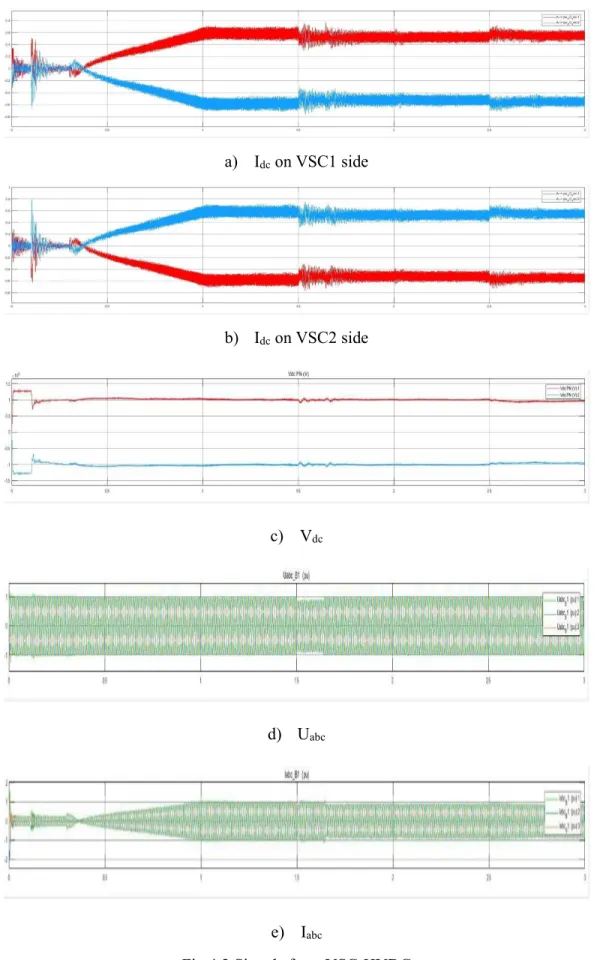
When the VSC-HVDC operates without any failure, the simulation results are indicated as following. The simulation is set 3s.

28 a) Idc on VSC1 side b) Idc on VSC2 side c) Vdc d) Uabc e) Iabc

29 4.2 HVDC faults simulation

In this research faults on system level are considered. Considering the practical reality that if the system experiences a DC cable open circuit fault, the normal operation must be interrupted. Open circuit faults of the DC cable are not considered in this research. Based on this assumption.

4.2.1 AC side faults in VSC-HVDC

In this research, 5 kinds of faults on AC side is considered. The system is under normal condition before 2.0s. When the system experiences a line to ground (LG, LLG, LLLG) fault, the signals fluctuation at the VSC1 side is shown in Fig 4.3. From the time period 1.5 to 1.9 second the normal value of Idc is 0.5 pu. the system experiences a fault at 2 to 2.1s. Idc decreases with significant fluctuations. As for Uabc and Iabc, when the fault occurs, the fault has little effect on Uabc at Bus 1 side, and the voltage of the ground phase reduced to zero. Circuit in ground phase didn’t change, although circuit in other phase has a big fluctuation in bus 2 side. Iabc in bus 1 side gradually decreases as grounding lines increases

A. Grounding fault

If system experiences a single line grounding fault (LG) fault after 2.0s in this simulation, the fault has a significant impact on Idc, Uabc and Iabc. When the fault begins at 2.0s, negative peak value of the Idc reaches 0 pu, and positive peak value of the waveform reaches 0.9 pu.

30

a) Idc on VSC1 side

b) Iabc

c) Uabc

Fig 4.3 Signals from VSC-HVDC (LG)

When the system experiences a double line grounding fault (LLG) after 2.0s in this simulation, the impact of the fault on Idc is the same expect the value. Negative peak value of the Idc reaches -0.3 pu, and positive peak value reaches 0.9 pu.

31

a) Idc on VSC1 side

b) Iabc

c) Uabc

32

When the system experiences a triple line grounding fault (LLLG) after 2.0s in this simulation, the impact of the fault on Idc is the same expect the value. When the fault begins at 2.0s, negative peak value of the Idc reaches -0.5 pu, and positive peak value of the waveform reaches 1.1 pu.

a) Idc on VSC1 side

33 c) Uabc

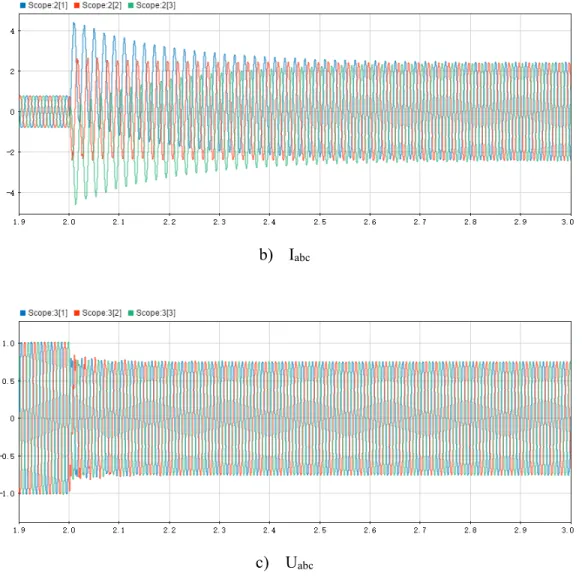
Fig 4.5 Signals from VSC-HVDC (LLLG) B. Two phases short circuit fault (LL)

When this fault occurs between two phases, there is almost no change in value of Udc but fluctuation is obvious. Vdc in both sides increase slightly with fluctuation. Uabc change obvious and Ua and Ub decrease to half and Ia and Ib increased to 2 pu.

34 b) Iabc

c) Uabc

Fig 4.6 Signals from VSC-HVDC (LL) C. Three phases short circuit fault (LLL)

When the system experiences this kind of fault, compared with the two phase grounding fault, Udc has a bigger change, which increased to 1.25 pu. Iabc decreased to 0.2 pu in bus 1 side. Udc decreased to 0 and Iabc has a little increase from to 1.5 pu.

35

a) Idc on VSC1 side

b) Iabc

c) Uabc

36 4.2.2 DC side faults in VSC-HVDC

A. Line to ground fault (DCLG)

From time period 2.0s. The normal value of the three phases current is 1.0 pu. Then the fault occurred at 2 second. During this time period the current increases to 4.0pu with significant fluctuations. During the whole period three phase voltage increases to 1.8 pu with significant fluctuations. Idc reaches 5 pu and decreases to 1pu, after that the Idc increases to 6 pu with significant fluctuations.

a) Idc on VSC1 side

37 c) Uabc

Fig 4.8 Signals from VSC-HVDC (DCLG) B. Line to line fault (DCLL)

The last case studies the DCLL fault. From the time period 2.0s. The normal value of the three phases current is 1.0 pu. Then the fault occurred at 2 second. During this time period the current increases to 4.0pu. Again from 2.4 second onwards current is maintained to 2.0pu as shown in figure. During the whole period three phase voltage decreases to 0.8 pu. Idc has a huge increase when the fault begins at 2.0s which value reaches to 5.5pu, then Idc decreases rapidly to 0.

38 b) Iabc

c) Uabc

Fig 4.9 Signals from VSC-HVDC (DCLL)

Compare with the normal status, the line to ground fault has some influences: For Bus 1 side:

(1) When the occurrence of fault is detected, the positive voltage of DC decreases to 0 and negative voltage increases from -1 pu to -2 pu with a more dramatic fluctuation

(2) there is no difference in P and Q, no matter whether the fault is generated or not, and P and Q fluctuate during the whole fault period.

39

(3) The absolute value of max value of the three-phase voltage is slightly increased to 1.5 pu, the harmonic components in the three-phase voltage are also rich in harmonic components. When the fault occurs, three-phase current reaches 2 pu in process of fault, and distortion is severe.

Bus 2 side:

40

Chapter 5 Faults diagnosis using wavelet transform

5.1 Faults diagnosis in HVDC using Haar wavelet

Haar wavelet the earliest one applied in research. It is seen as a db wavelet. Haar is also called Daubechies1 wavelet. Db1 proposed an orthogonal function system in 1990[56]. The definition of mother wavelet function t is[58]:

t = ^ _ ` _ a 1 , 0 b 1 c1₂ −1, 1_{2 b 1 c 1} 0, T1d2efBY2

This is the simplest orthogonal wavelet[57]:

g t t − n = 0, H = i1, i2, …

Fig 5.1 the Haar wavelet [61]

Take the data of three phases circuit of the fault line as input. The 11th _level coefficients shows a clear distinction.

5.1.1 Haar wavelet analysis under ACLG

In the case a single line grounding fault is stared at 2.0s to 2.1s. From this analysis it is observed that the max value of the approximation reached 1.08 pu and -2.06 pu.

41

Fig 5.2 11th wavelet coefficients of Ia for ACLG 5.1.2 Haar wavelet analysis under ACLLG

In the 2th case a double line grounding fault is occurs at 2.0s to 2.1s. From this analysis it is observed that the max value of the approximation reached 1.33 pu and -1.09 pu..

Fig 5.3 11th wavelet coefficients of Ia for ACLLG 5.1.3 Haar wavelet analysis under ACLLLG

In the 3th case the HVDC system experiences a triple line grounding fault from 2.0s to 2.1s. From this analysis it is observed that the max value of the approximation

42 reached 1.01 pu and -0.7 pu.

Fig 5.4 11th wavelet coefficients of Ia for ACLLLG

5.1.4 Haar wavelet analysis under ACLL

In the 4th case two phases short circuit fault is occurs at 2.0s to 2.1s. From this analysis it is observed that the max value of the approximation reached 0.59 pu and -0.45 pu.

Fig 5.5 11th wavelet coefficients of Ia for ACLL 5.1.5 Haar wavelet analysis under ACLLL

43

2.0s to 2.1s. From this analysis it is observed that the max value of the approximation reached 0.35 pu and -0.7 pu.

Fig 5.6 11th wavelet coefficients of Ia for ACLLL 5.1.6 Haar wavelet analysis under DCLG

In the DC line to ground fault initiated at 2.0s, from this analysis it is observed that the max value of the approximation reached 1.25 pu and -0.72 pu.

Fig 5.7 11th wavelet coefficients of Ia for DCLG 5.1.7 Haar wavelet analysis under DCLL

44

value of the approximation reached 2.52 pu and -0.63 pu.

Fig 5.8 11th wavelet coefficients of Ia for DCLL

When HVDC faults occur, data after Haar wavelet analysis shows different results i. This can be used in HVDC faults detection and classification.

Table 5.1 wavelet entropy

Judging from the appearance, faults can be divided into three categories: AC grounding fault, AC short circuit fault and DC fault.

Fault Entropy AC LG -4.011E+03 LLG -6.183E+03 LLLG -6.574E+03 LL -6.735E+03 LLL -6.563E+03 DC LG -8.922E+03 LL -1.784E+04

45

Judging from entropy, -the entropy of ACLG is 4.01E+03, -the entropy of DCLG is 8.92E+03, the entropy of DCLL is 1.78E+04. the entropy of other faults is about -6.5E+04.

Judging from entropy combined with coefficients, max coef. of ACLLG is about 4 times as much as normal, max coef. of ACLLLG is about 3 times as much as normal situation, max coef. of ACLL is slightly larger than normal, the positive max value of ACLLL is approximately equal to normal situation and absolute value of negative max value is 4 times as much as absolute value of positive max value.

5.2 Faults diagnosis in HVDC using Daubechies wavelet analysis

Meyer wavelet [59], Daubechies wavelet, Mexican Hat wavelet[60] as the main choice are used in many reasreach. In this chapter Daubechie 4 (db4) wavelets is used in wavelet analysis which is found most commonly in power signal analysis. The db4 wavelet will give the transient behavior of fault more accurately. It is effective for the detection of fast and short transient disturbances [61]. The Daubechie, “db4” wavelet function was adopted to perform the wavelet, because it is having larger energy distribution of the decomposition levels [62].

46

Fig 5.9 Daubechies 4 tap wavelet 5.2.1 Db4 wavelet analysis under ACLG

In the first case the HVDC system experiences an AC single line grounding fault from 1.5s to 2s. The corresponding wavelet coefficients of the DC line current in the 9th level is as follow. It indicates the detection capability of wavelet transform.

Fig 5.10 9th wavelet coefficients of Idc for ACLG 5.2.2 Db4 wavelet analysis under ACLLG

In 2nd case a double line grounding fault is occurred at 2.2s, the fault lasted foe 0.2s. The corresponding 9th level wavelet coefficients of DC line current are plotted in

47 Fig. 5.10.

Fig 5.11 9th wavelet coefficients of Idc for ACLLG

5.2.3 Db4 wavelet analysis under ACLLLG

In 3rd case a triple line grounding fault is stared at 2.2s. The corresponding 9th level wavelet coefficients of DC line current are plotted in Fig. 5.11.

Fig 5.12 9th wavelet coefficients of Idc for ACLLLG 5.2.4 Db4 wavelet analysis under ACLL

In next case the system experiences a two phases short circuit fault from 2.2s to 2.4s. The corresponding 9th level wavelet coefficients of DC line current are plotted in

48 Fig. 5.12.

Fig 5.13 9th wavelet coefficients of Idc for ACLL

5.2.5 Db4 wavelet analysis under ACLLL

In next case a ACLLL fault occurred at 2.2s and ended at 2.4s. The corresponding 9th level wavelet coefficients of DC line current are plotted in Fig. 5.13.

Fig 5.14 9th wavelet coefficients of Idc for ACLLL 5.2.6 Db4 wavelet analysis under DCLG

In other case line to ground fault of DC side is initiated at 2.2s to 2.4s. The corresponding 9th level wavelet coefficients of DC line current are plotted in Fig. 5.14.

49

Fig 5.15 9th wavelet coefficients of Idc for DCLG 5.2.7 Db4 wavelet analysis under DCLL

In the last case, the system experiences a DCLL fault from 2.2s to 2.4s. The corresponding 9th level wavelet coefficients of DC line current are indicated in the following figure.

Fig 5.16 9th wavelet coefficients of Idc for DCLL Table 5.2 Wavelet entropy

Fault ACLG ACLLG ACLLLG ACLL

50 5.3 Conclusion

In this research, the classification of both HVDC DC faults on transmission lines and HVDC AC faults at convertor side and invertor side using wavelet transform is achieved.

The results illustrate that the absolute value of wavelet coefficients and entropy differ from each other when system experiences different fault. Based on this result, in HVDC faults diagnosis, wavelet coefficients and entropy could be analyzing conditions.

Fault ACLLL DCLG DCLL Normal

51

Chapter 6 Fault detection using wavelet transform

The detection of the occurrence of faults is not enough to make sure HVDC works normally and efficiently. After classification the HVDC fault using wavelet transform, determining the specific location of the fault is also a necessary aim of fault analysis in HVDC system.

In this chapter, faults simulation model will be adjusted based on the aim of fault detection in HVDC power systems. HVDC DC fault will be set with different parameter to simulate different fault locations in operation of HVDC systems. In this chapter DCLG faults and DCLL faults set at different locations on the DC transmission line will be tested.

6.1 Simulation model of fault detection in HVDC system

Fig 6.1 Adjusted VSC-HVDC fault simulation model

The VSC-HVDC simulation model in Simulink mentioned in Chapter 4 simulate different kind of faults in VSC-HVDC system without the location information. To achieve the simulation with HVDC faults at different location, a adjustment in VSC-HVDC model is adopted. To adjust the location of VSC-HVDC fault in DC transmission lines, 2 separate cables are connected in series instead of the original cable structure. The purpose of setting up two separate cables is to simulate the different location of

52

HVDC fault. Each cable represents the cable on both sides of the fault point. The length of the cable can be adjusted freely and the sum of the length equals 75km which is the length of the cable in the model of Chapter 4. Other parameters are consistent with the origin model.

In this research, 7 different locations of HVDC DCLG fault and 3 different locations of HVDC DCLL fault are set to complete the simulation. Location information are set as following.

Table 6.1 VSC-HVDC DCLG fault locations

Table 6.2 VSC-HVDC DCLL fault locations

6.2 Equivalence test of the adjusted simulation model

This test is set to study whether the adjusted model still can represent the actual operation of HVDC system. Run both the original model and the adjusted model without any HVDC fault. And IDC data is used to compare to verify whether the adjusted model and original model are equivalence. The DC current of adjusted model and

VSC-HVDC DCLG fault locations Distance from VSC(km) 5 15 25 35 45 55 Total length(km) 75 75 75 75 75 75 VSC-HVDC DCLL fault locations Distance from VSC(km) 15 35 65 Total length(km) 75 75 75

53 original model are indicated in Fig 6.2.

Fig 6.2 IDC of adjusted model and original model

It is observed that DC currents have the same waveform before and after adjustment. The only difference of the two current is that using the adjusted model increases DC current slightly which is considered can be ignored. The equivalence test indicates the adjusted HVDC preform good in simulating the operation of HVDC system.

6.3 Fault detection using wavelet transform in VSC-HVDC DCLG fault

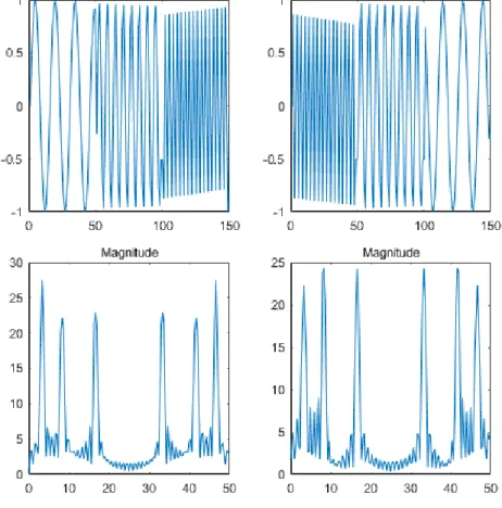
In the following experiment the VSC-HVDC experiences DC line to ground faults (DCLG) at various location. In the 1st case a DC LG fault occurred at 5km from VSC1 side. The fault stars at 2.0s. The DC current data is taken as the input data of wavelet transform, Fig 6.3 shows the 5th level wavelet coefficient.

54

Fig 6.3 coef. of 5th db4 wavelet transform of DC line current (DCLG -5km) In 2nd case a DC LG fault occurred at 2.0s. DC line current coefficients is shown in Fig 6.4. In this case the fault occurred at 15km away from VSC1 side. The maximum value is 62.99.

Fig 6.4 coef. of 5th db4 wavelet transform of DC line current (DCLG -15km) In 3rd case a DC LG fault occurred at 2.0s. DC line current coefficients is shown in Fig 6.5. In this case the fault occurred at 25km away from VSC1 side. The maximum value is 55.06.

55

Fig 6.5 coef. of 5th db4 wavelet transform of DC line current (DCLG -25km) In the 4th case a DC LG fault initialed at 2.0s. The fault is set at 35km away from VSC1. The coef. is plotted in Fig 6.6, where maximum value is 49.61.

Fig 6.6 coef. of 5th db4 wavelet transform of DC line current (DCLG-35km) In the 5th case a DC LG fault 45km away from VSC1 side stared at 2.0s. The coef. current is shown in Fig 6.7. Max coef. is 47.95.

Fig 6.7 coef. of 5th db4 wavelet transform of DC line current (DCLG-45km) In the 6th case a DC LG fault 55km away from VSC1 occurred at 2.0s. The coef.

56

of DC line current is observed in Fig 6.8. The max coef. of DC line current is 44.39.

Fig 6.8 coef. of 5th db4 wavelet transform of DC line current (DCLG-55km)

Fig 6.9 coef. of 5th db4 wavelet transform of DC line current (line to ground) Table 6.3 shows the absolute value of coef. of the DC line current under faults with different locations on the transmission line. These ranges of coefficients value can be used for the detection of the fault. The change of the DC L-G fault location has an obviously influence on coefficients. coefficients are different at different fault location. coefficients decrease as the distance increases.

Table 6.3 Absolute value of coef. of the DC line current under faults with different locations on the transmission line

Location 5 15 25 35 45 55

57

But for more accurate detection wavelet entropy principle analyses can be carried out for further analysis. Table 6.4 show the wavelet entropy of 5th db4 wavelet of the DC line current under faults with different location.

Table 6.4 The wavelet entropy of 5th _{db4 wavelet of the DC line current under faults} with different location.

It can be observed that when a DC fault happens at 5 km from VSC1, the entropy is - 2.68E+07. With the changing of the fault location, there are obvious changes on the wavelet entropy. From the table it is clear that if the fault distance is increasing from rectifier side the entropy is increased.

6.4 Fault detection using wavelet transform in VSC-HVDC DC LL fault

In the following experiment the VSC-HVDC experiences DCLL faults at various location. In this research the fault locations are set at 15km, 35km and 65km away from VSC1 side.

In 1st _{case a DCLL fault occurred at 15km from the VSC1. The fault is set starting} at 2.0s The DC current data is taken as the input data of wavelet transform., the coef.

Location 5 15 25

Wavelet entropy -2.683E+07 -1.696E+07 -1.278E+07

Location 35 45 55

58 of DC current is plotted in Fig 6.10.

Fig 6.10 coef. of 5th db4 wavelet transform of DC line current (DCLL-15km) In the 2nd case, change the location of DCLL fault from 15km to 35km away from VSC1. The starting time is set the same as case 1. coef. of IDC is indicated, where maximum value is5.99.

Fig 6.11 coef. of 5th db4 wavelet transform of DC line current (DCLL -35km) In the 3rd _{case, a DCLL fault started 2.0s after the simulation begins, which is set} 65km away from the VSC1. The coef. of DC current is shown in Fig. 6.12. the max coef. is 5.91.

59

Fig 6.12 coef. of 5th db4 wavelet transform of DC line current (DCLL -65km)

Fig 6.13 coef. of 5th db4 wavelet transform of DC line current (line to line) Table 6.5 and Table 6.6 show the coef. of the DC line current and the wavelet entropy of 5th _{wavelet of the DC line current and wavelet entropy of 5}th _{db4 wavelet of} the DC line current under faults with different location. The result analysis can prove the conclusion from the fault detection using wavelet transform in VSC-HVDC DC line to ground fault.

With increasing of distance from VSC1, max value of coefficients and wavelet entropy change significantly. With increasing faults distance from 15km to 65 km, max value of coefficients is 6.08 at 15km, 5.91 at 35km and 5.51 at 65km which decreases with the increasing distance. Wavelet entropy are -9.8235e+04 at15km, -5.7382e+04 at

60

35km and -3.5559e+04 at 65km which increasing with the increasing distance.

Table 6.5 The absolute value of coef. of the DC line current under line to line faults with different locations on the transmission line

Table 6.6 The wavelet entropy of 5th _{db4 wavelet of the DC line current under line to} line faults with different location.

Location 65 35 15

Max value of coefficients 5.51 5.91 6.08

Location 15 35 65

61

Chapter 7 Comparison between wavelet method and

particle filter method

Data analysis and processing of nonlinear, non-Gaussian stochastic systems have practical applications in the fields like statistics, image processing, computer vision, machine learning and automatic control.

7.1 Introduction

In the past, due to the requirements of signal processing and computational storage, recursive filtering algorithms are usually used to solve such problems, namely the so-called Kalman filtering theory. The basic idea is to approximate the nonlinearity of the system by parameterized analytical expression to obtain needed estimation accuracy. However, the extended Kalman filter is only suitable for the case where the filtering deviation and the prediction deviation are not big. The extended Kalman filtering of the modified gain is improved by the gain matrix. Correspondingly, the estimation performance of the state covariance is improved, but it has certain limitations on the measurement error. If the measurement error is large, convergence accuracy of the algorithm is not good. And convergence time and stability are not ideal. And both of the two filters only use the first-order partial derivative part of the nonlinear function Taylor expansion (ignoring the high-order term), which often leads to large deviations in the estimation, affecting the performance of the filtering algorithm. In short, theoretically, a linear system with measurement noise are Gaussian, Kalman filtering can obtain the optimal state estimation; when the above conditions are not met, the

62

filtering and prediction accuracy will be difficult to guarantee. Therefore, for a nonlinear, non-Gaussian state model, if it is still simply like the Kalman filter theory, only using the mean and variance to represent the state probability distribution will result in poor filtering performance.

Particle filtering is a statistical filtering method. According to empirical situation of system, group of random samples is generated to become the initial simples in space. These samples are called particles; then the weight and position are revised after observation, and the original empirical condition distribution is corrected by the information of the adjusted particles. Particle filter is considered as a good method when facing nonlinear problem

Particle filters have been applied in current researches in system fault diagnosis. In [64], an nonlinear and no gaussian system is studied, and particle filter is applied in this research on fault detection. In [65] the author studied fault detection of an nonlinear system, in this research a particle filter based method is introduced.

7.2 Fault analysis using PF

In this research, basic particle filter-based method is considered in VSC-HVDC fault analysis, the results are used to compared with the results from wavelet analysis-based method in HVDC faults analysis.

Table 7.1 PF based HVDC fault anlysis

Normal ACLG ACLLG ACLLLG

Max xpart(i) -13.57 9.774 -13.73 -13.74

Min xpart(i) -16.13 -12.2002 -15.17 -15.12

Particle filter

63 7.3 Conclusion

Analysis the results, this particle filter based VSC-HVDC fault analysis method is not as good as wavelet based HVDC faults analysis method. When HVDC system experience an HVDC fault, we can judge the occurrence of HVDC system faults from the results of max xpart(i), min xpart(i) and the root mean square (RMS) error. When no HVDC fault occurs, the max and min xpart(i) and RMS error are -13.57, -16.13 and 1.6033. When AC single line to ground fault occurs, RMS error has a significant increase to 7.1725. When other HVDC faults (ACLLG, ACLLLG, ACLL, ACLLL, DCLL, DCLG) occurs, RMS error of these faults have a significant decrease, where the result of AC two lines to ground fault is reduced to around 1, the result of DCLL fault is reduced to around 2, results of other faults are reduced around 0.5. From this result, RMS error can be used in judging the occurrence of HVDC system faults especially AC single line grounding fault, AC double line grounding fault and DCLL fault. However, when a fault other than the above three faults occurs, particle filter based HVDC fault analysis method can diagnose the occurrence of a fault but cannot determine the specific fault type. In this respect, wavelet based HVDC fault analysis

ACLL ACLLL DCLG DCLL

Max xpart(i) -13.74 -14.04 -14.09 -11.39

Min xpart(i) -15.12 -15.70 -15.61 -15.14

Particle filter

64

65

Chapter 8 Conclusion and future work

To diagnose HVDC faults fast and accurately, when HVDC system experiences various faults, this research has proved that wavelet transform based HVDC faults analysis method is a feasible and efficient fault analysis technology.

The wavelet transform can detection the changes in HVDC signals. WT is applied to analyze HVDC faults. Classification of both HVDC DC faults on transmission lines and HVDC AC faults at convertor side and invertor side using wavelet transform is achieved.

Based on the achievement of HVDC faults classification, this research studied on DCLL fault and DCLG fault at various location. Db4 wavelet at 5th _{level has been} applied in DC faults detection. The results proved that wavelet transform can detect the location of DC faults.

For more accurate results, wavelet entropy has been applied in this research. The results indicate that wavelet entropy changes with the changes of location of HVDC DC faults on DC line, which is useful as a reference in detecting HVDC fault locations.

In the future, more detailed research and some other aspects of fault detection and diagnosis in HVDC need to be studied.

1) This research focus on VSC-HVDC system. However, only study VSC-HVDC is not enough to achieve the stable operation of all HVDC system, for LCC-HVDC and MMC-HVDC are still been applied in power system. in future study, wavelet based HVDC fault diagnosis and detection research will be study in LCC-HVDC

66 and MMC-HVDC.

2) In this research AC and DC faults at system level are considered. However, in the operation of HVDC system, there are other faults that need to be study like convertor, invertor, submodular fault in HVDC, etc. in future study, the type of fault being diagnosed will expand.

3) In future study, wavelet transform will be combined with other methods for fault analysis in HVDC.