Finding the best statistical model to predict customer defection in telecommunication retail setting

(1)

Finding The Best Statistical Model

To Predict Customer Defection In

Telecommunication Retail Setting

Nkululeko Ngcongo

February 11, 2014

University of Witwatersrand Supervisor: Prof. David Lubinsky

Student Number: 576639

A Research Report submitted to the Faculty of Science, University of the Witwatersrand, Johannesburg, in partial fulfilment of the requirements for the degree of Master of Science

(2)

Candidate’s Declaration

I, Nkululeko Ngcongo, declare that this Theses is my own, unaided work. It is being submitted for the Degree of Masters of Science at the University of the Witwatersrand, Johannesburg. It has not been submitted before for any degree or examination at any other University.

Nkululeko Ngcongo 11 February 2014

(3)

Abstract

In this study we examine the question of which statistical mod-els work well in predicting customer defection in the retail mobile telecommunication industry. For each of the two data sets that were used (mobile call pattern and billing, and time taken to churn data), four statistical models were fitted and compared namely; artificial neural networks, decision trees, logistic regression and support vector machines. The artificial neural network model proved to be supe-rior than the other three models when fitted on both data sets. This model gave the best area under the receiver operating characteristic curve (0.93 for call pattern data and 0.88 for billing and time taken to churn data), highest lift at 10 per cent of the population (7.01 for call pattern data and 2.12 for billing and time taken to churn data) and lowest misclassification rate (0.04 for call pattern data and 0.19 for billing and time taken to churn data). The logistic regression model under performed the other models when fitted to call pattern data and came out as third when fitted to billing and time taken to churn data whereby they outperformed the decision tree model. Support vector machine came out as the second best model for billing and time taken to churn data and third when fitted to call pattern data. Decision tree model performed well when fitted to call pattern data and worst when fitted to billing and time taken to churn data The study showed that in the retail mobile telecommunication industry, companies can increase revenue streams and competitive advantage by using data mining techniques to predict customers that are likely to churn. The next step for the business is to embark on retention programs to use these methods to reduce churners.

(4)

Dedication

This thesis is dedicated to my family, friends and all the under privileged children trying to strive in the ghetto.

(5)

Acknowledgments

I would like to thank my supervisor Professor David Lubinsky for dedicating his time and guiding me with my work. I would like to send my sincere thanks to my family for being supportive and understanding all the time. Another great thanks goes to all my friends especially Njabulo Ngcongo, Sivuyile Mgobhozi, John Mukombewrana and Nompumelelo Zama for their support and assistance. A great thanks also goes to the University of Cali-fornia and Data Mining Inc. for their data sets.

(6)

List of Figures

1 Plane separating the data points . . . 7

2 A typical artificial neural network . . . 10

3 Logistic and hyperbolic tangent sigmoid functions . . . 11

4 A feed forward neural network with two hidden layers . . . 12

5 ROC Curve . . . 14

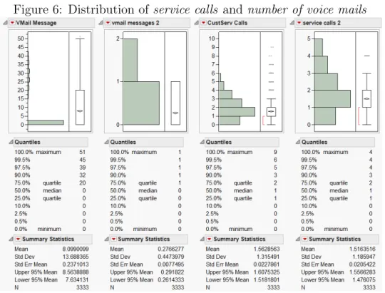
6 Distribution ofservice calls and number of voice mails . . . . 40

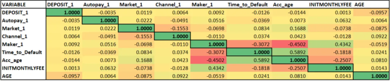
7 Correlation table for data set two . . . 42

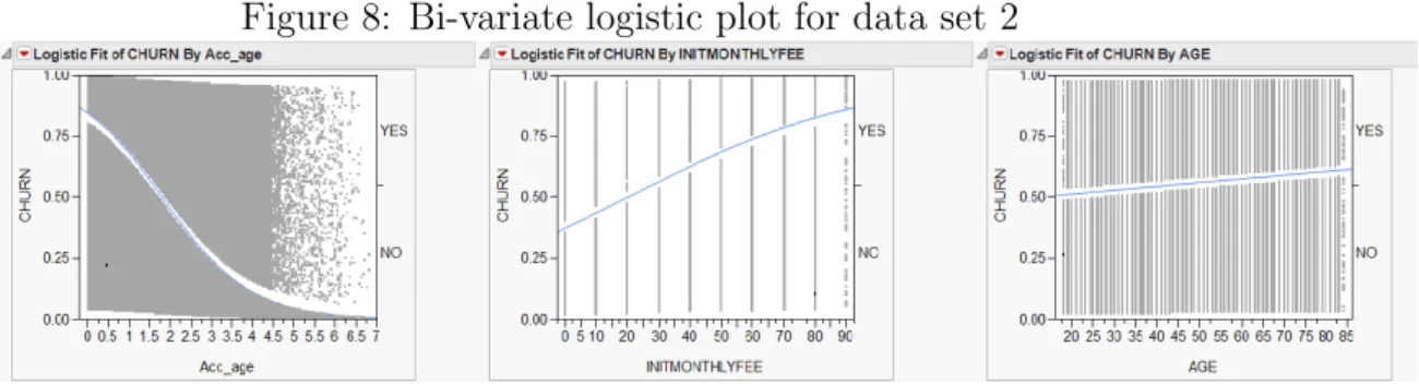
8 Bi-variate logistic plot for data set 2 . . . 44

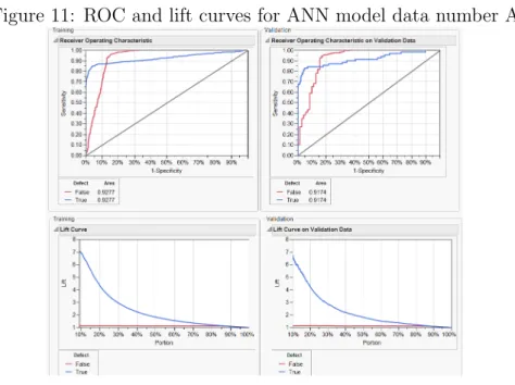
9 Lift curves for the six neural networks before data transformation 48 10 Lift curves for the six neural networks after data transformation 48 11 ROC and lift curves for ANN model data number A . . . 50

12 ROC and lift curves for ANN model data number F . . . 51

13 Number of Decision Tree Splits . . . 53

14 Decision trees variable importance data set 1 . . . 54

15 Support vector constant effect 1: RBF kernel function . . . 55

16 Support vector constant effect 2: RBF kernel function . . . 56

17 Support vector machines ROC curve fit for data set 1 . . . 57

18 Probability cut off for data set 1 SVM model . . . 58

19 Probability cut off for logistic regression data set 1 . . . 60

20 ROC and lift curve for logistic regression data set 1 . . . 61

21 AUC for ANN models . . . 63

22 R-Square for a change in the number of hidden units in ANN model . . . 64

23 Sensitivity for a change in the number of hidden units in ANN model . . . 64

24 Misclassification rates for a change in the number of hidden units in ANN model . . . 64

25 Decision trees R-Square value per split for data set 2 . . . 66

26 Decision trees lift curves for data set 2 . . . 67

27 ROC fit for kernel SVM models data set 2 . . . 68

28 Probability cut off for data set 2 SVM model . . . 69

29 Probability cut off for logistic regression on data set 2 . . . 71

30 ROC and lift curve for logistic regression on data set 2 . . . . 71

A1 Data set 1 distribution A . . . 83

A2 Data set 1 distribution B . . . 83

A3 Data set 1 distribution C . . . 84

A4 Data set 1 bi-variate logistic fit . . . 84

(9)

A7 Data set 1 kernel SVM fit . . . 86 A8 Data set 2 kernels SVM fit . . . 86 A9 Correlation table for data set 1 . . . 87

(10)

List of Tables

1 Model Comparison . . . 3

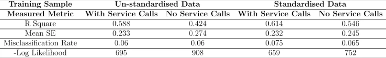
2 Training sample results for standardised and un-standardised data . . . 46

3 Test sample results for standardised and unstandardised data . 46 4 Neural networks results before transforming the data . . . 47

5 Neural networks results after transforming the data . . . 47

6 Sample Test and Train Ratios . . . 49

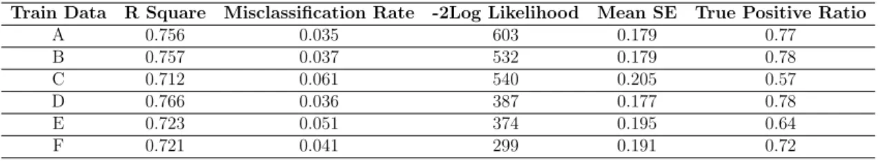
7 Train data model performance for data set 1 . . . 49

8 Test data model performance for data set 1 . . . 49

9 Train data model performance for data set 2 . . . 61

10 Test data model performance for data set 2 . . . 62

11 Data set 1 model comparisons . . . 73

12 Data set 2 model comparisons . . . 73

A1 Data set 1 variables . . . 81

(11)

Abbreviations

ANN = Artificial Neural Networks SVM = Support Vector Machines Data set 1 = Call pattern churn data

Data set 2 = Billing and time taken to default data RBF = Radial basis function

SMOTE = Synthetic minority over sampling technique ROC = Receiver operating characteristic

AUC = Area under the curve AIC = Akaike information criteria BIC = Bayes information criteria SBC = Schwarz Bayesian criteria

(12)

1 Introduction

1.1 Background

Statistical data mining is the process of extracting data from different data sources and manipulating the data in order to produce meaningful informa-tion that can be used by management to make decisions. Data mining is an ’emerging’ field in statistics since technology has allowed us to store large amounts of data to be analysed so that companies, governments and other or-ganizations can make informed decisions. Statistical data mining techniques can be applied to many social science fields [Chow, 2002, Kvam and Sokol, 2004, Crang, 2002, Philip et al., 2011, Mazzocchi, 2007, Juahiainen, 2012]. In this research, we concentrate on using statistical data mining techniques in the marketing field. Marketing departments around the world have huge databases with customer’s demographic and behavioural details. They no longer need to rely on gut feel, rather they can use statistics in order to make informed decisions. In the case where the industry has reached satu-ration the market becomes a churn market and it is difficult and expensive to recruit new customers [Friedman, 1997]. In order for a business to survive fierce competition where churn rates are high, it must rely on statistical data mining techniques to predict churners. Statistical data mining has played an important role in market research in recent years [Imhoff, 2001].

In the retail mobile telecommunication setting, customer relationship man-agement is a very important aspect of the business. Customers have a fixed contract with a known expiry date or termination date. Not all customers will be satisfied with the service they receive and this will lead to customers not renewing their contracts or terminating them earlier than expected. There are various factors that will lead to this, for example:

• Bad service

• Better offers by competitors

• Network inefficiencies

There are also some exogenous factors that one cannot account for that can lead to customer defection, for example:

• Deceased or emigrated customers

(13)

• Fraudulent contracts that need to be terminated

• Natural disasters

Because retention efforts are expensive, it makes sense to look at retention initiatives for only high value customers. A high value customer may be determined based on the following factors:

• Their ’age on book’ is at least more than the initial contract period (excluding new customers)

• They have never missed any of their monthly instalments

• They have participated in a customer satisfaction survey or other study

• They have at least one of the top of the range products

• They must have at least renewed their contract once

• They have not opted out of marketing initiatives

1.2 Statistical problem: finding the best model

The main research question that we address is which statistical technique predicts with accuracy the ’high value’ customers that are likely to defect in the retail mobile telecommunication setting. In this problem of predicting customer defection, we are not highly concerned about time taken to defect but mainly concerned about detecting a type of customer profile that is likely to defect. The aim is to predict defection or termination of the service by customers and to also understand the type of statistical techniques that are most successful in predicting customer defection in this setting. This will enable us to classify with a certain probability whether customers are likely to defect or not, based on their historical data.

The retail mobile telecommunication setting is highly competitive therefore, it is easy for a customer not to renew his or her contract. If no new high value customers are recruited as the old ones that churned, then there will be a significant decrease in profit margins. This will lead to business insol-vency.

(14)

2 Statistical Theory

2.1 Models to be used

The following standard data mining classification models were used in this research to predict churn:

• Artificial neural networks

• Decision trees

• Linear support vector machines

• Logistic regression

The motivation behind using these models is their simplicity and it is fairly easy to interpret the results. We want to find out which model is the most suitable for dealing with retail mobile telecommunication data. Table 1 shows the basics of the four models. Yang and Chiu argued that artificial neural network models are a black box and that the weights of the neurons are un-interpretable. This is a big disadvantage compared to the other three models [WSE, 2006].

Table 1: Model Comparison

Model Decision trees Logistic regression Support vector machines Artificial neural networks Loss Function Confusion Matrix Log Loss Hinge Loss Log

High Dimen-sional Feature

Linear Kernel Gaussian Kernel Polynomial Hyperbolic Tangent Works Well

With

Continuous and Binary Binary Continuous Continuous and Binary Over fitting Pruning Cross Validation L2_Norm _{Early Stopping}

In the remainder of this section we will introduced each modelling tech-nique.

2.1.1 Decision Trees

The basic idea of decision tree models is that for a given training sample d ⊂ D, where D is the entire data set containing Xi, ∀i = 1,2,· · · , n

in-dividuals with k attributes and n >> k, you want to divide d based on the kth _{attribute and the class} _j, _∀_j _{= 1}_,_{· · ·} _{, f} _{you wish to predict such that}

(15)

class j is the response variable which can be binary or has multiple states. Suppose that the class variable that you wish to predict is the likelihood that a customer will terminate his/her cell phone contract with a certain service provider (good = not terminate, bad = terminate). The training sample d will be used to build the tree and the model derived from d will be used to classify the Xi in the test sample T =D−d. Using the test sample you can

also check the model accuracy by checking how many individuals you have correctly classified. The model will enable you to classify new data points entering the system as to whether they will terminate or not.

The decision tree technique is widely used in the data mining industry and is well known for its simplicity. To decide which variable to split on, many functions have been suggested. The most common are GINI index, entropy and information. When a node p is split into l partitions, the quality of the split is given by GIN Isplit = l X j=1 P(kj)GIN I(p/k) (2.1)

where k is the attribute used to split into class j and GINI index at node p is GIN I(p) = 1− f X j=1 (P rob(j/k))2

where P rob(j/k) is the probability of class j at node p. A pure node is reached if GIN I(p/k) = 0 and a best split is the variable with the lowest GINI index [Linoff and Berry, 2004].

The entropy of a random variable Xi, i= 1,2,· · ·, n is

entropy(a1, a2,· · · , aj) =−a1loga1−a2loga2 − · · ·,−ajlogaj

which is

=−Xajlog(aj),∀j = 1,· · · , n

where aj is the probability thatXi belongs to a class j.

Let d be the training data set, j be the class that you want to predict (cus-tomer terminates contract or not) and k the data attributes and entropy function g(x) then the information gain is:

Inf o(d, k) =g(x)−X i

|Yi/kattribute|

(16)

The information gain has a huge disadvantage when it comes to splitting data with distinct or unique values as these carry the highest information in the data set (This means that the data will be split first by this variable thus showing it as the most significant variable). The k attribute with the highest information gain will be used to split the data [Kamber and Han, 2006]. Proust suggested that one can also split on the G squared statistics which works out to be twice the size of entropy, that is G2 = 2∗entropy [Proust, 2012].

2.1.2 Logistic Regression

The second classification technique that was considered was logistic regres-sion. The basic idea is that you have a data set ofn distinct individuals with Xi,∀i = 1,2,· · · , n and you want to predict each individual belonging to a

certain class j (terminate phone contract = bad or not terminate = good, say) with a certain probability. Let j =class where j = 1 if good and 0 if bad and let X=X1,· · · , Xn be the observed data set variables then

P(j =Class|X=Xi) =

exp(β0+β1X1+· · ·+βnXn)

1 + exp(β0+β1X1+· · ·+βnXn)

(2.2) is the probability of belonging to a certain class [Friedman et al., 2008]. It must be noted that the exponent part is the normal multivariate linear equa-tion where you can have dummy variables, indicators or interacequa-tion terms. Not all attributes for Xi points will be significant in predicting the

member-ship of a class j, you can therefore select the attributes that are significant in predicting class j. This may be done by a forward or backward selection method. After fitting the logistic model the contribution or significance of each selected attribute to the model can be determined by likelihood ratio test or the Wald statistic and other methods [Cios et al., 2007].

The odds ratio is used to measure the association between response and predictor variables, that is, the probability of occurring versus not occurring. The odds ratio is widely used in Bio-statistics for evaluating association and relative risk of a certain factor for the groups being studied [Raygoza, 2009]. Suppose two groups are being studied (control and treatment group) and let ¯T be the probability of an event in the treatment group and C be the probability of an event in the control group then the odd ratio is:

¯ T

(17)

IfOR= 1 then the odds of the event being studied are equally likely to occur in both groups that is the probability of each event occurring is half. This lead to the following equation

P(j =Class|X=Xi) = OR 1 +OR which means that

OR= P(j =Class|Y =Yi) 1−P(j =Class|X =Xi)

The odds ratio can be studied for each variable in the logistic regression and this measures the contribution of that variable to the regression equa-tion.

2.1.3 Support Vector Machines

The third technique considered was the support vector machines (SVM). The basic idea is that you have a training sample d and data points Xi, i=

1,2,· · · , n and you want to divide the data set into j regions (j may be the class variable). The data will be divided by a set of hyper planes into j regions [Mirowski et al., 2008]. The support vectors are the data points that are closest to the plane that divides the data into j sub regions. You may have quite a large number of the hyper planes that divide the data intoj sub region but what you really want is a hyper plane (line) that maximizes the region between the support vectors [Friedman et al., 2008]. This is because maximising the region between the support vectors decreases the likelihood of misclassifying new data points.

(18)

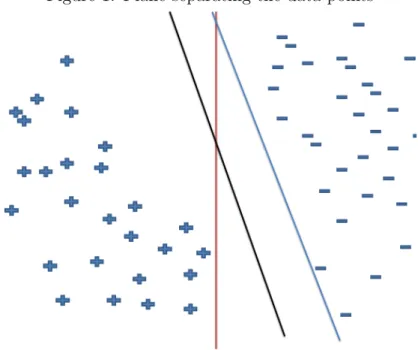
Figure 1: Plane separating the data points

Figure 1 shows three planes that can separate the positive and negative data points with zero misclassification rate [Mirowski et al., 2008]. From this fig-ure, the black plane is the best separator because it gives a bigger margin between the two groups of points. A bigger margin is best because there is a higher chance that if a new data point is imputed it will be classified correctly. Finding the best plane (line) that separates these points is an optimisation problem which can be solved using Lagrangian methods. Sometimes these data points may not be linearly separable.

To define this in a mathematical way, suppose you have a training data set

D= [(x1, y1),(x2, y2),· · · ,(xl, yl)],∀xRn, y[−1,1]

wherexl_,_∀_i_{= 1}_,₂_,_{· · ·}_{, l} _{is the vector of individual and attributes, and}_yl _are

regions of belonging for each individual Xn_{. These points can be separated}

into −1 or 1 by a hyper plane< w, x >+b= 0 where b is the distance from the point to the plane,wthe weights vector and< w, x >is the dot product. The separating hyper plane must satisfy

(19)

d(w, b;x) = |< w, x

i _>₊_b_|

||w|| (2.4.2)

The optimal hyper plane is the one that minimises φ(w) = 1₂||w||2 _and com-bining this with 2.4.1 and forming a Lagrangian equation with parameter alpha it leads to finding a solution of

φ(w, b, α) = 1 2||w|| 2₋ l X i=1 αi(yi[< w, xi >+b]−1) (2.4.3)

which satisfies the Karush Kuhn Tucker condition which is first order condi-tion for an optimal value. From 2.4.3 one must find the first partial derivative with respect to b and w and equate to zero for an optimal solution. The so-lution to the problem is then given by

α‘=argminα 1 2 l X i=1 j X i=1 αiαjyiyj < xi, xj >− l X k=1 αk (2.4.4) constrained by αi >0 and Pj i=1αjyi = 0

Assume now that the data is not linearly separable by a hyper plane and suppose now that there is an error ψi,∀i = 1,2,· · · , l then the constraint

equation 2.4.1 will be modified to

yi[< w, xi >+b]>= 1−ψi,∀i= 1,2,· · · , l (2.4.5)

and the optimal plane is found by w that minimises φ(w, α) = 1 2||w|| 2₋_C l X i=1 ψi (2.4.6)

where C is given subject to constrains. The Lagrangian equation now be-comes φ(w, b, α, ψ) = 1 2||w|| 2₊_C l X i=1 ψi− l X i=1 αi(yi[wTxi+b]−1 +ψi)− l X j=1 βiψi (2.4.7) where β and α are Lagrangian multipliers. The equation 2.4.7 is solved in similar fashion to 2.4.3 and the solution is given by

α‘=argminα 1 2 l X i=1 j X i=1 αiαjyiyj < xi, xj >− l X k=1 αk (2.4.8)

(20)

constrained by 0<=αi <=C and

Pj

i=1αjyi = 0 [Gunn, 1998]

Now that the optimisation problem is solved one needs to know the type of hyper plane to be fitted. When fitting a SVM model one can use kernel functions to map the data into high dimension with the aim of making the data more separable. There are quite a number of kernel functions that are available but we will look at the following kernels:

• Radial Basis Function: k(x, x‘_{) = exp(}₋_σ_||_x₋_x‘_||2₎ • Polynomial: k(x, x‘) = (scale < x, x‘>+K)N

• Hyperbolic Tangent: k(x, x‘_{) = tanh(}_{< x, x}‘_>₊_K₎ • Laplace: k(x, x‘) = exp(−σ||x−x‘||)

and the choice of the kernel really depends on the data set. The parameter choices of K, N (degree) and σ also depends on the data set. Furthermore, in R (A statistical analysis software) if these parameters are not given, the program will select the best ”parameter” values for you [Karatzoglou et al., 2006].

2.1.4 Artificial Neural Networks

The final model that was used in this research was artificial neural networks (ANN). The reason behind using this approach was that it can fit the data well where linear and other models have proved inadequate. The drawbacks are that this model tends to over fit the data and the fact that it is complex to execute and interpret at times. This data mining classification technique was inspired by biological nervous system architect [Nemati, 2000]. In biology, millions of neurons are interconnected by synapses which carry ”information” from one neuron to another. This information is then sent to other neurons as output and the end results are just sensory information (for example: jump). Data mining construction of a neural network uses almost similar ideology to biology in the sense that you have the following:

• An output vector that passes information

• A ”neuron” that processes this information

(21)

Figure 2: A typical artificial neural network

Figure 2 shows a typical ANN where the xi for i = 1,2,· · · , j are the input

vectors, the wi fori= 1,2,· · · , j are input vector weights and

Σ =

j

X

i=1 wixi

is the sum of each weight times the input vector [Cheng and Titterington, 2000]. Let yi =Pj_i₌₁wixi be the net input of a neuron then there exists an

activation function that gives an output, that is

f(yi) = h( j

X

i=1

wixi) (2.5)

wheref(yi) is the output fromha sigmoid or linear activation function. The

sigmoidal function can be of the form of a hyperbolic tangent, logistic, radial basis function etc. A sigmoidal function is an S shaped curve.

(22)

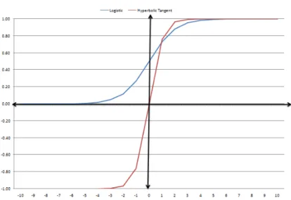
Figure 3: Logistic and hyperbolic tangent sigmoid functions

Figure 3 shows logistic (in blue f(xi)log) and hyperbolic tangent (in red f(xi)tanh) sigmoidal functions [Turhan, 1995]. The logistic sigmoid is

asymp-totic to the lines f(xi) = 0 and f(xi) = 1 while the hyperbolic tangent

sigmoid is asymptotic to the lines f(xi) = 1 and f(xi) = −1. The two

sigmoid functions are continuous and differentiable on xi[−∞,∞] interval

[Turhan, 1995]. Furthermore, f(xi)tanh = 2f(xi)log−1 (1) = 2 1 + exp(−xi) −1 (2) = 1−exp(−xi) 1 + exp(−xi) (3)

In this research, we looked at a feed forward artificial neural network and used the hyperbolic tangent as a sigmoidal function. A feed forward neural network has a hidden neural network structure such that the message gets passed from the first neuron to next one but the message is not returned back.

(23)

Figure 4: A feed forward neural network with two hidden layers

Figure 4 shows a typical feed forward neural network architecture where the w’s are the weights of each neuron,Y is the output and thex’s are the input vector. When fitting an artificial network model we try to find the unknown weightswj by minimising the error of the output from the estimated weights.

Optimisation techniques such as Back-Propagation, Newton-Raphson and other techniques are used to estimate the wj. Two problems that may arise

from fitting ANN is getting the starting values of the weights to be estimated and over fitting the neural network model. A zero value can be used as a starting point of estimating weights and the early stopping rule in the optimisation technique can be used to avoid over fitting.

2.2 Model evaluation

We evaluate the models using; Bayes Information Criterion (BIC), Receiver Operating Characteristic Curve (ROC), Akaike Information Criteria (AIC), misclassification rates and the lift charts because these are the commonly used evaluation criteria methods.

2.2.1 Bayes and Akaike Information Criterion

The AIC and BIC measure the performance of a statistical model for a data set being analysed. These models depend mostly on the likelihood function and will penalise models with higher numbers of parameters. The main idea is to see which models are over fitting the data amongst the ones that are being compared. These measures are calculated as below:

(24)

AIC =−2 log(l) + 2k (2.6) and

BIC =−2 log(l) +klog(n) (2.7)

where l is the likelihood value, k is the number of parameters and n is the total number of observations. As the model becomes more complicated, k number of parameters used to estimate the model will increase, the AIC and BIC values will increase and the model will be over fitting the data.

2.2.2 Receiver Operating Characteristic Curve

The ROC curve measures how well the model fits by plotting the false positive and negative fraction and evaluating the area under the fitted curve. Given that we have a class that we want to predict (that is, customer defecting or not) and a given set of data divided into training and test sample. The model is built on the training sample and evaluated on the test sample. For the ROC curve we will be looking at the

following:-• True Positive and Negative Fraction: Predicted to defect in the training sample and actually defected and predicted not to defect and actually not defecting

• False Positive and Negative Fraction: Predicted to defect but does not defect and predicted not to defect but defect.

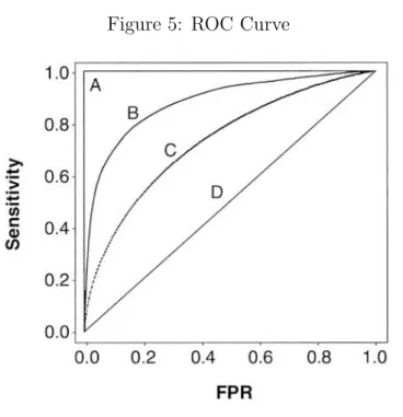
A best fitting model is the one with the lowest error rate, that is, with low false positive fraction. As a retail mobile telecommunication company you would want to reduce these errors. The ROC curve is then a plot of sensitivity(true positive rate) versus 1−specif icity(true negative rates/false positive rates). Figure 5 shows a typical ROC curve.

(25)

Figure 5: ROC Curve

The 45 degree line (y = x which is labelled D) signifies a worthless model, curve C show that the model is performing better, curve B is better fitting test and curve A is the perfect model [Zou et al., 2007]. The higher the area under the ROC curve the better is the performance of the model. The AUC (area under the ROC curve) is an element of the set [0,1] [Gatsonis, 2008]

2.2.3 Lift Charts

The idea of the lift chart is that as a marketing firm you do not want to email or SMS all your customers for a promotional offer. Imagine doing this for a base of 1 million customers at a cost of 20 cents and only 500 customers respond to the offer of R10. The cost of sending these SMS’s will not be recovered in this case, thus the business will lose a lot of money. The lift chart assists the business in identifying and selecting only the top customers that are likely to respond to the marketing offer rather than using random selection. Measuring a statistical model using the lift curve is done by rank-ing customers with the highest probability of respondrank-ing and evaluatrank-ing the number of the correct predicted customers that actually respond to the cam-paign at a certain population proportion.

(26)

To define this in detail, let Sc be the percentage of customers with highest

ranked probability of churning when selected and P0 be the proportion of customer selected from the whole population of churners and non-churners then

Lif t(P0, Sc) =P0/Sc

As the proportion of the population selected increases, the lift value tends to 1 and in fact

Lif t(100, Sc) = 1

and the maximum lift attainable is 1/Sc [Kno, 1999]. A lift of a random

(27)

3 Literature Review

The research involved looking at relevant literature and detailed review of sixteen papers by the researcher that focused on churning of customers in industries such as banking, telecommunication and other retail sectors. One of the paper reviewed concentrated on sampling techniques when a class of interest is rare. We have applauded and questioned some of the literature based on their approach toward solving the churn problem.

3.1 Credit Card Churn Forecasting

In this research two data mining techniques were used to build a churn pre-diction model using credit card data from a Chinese Bank [Nie et al., 2011]. The authors defined data mining as discovering knowledge and patterns from a large data set. They argued that it costs a lot to acquire new customers so it is important to retain existing high value or profitable customers. In the paper they argued that a bank can increase profits by up to 85 per cent by an improvement of 5 per cent in the retention rate. As the economy develops in China, a large number of credit cards have been issued however most of these credit cards were inactive. With an increased competition in the bank-ing sector, it is easier for a customer to exercise their right of switchbank-ing the product if the current service is not satisfactory.

In this study churn was considered from a customer’s initiation point of view, for example

• More favourable competitor pricing

• False information given to customers from acquisition

• Customer expectation not met etc.

and not by customers that churn because of the bank’s initiation (for example bad debt). A sample of customers was taken from the database and divided into two time frames. A churner was then defined as a customer with no transaction at a chosen time period t (after) and the customer did make a transaction at a previous time t−1 (before). In this paper they used logistic regression and decision trees to predict churn. They also emphasized that these two methods work well in classification problems. The models were validated using percentage of correctly classified, GINI coefficient and ROC curve. They considered two types of

(28)

errors:-• Type 1 error: customer did not churn but is classified as a churner

• Type 2 error: customer churned but were classified as a non-churner The model selection was also based on which model costs the most when selected, that is, the actual currency cost of marketing to the customers that were classified as churners but did not churn. A random sample was selected from a database of 60 million customers from January 2005 to April 2008. The data contained customer’s demographic information, transaction information, abnormal card usage and other transactional activities with the bank. The time period was divided into observation period (where the number of total transactions was counted) and the evaluation period (where they check if the customers that were transacting before are still transacting). Out of 135 variables, only 95 variables were included in the final model. This is because some of the variables were found to be correlated (multi-co-linearity) and this would have affected the model performance if they were included. Logistic regression and decision tree models were compared; they both showed that the demographic variables were not significant in predicting the churn rate. The activity level variables contributed more to significance in the models than the demographic variables and hence the model with these variables performed better than the model without them (for both models). Logistic regression model performed better than the decision trees and gave less cost on error (decision tree cost = 85283 and logistic regression cost = 80377).

3.2 Data Mining Techniques for the Evaluation of

Wire-less Churn

The authors of this article start by explaining the fact that the wireless mo-bile telecommunication industry is very competitive [Ferreira et al., 2004]. As wireless companies grow in numbers customers are faced with wider op-tions to choose from which best satisfy their needs. They explain that there is a battle of advertisement within wireless companies in order to lure cus-tomers to change their mind and switch to utilise their services. Churn was defined as abandoning your service provider as a customer and moving to a competitor. Churn is recognised as a crucial issue in consumer business and economics. The author emphasises that predicting churn beforehand can help in retaining high value customers by giving them counter offers and thus saving the business money.

(29)

Their dataset came from a wireless carrier in Brazil with a sample of one hundred thousand customers and for a time period of nine months. A churner was defined based on termination of service before the ninth month and this was used as a target variable. From the dataset 1.25 per cent was a monthly churn rate which is very small when trying to model customer churn. The authors overcame this problem of very low churn rate by oversampling. This had an implication on the data and the accuracy of the churn model. The authors used the below variables for predicting churn:

• Billing data (roaming cost, revenue, etc.)

• Customer demographic data (gender, marital, region, etc.)

• Customer relationship data (rate plan, handset age etc.)

• Market data (competitor rates etc.)

• Usage data (airtime, data bundles etc.)

In total there were 37 data attributes (behavioural and demographic vari-ables). These variables were transformed and standardised for modelling purposes. The authors then divided the data into two:

• Simple dataset where no modification was done

• Enhanced dataset where the features were reduced using Least Square Estimation and other methods

Using the feature selection methods, it was found that variables related to the airtime consumption by customers were decisive in defining churn. The two data sets were then standardised. The enhanced data representation had 10 variables while the simple data representation had 20 variables. The data was divided into 70 per cent training set, 20 per cent validation set and 10 per cent test set.

Four models were then run on the data set namely neural networks, decision trees, hierarchical neuro-fuzzy system and genetic algorithm rule evolver. The neural network model had optimal number of hidden layers determined empirically and was trained by back-propagation. The cost of each model was evaluated based on the assumption that 50 per cent of the churners that are offered incentive will be retained, the cost of incentive is 25 dollars, average monthly subscription is 80 dollars and only 20 per cent of those predicted as churners are contactable. Based on a total of two million subscribers for this company, results showed that using a neural network model on enhanced data representation can save the company a large sum of money (44.2 dollars

(30)

per client that is likely to churn). The models performed on the enhanced data representation set yielded better results than using a simple data set for all model. Neural network model with fifteen hidden units outperformed the other models.

3.3 Customer Relationship Management at Pay TV

Pay TV is a European company that offers premium channel viewing to subscribers [Burez and den Poel, 2005]. It offers entertainment, news and educational channels to its viewers. Pay TV has a huge database of active customers but in recent years the number of active customers started to decline. It was speculated that the churn was caused by higher fixed cost to customers because it was expensive to maintain Pay TV infrastructure. In this research, they mentioned the following marketing initiatives to try and reduce customer churn

• Give customers free services

• Organising special events to pamper customers

• Survey study on customer satisfaction

In this research, they mention two ways of reducing customer churn. The first of which was an untargeted approach, which is mass marketing to every customer. The second was a targeted marketing approach to customers with a higher probability of churning and provide them with lucrative offers.

Similar to DSTV, if you subscribe to Pay TV you only pay a monthly sub-scription fee. There are no other charges except for pay per view which was not discussed in this research. The subscription is a twelve months contract by which cancellation before the end of twelve months is not allowed. Cus-tomers need to inform Pay TV if they will terminate the contract after twelve months; if this is not done then the contract is automatically renewed. The data was divided into two time buckets that is estimation period (from start of Pay TV to sampling date) and follow up period (a year after the sampling period). Variables that were extracted from the database

were:-• Previous and current subscription

• Demographic (e.g. Age, gender etc.)

(31)

A logistic regression technique was used in this research motivated by its simplicity and because it is widely used in market research. Monthly instal-ments amounts were used as the class variable. Markov chains were also used and the basic was that customers can move from having product 1 (premium say) to a lower product 2 (say compact). Moving within these two states can influence the probability of churning. Random forests were also used as an additional model. The models used were evaluated by Cumulative lift curves and ROC curve. Random forests outperformed other models and gave the best fit and best cumulative lift curve. Furthermore a field experiment was conducted on the customers with a high probability to churn. Customers were given incentives and response was analysed. It was found that the incentive reduced churn significantly.

3.4 Partial Defection of Loyal Clients

In this research the authors discussed customers partial defection from a Fast Moving Consumer Goods non contractual setting [Buckinx and den Poel, 2004]. In this retail setting customers can change their purchasing be-haviour without informing the company about it (for example, in a retail setting where customers do not have loyalty cards). Again, because of high competition in the retail setting it is easy to switch brands. For example, some customers may be price elastic that is, a small increase in price will cause them to switch retailers. They also emphasize looking at customers that are profitable and showing loyal behaviour for retention.

In this research, they looked at two time buckets and looked at behaviour at time 1 and time 2. They then looked at purchasing behaviour in both periods, if there is a change in the negative direction in time 2 then the customer was classified as being partially defected. In this research they used three classification

techniques:-• Logistic regression

• Neural networks

• Random forests

The evaluation criteria used were percentage corrected classified (PCC) and the area under the curve (AUC).

(32)

In this study they selected only the behavioural loyal customers for analysis satisfying the following

conditions:-• The frequency of shopping is above average

• Ratio of the standard deviation σt of the inter-purchase time to the

mean µt inter-purchase time is below average

The data chosen for this study contained customer behavioural and demo-graphic attributes. One may argue that most variables that were used in this study were correlated which may have caused bias in the predictions. Random forest outclassed neural networks and logistic regression techniques. The content of this paper is very powerful in the sense that it looks at par-tial changes in customer behaviour so that corrective initiative can be applied early enough before a customer totally defects.

3.5 Customer Headroom Model

This paper talks about basket analysis in a retail setting in which some bas-kets were believed to have a missing spend [Shashanka and Giering, 2009]. For example, if a customer usually buys only bread in a store yet it is known from previous experience that bread is associated with butter or milk (say) then there is a possibility that the customer is buying these products from another retailer or the customer does not consume these products at all. If a customer has this property then they can make an initiative to try and cross sell products that are highly associated with the ones that are in the customer’s basket.

Customer’s transactional data was extracted for all customers who shopped in the sampled time period using their loyalty cards. Log normal distribution of customers total spend and spend in each item was assumed because the data was skewed. Cross shoppers and customers that buy for large commu-nities were excluded from the analysis as they were outliers and will distort the results. Customers spend, frequency, items bought, number of distinct items bought and demographics variables were used to cluster customers into sub-regions. Each sub-region or segment was modelled on its own for an in-crease in accuracy of the prediction. Singular Value Decomposition was then used to predict customer’s potential spend in each subgroup

(33)

3.6 Churn Prediction Model

The authors explain how costly it is to recruit new customers in mobile telecommunication retail settings where the service providers are faced with high churn rates. Churn is a highly debatable research area not only in mobile telecommunication but also in other industries [Shaaban et al., 2012]. Data mining techniques have helped service providers to reduce customer churn. The authors defined churners as voluntary and involuntary where by volun-tary churn is incidental (unplanned churn) and deliberate (price elasticity, better service and offers). Service providers are concerned with deliberate churn and thus creating a predictive model for this is important. The author mentioned the most frequently used data mining classification techniques with their advantages and disadvantages. These techniques are:

• Decision trees

• Regression analysis

• Neural networks

• Fuzzy logic

The authors sampled 5000 records from a database which was not mentioned and divided it into 80 per cent training and 20 per cent test data set and both train and test data set had a churn rate of 0.2. The data mining and analysis program used by the authors was WEKA. There was a total of 23 variables select from the database and they included demographic, calls and billing data. The authors used decision trees, neural networks and support vector machine for modelling churn and found that neural networks and support vector machine performed better (both 84 per cent model accuracy) than decision tress (78 per cent model accuracy). The authors selected support vector machine as the best model because although the model accuracy rate is the same as neural network model, the support vector machine model is able to pick up more customers that are predicted to churn and they do churn (421 true positives for support vector machines and 403 true positive for neural network model). The authors created three cluster groups of customers (low, medium and high value) based on the 23 variables. We agree with the authors of this paper because:

• It can be clear from the retention program which cluster performs best (more customers are retained)

• Cost can be saved by targeting a cluster that is likely to respond rather that clusters that do not respond

(34)

• High value customers can be targeted since they are loyal and profitable to the organisation

3.7 Churn Prediction in the Mobile

Telecommunica-tion Industry

In this research Alberts started by explaining why was there a need for pre-dicting customer churn [Alberts, 2006]. In the Netherlands there has been a rapid change in the mobile telecommunication industry, from a growing market to saturation and highly competitive market. Therefore most com-panies are no longer investing in acquiring new customers they rather invest in retaining the existing ones. It is easier for a customer to switch from one service provider to another because of high competition. The study was car-ried out for Netherlands Vodafone.

The author used two data mining techniques for predicting churn namely: The Cox survival model and decision trees. These techniques predicted a class of belonging (churner or non-churner) by a certain probability value. In this research the author does not focus on contract customers but only post-paid (prepost-paid) customers. It is also much easier to predict churn for contract customers because the expiry date of the contract is known. In the research churn was defined as stopping to use the company’s services by:

• Voluntary: when the customers switch by choice (say to competitors)

• Involuntary: customers churn because of missed payments or fraud (say)

The proposed research question was the feasibility of modelling churn of prepaid customers using survival and decision tree model. The shortcoming was on how one measures the churn of prepaid customers since there is no specified end date as in a contractual setting. Do survival models have an added value compared to decision tree predictive model? The author defined four states that a prepaid customer can be in:

• Normal use: normal active customers with credit on the prepaid ac-count (1)

• No credit: zero credit in the prepaid account (2)

(35)

• Deactivation: ’churn state’ (4)

A customer can move from state 2 and 3 to the normal state after recharg-ing. In general, it takes longer for a prepaid customer to be disconnected in a network. So in many instances prepaid customers churn before they have been disconnected. The paper looked at prepaid customers that have been completely disconnected.

The data was taken from a Vodafone database and was aggregated monthly for each customer. Twenty thousand customers who joined between April and July 2005 were sampled and analysed. In addition the data contained demographic and activity level with Vodafone variables. Some of the selected variables were:

• Number of months since last recharge

• Number of months since last voice mail

• Ratio of incoming call to outgoing calls

The data was manipulated and it was represented as survival data and then Cox Model was fitted. Some customers churned in the sampled period others were censored. Since survival models are not mostly used for classification or prediction, the author used a specific procedure to do this [Ripley and Ripley, 1998]. A hazard function and instantaneous probability was used for this. A predetermined threshold was used and if the hazard function was above this then these customers were churners [Poel and Larivire, 2003]. On using decision trees the data was divided into test and train sample for validating the model. The splitting criteria or variable importance selection that was used was the GINI co-efficient. The problem of over fitting was avoided by pruning the trees that hold the low information. The decision trees outperformed the Cox survival model but the survival model had an advantage over decision trees in that the survival model takes the time aspect into consideration by means of using a baseline. So the author does not only know which customer will defect but also what is the expected time until the customer defect is.

(36)

3.8 Analysis of Clustering Technique for Customer

Re-lation Management

This paper reviews different types of clustering techniques used in Customer Relationship Management [Manu, 2012]. Manu defines clustering as creating a group of objects based on their features or attributes in a way that the objects belonging to the same groups are similar and those in different groups are dissimilar. He also mentions that clustering plays a significant role in pattern recognition, text mining, web analytics and customer relationship management. Data mining adds a complexity in the sense that you can have a huge data set with many attributes. The way they defined the components of the clustering task was by using the following steps:

• Pattern Proximity: a distance measure on pairs of patterns (there are various distance measures functions)

• Data Abstraction: extracting a data set

• Cluster Validity Analysis: cluster analysis and validating clusters In the paper they represented a feature vector of a single data point as

X = (X1, X2,· · · , Xp)

with p being the dimensions of the space, X is the pattern or vector and the X0s are the attributes. The attributes of this feature vector can be qualitative (nominal) or quantitative (continuous or discrete). In the pa-per they focused on the data with continuous attribute and use Euclidean distance as a measure of similarity (

q Pd

k=1(Xi,k −Xj,k)2). Other texts sug-gest ways of dealing with qualitative data when performing cluster analy-sis [Linoff and Berry, 2004, Friedman et al., 2008]. The author mentioned the disadvantages of having linearly correlated data when clustering which can distort the distance measure. In such instances one can transform the data using whitening transformation or using the Mahalanobis distance dm(xi, xj) = (xi −xj)P

−1

(xi, xj) 0

where xi, xj are row vectors and P

−1 is the inverse of the covariance matrix of thex0s. The author went on to define many clustering techniques with their advantages and disadvantages.

3.9 Churn Prediction in Telecommunications

(37)

munication retail setting [Idrisa et al., 2012]. If high value customers are lost then the company’s revenue will decline significantly. This creates a need to develop a churn probability model that will predict customers that are likely to churn. The authors mentioned that in this setting the dataset has high dimensionality and an imbalanced class distribution. High dimensionality arises from a data set having many behavioural and demographic variables while the imbalance arises from the fact that in general, there are many more non-churners than churners. The imbalance may cause high misclassification rates in the model.

The authors processed the dataset to check for missing values and transform-ing the nominal values. Below is how the data was processed before applytransform-ing the classification methods:

• Dataset with useful fields was extracted from the database

• Useless features are removed and the data was reduced in size using principal component analysis.

• Nominal features (70) were transformed to numerical values by group-ing into three categories

• Data was further processed by applying Random Under Sampling (RUS) and Particle Swarm Optimisation because churn class rate was low (7.3 per cent)

• Principal Component Analysis, Fisher’s Ratio, F-score and minimum redundancy maximum relevance methods were applied for selecting the features to be used in the model.

K nearest neighbour and Random Forest were applied to the datasets in order to predict customers that are likely to churn. These classification techniques were firstly applied to original dataset without any feature selection method applied and then applied to the data set with feature selection methods (four methods). The model performance was evaluated using Area under the Curve (AUC). Random Forest and K Nearest Neighbour performed better when features were selected using minimum redundancy maximum relevance were employed rather than using Principal Component Analysis, Fisher’s Ratio and the F-score. The author concluded by stating that using minimum redundancy maximum relevance feature selection and Random Forest model was efficient for predicting churn in the Telecommunication retail setting where the data set is large and high computational costs are involved. The authors complained about the imbalanced class and did enhance the data by

(38)

using under or over sampling techniques. These techniques did improve the model performance.

3.10 Turning Telecommunication Call Details to Churn

Prediction

A rapid increase in mobile telecommunication service providers has led to high competition [Wei and Chiu, 2002]. In order to survive in such a com-petitive environment businesses nowadays rely on data mining techniques in order to gain advantage over their competitors. The authors of this article mention that churn management and customer retention is the key in busi-ness success in the telecommunication industry. Data mining (information discovery) can be classified into classification, clustering, dependency anal-ysis, data visualisation and text mining as per authors view. In this paper they argued that the use of demographic variables when predicting churn may be misleading because:

• Churn is at customer level rather than contract level as it is common for a customer to have more than one contract

• Often customer databases in mobile telecommunication industry usu-ally don’t have substantial demographic information

They analysed churn data for contract customers by using their call pattern changes. They also argued that using call pattern changes (for example, diminishing incoming or outgoing calls) can be used as a signal for churn. The data was taken from a Taiwanese mobile telecommunication provider which has a monthly churn rate of between 1.5 to 2 per cent. The class variable for this analysis was derived from contract end date. The data contained 114,000 customer call records made between October 2000 and January 2001. This data set excluded customers whose contract was terminated based on delinquency. The authors had prior information about the variable that mostly influence churn from the company managements. These variables were:

• Length of subscriber’s services

• Payment type (debit order or over the counter)

(39)

• Number of minutes for outgoing calls

• Number of outgoing calls made

• Number of distinct people contacted

In the sample data set, a T period was divided into k ”sub-regions” in or-der to evaluate the change in customer patterns. In the data set there are between 1.5 to 2 per cent instances of churn, so the author decided to use multi-classifier class combiner approach. This approach is similar to over-sampling approach in the sense that the small class sample was replicated across different train-test sets while the bigger class was selected at random. A prediction period P was chosen at random from T where churners where defined as having a disconnected status at this period and if the status was active at the end of P then the customers were defined as a non-churner. They also mentioned that there was a retention period R after T and P which allowed the company to offer incentives to keep their customers. They mentioned that data mining techniques are widely used for predicting churn and they used two models (which were not mentioned) on 10 fold cross vali-dation data set. They were mostly concerned about finding the sub-periods where call patterns change and in which prediction period do the models have high accuracy. The model evaluation criteria used were the cumulative lift curves and false alarm rates. The best model gave a lift of 4.68. They also built a model with demographic variables and found that it had a lift of 3.9 which was lower than the lift when no demographic variables are used. It was shown in this research that using behavioural variables for predicting churn is vital and it outperforms the model with demographic variables.

3.11 Churn Prediction Using Complaints Data

In this study the authors explain how valuable it is to maintain existing cus-tomers for the business [Hadden et al., 2006]. They also highlight that it is very costly to acquire new customers and with the rise in competition in the telecommunication industry, customers are likely to move to competi-tors. The authors explained that from past research it has been shown that predicting churn using demographic data is very unstable (Wei and Chiu, 2002). They argued that churn is dependent on customer and not on the contract and so they proposed using call pattern changes. In this paper they took a different approach to this as they predict churn using complaints and repairs data. They used three groups of variables to create the data set namely:

(40)

• Provision data: estimations that are made by the company with regards to resolving a complaint or repair

• Complaint data: information about customer complaints

• Repairs data: fault and repair data

We question the authors because they used only 202 customers to train the model with 50 per cent churners and 50 per cent non-churners whilst the test set contained 700 customers with 70 per cent non churners and 30 per cent churners. This data set was very small for training a model and the class ratios were not the same for both train and test sample. The results might be biased and misleading because the model was built on less churners and tested on data with more churners.

The authors used linear regression, regression trees and neural networks to train the data of 202 customers using Matlab and SPSS. The neural network model was performed by back propagation method with different activation functions and in addition a Bayesian neural network was used. The feed forward back propagated neural network using logistic sigmoid gave the best results when a probability threshold of 70 per cent was used for churners. The authors analysed the weights from the 24 variables that were used to develop the model and found that only seven variables were significant. It was not clear on how this variable significance process was done as the authors did not mention full details. The variables that held the most information were:

• Number of engineers arrived on site

• Customer years on book

• Length of repair

• Number of appointments for repair

• Time to resolve a customer query

• If an order has been placed

• Number of times that a specific repair has been done

The authors then used regression trees in order to assess risk of churning which provided an overall accuracy level of 82 per cent. The regression method performed in SPSS gave an overall accuracy of 81 per cent. Bayesian

(41)

neural network outperformed the other models for predicting churners and the best performing technology was the regression tree technology.

3.12 Churn Models for Prepaid Customers

The author of this article start by highlighting the importance of Customer Relation Management Department in customer retention [Owczarczuk, 2010]. In retention, the company tries to lure back customers that are likely to de-fect and in doing so there are cost associated with the process (marketing material) and bonus if the customer is retained. He argued that the reten-tion projects must not target loyal customers as they will continue using the services of the company. We disagree with the author of this paper because neglecting loyal customers will lead to dissatisfaction and thus loyal cus-tomers will churn. In instances where the loyal customer base is very small and most profit is generated on the ”non-loyal” customers then the author of this paper is correct.

The author worked on predicting churn for prepaid customers rather than contract customer. He argued that it was much simpler to predict churn for contract customers as they have all demographic information about the cus-tomers and the exact expiry date of the contract. The author did not want to define churn in a standard terms used in Poland (SIM expiration). This was mainly because if a prepaid customer makes a recharge in month one of sim card purchase then it takes 365 days of non-use for the card to expire. If the customer recharges a month later then the days to expiry (churn) are re-set to 365 days. The author felt like the period was too long and defined churn as having no incoming or outgoing calls in the last six weeks.

The data set was taken from a Polish mobile provider. It contained two years’ worth of data (2007 to 2008) and it had 1318 variables (behavioural and de-mographics). The author used four models for predicting churn namely:

• Logistic regression

• Linear regression

• Fisher linear discriminant analysis

• Decision trees

(42)

ease of interpretation. They mentioned that random forest and support vec-tor machines as the black-box models which are unsuitable for predicting churn. We criticised the author by saying this because he did not had a valid reason as to why these are black-box models. Again we disagree with the author of this paper because these models may be suitable for a different or much more complex data sets than the one used in the study. The author was very cautious when extracting the data from the database because of attribute data type mix and the fact that on a relational database you do not want to accidentally use primary key field in your model. The author sampled 167,595 records and divided it into 51 per cent train, 22 per cent validation and 27 per cent test set.

The author argued that using regression and Fisher discriminant model in a high dimensional vector may lead to wrong conclusions because multi-co-linearity may arise. Also, there may be computational power problem involved. On each variable the t-test was performed and the variables were ranked according to t-score. The top 50 significant variables were used to fit the models. The model performance was obtained from plotting lift curves of each model in the same axis. Logistic regression performed slightly better than the other models. Decision trees were fitted to full data set (1381 vari-ables) and enhanced data set (50 varivari-ables) and it gave similar results.

3.13 Mobile Telecommunication Handling in India

India has the second largest telecommunication industry in the world with more than 650 million active customers [Jamwal, 2011]. The author ex-plains that in earlier years (1990’s) there were fewer telecommunication ser-vice providers and in recent years there are about 17 serser-vice providers. This has created a lot of competition and the management in the telecommuni-cation industry are mostly concerned and focused on maintaining existing customers. Our opinion differ with the author of this paper and the man-agement because there is natural churn from death, migration and other so recruiting new customers should also be a priority even if the market is sat-urated.

The author was motivated to predict churn because the market has a churn rate of 27 per cent per year. This is very high (more than a quarter of cus-tomers are lost every year), knowing that it is costly to recruit new cuscus-tomers.

(43)

and the reasons behind it. Data mining techniques can help us predict churn from the database thus promoting competitive advantage. The author men-tions that most organisamen-tions lack skills and expertise of data mining and analysis. We agree with the author totally because there is a gap between management and analysts. This gap is because management finds it hard to believe or understand analysts and they may base their decisions on gut feel rather than numbers. The main concern of the author in this research is why do customer churn and who is likely to churn. The author used Chor-diant Predictive Analytics Director software to prepare the data and logistic regression and decision trees for modelling churn. The collected data set se-lected at random had demographic, call details and billing variables of each customer. A total of 15000 customers with a churn rate of 8 per cent were sampled.

From data exploration stage it was found that there was a higher probabil-ity of churn for age group of 45 to 48 than the average churn rate and for the customers whose contract are between 25 to 30 months. The customers that paid low monthly fee are more likely to churn and those that are billed less than 190NT in 6 months. Also customers that have less outgoing calls minutes had a higher probability of churning. From these results the author created KPI’s (key performance indicators) flags on the database to signal customers that are likely to churn. We criticise the author for not mentioning the model that performed the best. Also the sampled data was too small for churn prediction considering the fact the Indian telecommunication compa-nies have huge databases and an average of 27 per cent churn per year and this may create bias in the models used results.

3.14 Knowledge Discovery on Customer Churn

In this paper they reviewed churn in the retail mobile telecommunication space and used the same data set as in this research (data set 1: call pattern data). The author starts by explaining the importance of customer churn in business nowadays [WSE, 2006]. The business need to focus on getting more knowledgeable about its customers in order to maintain a quality ser-vice focus. The study focused on modelling customer churn in a Taiwanese company for prepaid customers who churned voluntary. On the other hand, involuntary churn, that is, customers that churn because of fraud and delin-quency were not included in the analysis. Unavoidable churn customers, that is, customers that churn because of death and migration were included

(44)

in building the model. This is because the mobile service provider cannot differentiate this with voluntary churn.

The authors used a field test to monitor customers after they had been mod-elled as churners. This was different to most churn papers cited in this research. Most of them used historic data to predict churn but do not then monitor the customers that have a higher probability to churn in the next time frame. Below are the steps taken in this research:

• Data extraction in the database

• Data transformation and selection of desired variable

• Sampling for modelling

• Modelling and scoring the whole customer database (on SQL)

For model performance the author used hit rate and lift curves. Decision trees and logistic regression were used as classification techniques because of their simplicity and ease of interpretation. The author criticise using the neural networks for predicting churn heavily saying that the one cannot interpret the weights and calling this model a ”black box”. From the database there were 170 variables selected (containing demographics, billing, usage, call details data etc.) and explored using graphics and chi square. Based on a probability value of 25 per cent (univariate study), variables were reduced to 99. The churn rate in the data set was 0.5 per cent which was very low (but very big when taking into account a database size of more than 1 million records). Due to the low class ratio, the author decided to create bias in train and test data varying the churn rate from 1 to 10 per cent. The best decision tree model was obtained on a churn rate of 2 per cent and a sample size of 375,000. From the list of 5000 customers where a field experiment was conducted a 56 per cent hit rate was obtained. Decision trees outperformed the logistic regression methods. This paper showed that data mining method are applicable even in low churn rates.

3.15 Under-Sampling Approaches for Improving

Pre-dictions

The authors explain that the most important thing in classification problem is to improve accuracy in the training data [Yen and Lee, 2009]. It is normal

Finding the best statistical model to predict customer defection in telecommunication retail setting