Scalable Multilevel Support Vector Machines
Talayeh Razzaghi
1and Ilya Safro
1Clemson University, Clemson, SC (trazzag,isafro)@clemson.edu
Abstract
Solving optimization models (including parameters fitting) for support vector machines on large-scale training data is often an expensive computational task. This paper proposes a multilevel algorithmic framework that scales efficiently to very large data sets. Instead of solving the whole training set in one optimization process, the support vectors are obtained and gradually refined at multiple levels of coarseness of the data. Our multilevel framework substantially improves the computational time without loosing the quality of classifiers. The algorithms are demonstrated for both regular and weighted support vector machines for balanced and imbalanced classification problems. Quality improvement on several imbalanced data sets has been observed.
Keywords: classification, scalable support vector machines, multilevel techniques
1
Introduction
Training nonlinear support vector machines (SVM) is often a time consuming task when the data is big. This problem becomes extremely sensitive when the model selection techniques are applied as both quality, and scalability of SVM depend on the employed optimization solvers. In this paper, we focus on SVMs and weighted SVMs (WSVM) for balanced, and imbalanced data, respectively, that are formulated as the convex quadratic programming (QP). Usually, the complexity required to solve such SVMs is betweenO(n2) andO(n3). We propose a novel method for efficient solution of (W)SVM. In the heart of this method lies a multilevel algorith-mic framework (MF) inspired by the multiscale optimization strategies [1]. The main objective of MF is to construct a hierarchy of problems (coarsening), each approximating the original problem but with fewer degrees of freedom. This is achieved by introducing a chain of suc-cessive projections of the problem domain into lower-dimensional or smaller-size domains and solving the problem in them using local processing (uncoarsening). The MF combines solutions achieved by the local processing at different levels of coarseness into one global solution. Such frameworks have several key advantages such as a linear complexity, relatively easy paralleliza-tion, and adaptivity to hybrid methods with other algorithms. These frameworks are extremely successful in various practical machine learning and data mining tasks such as clustering and dimensionality reduction.
Volume 51, 2015, Pages 2683–2687
ICCS 2015 International Conference On Computational Science
Selection and peer-review under responsibility of the Scientific Programme Committee of ICCS 2015 c
The Authors. Published by Elsevier B.V.
Problem Definition. Let a set of labeled data points be represented by a setJ ={(xi, yi)}li=1,
where (xi, yi) ∈ Rn+1, andl andnare the numbers of data points and features, respectively.
Eachxi is a data point withnfeatures, and a class label yi∈ {−1,1}. An optimal classifier is
determined by the parameterswandb through solving the convex problem:
min 1
2 w
2+Cl
i=1
ξi s.t.∀i= 1, . . . , l yi(wTφ(xi) +b)≥1−ξi andξi≥0 (1)
whereφmaps training instancesxiinto a higher dimensional space,φ:Rn →Rm(m≥n). The
term slack variablesξi(i∈ {1, . . . , l}) in the objective function is used to penalize misclassified
points. This approach is also known as soft margin SVM. The magnitude of penalization is controlled by the parameter C. The WSVM (an extension of the SVM for imbalanced classes) assigns different weights to each data sample based on its importance, i.e., the objective of (1) is substituted with 21 w2+C+|{Ci|+yi|=+1}ξi+C−
|C−|
{j|yj=−1}ξj, where subsets of J
related to the “majority” and “minority” classes are denoted byC−, andC+, respectively, i.e., J =C+∪C−. The importance factorsC−, andC+ are associated with majority and minority classesC−andC+, respectively. In our solvers we employ the Gaussian kernel, and an adapted nested uniform design model selection algorithm [3] for tuningC, C+, andC−.
2
Multilevel Support Vector Machines
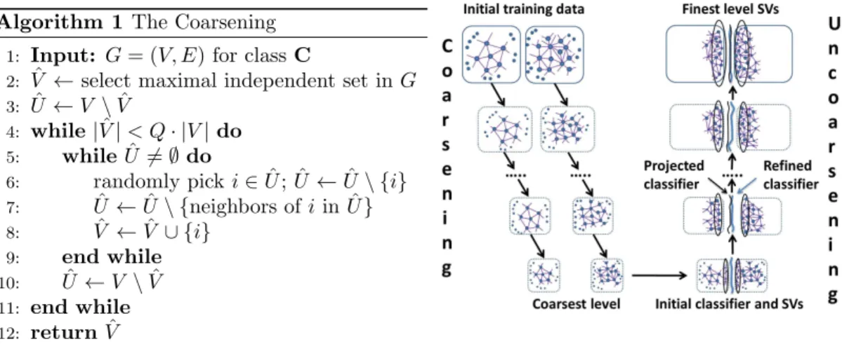
The proposed MF (see Figure 1) includes three phases: gradual training set coarsening, coars-est support vectors’ learning, and gradual support vectors’ refinement (uncoarsening). Separate coarsening hierarchies are created forC+, andC−independently. Each next-coarser level con-tains a subset of points of the corresponding fine level. These subsets are selected using the approximated k-nearest neighbor graphs (AkNN). In contrast to the coarsening used in mul-tilevel dimensionality reduction method [6], we found that selecting an independent set only does not lead to the best computational results. Instead, making the coarsening less aggressive makes the framework much more robust to the changes in the parameters. After the coarsest level is solved exactly, we gradually refine the support vectors and the corresponding classifiers.
The Coarsening Phase. The coarsening algorithms are the same for both C+, andC−, so we provide only one of them. Given a class of data points C, the coarsening begins with a construction of AkNN G= (V, E), whereV =C, andEare the edges of AkNN. The goal is to select a set of points ˆV for the next-coarser problem, where|Vˆ| ≥Q|V|(typicallyQ= 0.5). The second requirement for ˆV is that it has to be a dominating set ofV. The coarsening for classC
is presented in Algorithm 1. It consists of several iterations of independent set ofV selections that are complementary to already chosen sets. We begin with choosing a random independent set (l. 2) using greedy algorithm. It is eliminated from the graph, and the next independent set is added to ˆV (l. 5-9). For imbalanced cases, when WSVM is used, we avoid of creating very small coarse problems forC+. Instead, already very small class is continuously replicated across the rest of the hierarchy ifC− still requires coarsening. We note that this method of coarsening will reduce the degree of skewness in the data and make the data approximately balanced at the coarsest level. The multilevel framework recursively calls the coarsening process until it creates a hierarchy ofrcoarse representations{Ji}ri=0ofJ. At each level of this hierarchy, the
corresponding AkNNs’ {Gi = (Vi, Ei)}ri=0 are saved for future use at the uncoarsening phase.
Algorithm 1 The Coarsening
1: Input: G= (V, E) for classC
2: Vˆ ←select maximal independent set inG 3: Uˆ ←V \Vˆ 4: while|Vˆ|< Q· |V|do 5: whileUˆ =∅do 6: randomly pick i∈Uˆ; ˆU ←Uˆ\ {i} 7: Uˆ ←Uˆ \ {neighbors ofiin ˆU} 8: Vˆ ←Vˆ ∪ {i} 9: end while 10: Uˆ ←V \Vˆ 11: end while 12: returnVˆ
Figure 1: The MF for (W)SVM.
The Coarsest Problem. At the coarsest levelr, when |Jr|<< J, we can apply an exact
algorithm for training the coarsest classifier. Processing the coarsest level includes an applica-tion of the UD [3] model selecapplica-tion to get high-quality classifiers on the difficult data sets.
The Refinement Phase. Given the solution of coarse leveli+ 1 (the set of support vectors Si+1, and parameters Ci+1, and γi+1), the primary goal of the refinement is to update and
optimize this solution for the current fine leveli. Unlike many other multilevel algorithms, in which the inherited coarse solution contains projected variables only, we initially inherit not only the coarse support vectors but also parameters for model selection. This is because the model selection is an extremely time-consuming component of (W)SVM, and can be prohibitive at fine levels. However, at the coarse levels, when the problem is much smaller than the original, we can apply much heavier methods for model selection without any loss in the total complexity.
Algorithm 2 The Refinement at leveli 1: Input: Ji, Si+1, Ci+1, γi+1
2: if iis the coarsest level then
3: Calculate the best (Ci,γi) using UD
4: Si←Apply SVM onXi
5: end if
6: Calculate nearest neighborsNifor support
vectorsSi+1 from the existing AkNN Gi
7: data(traini) ←S(i+1)∪Ni 8: if |data(traini) |< Qdt then
9: CO←Ci+1;γO←γ i+1
10: Run UD using the center (CO, γO)
11: else
12: Ci ←Ci+1; γi←γi+1
13: end if
14: if |data(traini) | ≥Qdt then
15: Clusterdata(traini) into Kclusters 16: ∀k ∈ K find P nearest opposite-class
clusters
17: Si ← Apply SVM on pairs of nearest clusters only
18: else
19: Si←Apply SVM directly ondata(traini)
20: end if
21: ReturnSi,Ci,γi
The refinement is presented in Algorithm 2. The coarsest level is solved exactly and rein-forced by the model selection (l. 2-5). Ifiis one of the intermediate levels, we build the set of training datadata(traini) by inheriting the coarse support vectorsSi+1 and adding to them some
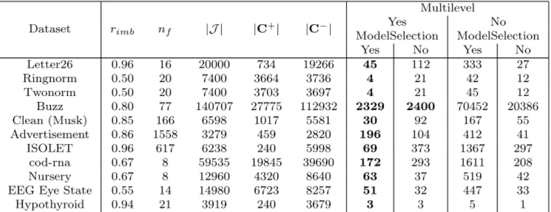
Table 1: Benchmark datasets and computational time (in sec.) of multilevel, and regular SVM. Dataset rimb nf |J | |C+| |C−| Multilevel Yes No ModelSelection ModelSelection Yes No Yes No Letter26 0.96 16 20000 734 19266 45 112 333 27 Ringnorm 0.50 20 7400 3664 3736 4 21 42 12 Twonorm 0.50 20 7400 3703 3697 4 21 45 12 Buzz 0.80 77 140707 27775 112932 2329 2400 70452 20386 Clean (Musk) 0.85 166 6598 1017 5581 30 92 167 55 Advertisement 0.86 1558 3279 459 2820 196 104 412 41 ISOLET 0.96 617 6238 240 5998 69 373 1367 297 cod-rna 0.67 8 59535 19845 39690 172 293 1611 208 Nursery 0.67 8 12960 4320 8640 63 37 519 42
EEG Eye State 0.55 14 14980 6723 8257 51 32 447 33
Hypothyroid 0.94 21 3919 240 3679 3 3 5 1
than 5). If the size of data(traini) is still small enough (relatively to the existing computational resources, and the initial size of the data) for applying model selection, and solving SVM on the wholedata(traini) , then we use coarse parametersCi+1, andγi+1 as initializers for the current
level, and retrain (l. 9-10,19). Otherwise, the coarseCi+1, andγi+1 are inherited inCi, andγi
(l. 12). Then, being large for direct application of the SVM, data(traini) is clustered into several
clusters, and pairs of nearest opposite clusters are retrained, and contribute their solutions to Si (l. 15-17). We note that cluster-based retraining can be done in parallel, as different pairs of
clusters are independent. Moreover, the total complexity of the algorithm does not suffer from reinforcing the cluster-based retraining with model selection.
3
Computational Results
Discussion and full results of our work can be found in [5]. The multilevel (W)SVM are evalu-ated on binary classification benchmarks from UCI repository. Single SVM and WSVM models are solved using LIBSVM-3.18 [2], and the AkNN graphs are costructed using FLANN library [4]. Multilevel frameworks are implemented in MATLAB 2012a, and evaluated on Linux. The results for multilevel (W)SVM (objectives and running times) should only be considered qual-itatively and can certainly be further improved by a more advanced implementation. The implementation is available at http://www.cs.clemson.edu/~isafro/software.html. Eval-uation of the proposed algorithm is done using accuracy (ACC), sensitivity (SN), specificity (SP), and the geometric mean of SN and SP (G-mean). The details of the datasets are de-scribed in left part of Table 1. We normalize all data prior to classification in order to get zero mean and unitary standard deviation. We perform a 9- and 5-point run design for the first and second stages of the nested UD.
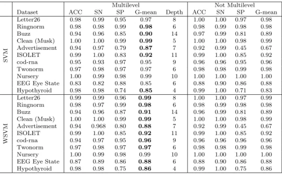
The performance measures of the multilevel (W)SVM (Table 2, left part of the table) are compared with the regular (one-level) (W)SVM (Table 2, right part of the table). Since sev-eral components in the coarsening, and uncoarsening schemes are randomized algorithms, the average numbers over 100 random runs are reported for each data set. We do not report the standard deviations because in all experiments they are negligibly small. Bold fonts emphasize the best G-mean results. Table 2 demonstrates that the quality of multilevel SVM algorithms is very similar to the quality of the single-level SVM. However, we observed that multilevel WSVM improves the single-level WSVM for some datasets.
The main achievement of the proposed multilevel scheme is its computational time (see Table 1) that substantially improves that of the single-level (W)SVM when the model selection techniques must be applied on difficult data sets. We note that for most of the datasets in the benchmark, using model selection was extremely important for obtaining high-quality results. Moreover, the observed improvement is not complete, because (similar to many multilevel and multigrid algorithms) the refinement phase can be easily parallelized at levels where the training by clusters is employed. In addition, the proposed methodology is very successful for large imbalanced classification problems since it can reduce the degree of skewness in the data and make the data approximately balanced at the coarse levels.
Table 2: Performance measures for multilevel and regular SVMs and WSVMs. Each cell con-tains an average over 100 executions. Column ’Depth’ shows the number of levels.
Multilevel Not Multilevel
Dataset ACC SN SP G-mean Depth ACC SN SP G-mean
SVM Letter26 0.98 0.99 0.95 0.97 8 1.00 1.00 0.97 0.98 Ringnorm 0.98 0.98 0.99 0.98 6 0.98 0.99 0.98 0.98 Buzz 0.94 0.96 0.85 0.90 14 0.97 0.99 0.81 0.89 Clean (Musk) 1.00 1.00 0.99 0.99 5 1.00 1.00 0.98 0.99 Advertisement 0.94 0.97 0.79 0.87 7 0.92 0.99 0.45 0.67 ISOLET 0.99 1.00 0.83 0.92 11 0.99 1.00 0.85 0.92 cod-rna 0.95 0.93 0.97 0.95 9 0.96 0.96 0.95 0.96 Twonorm 0.97 0.98 0.97 0.97 6 0.98 0.98 0.99 0.98 Nursery 1.00 0.99 0.98 0.99 10 1.00 1.00 1.00 1.00 EEG Eye State 0.83 0.82 0.88 0.85 6 0.88 0.90 0.86 0.88 Hypothyroid 0.98 0.98 0.74 0.85 4 0.99 1.00 0.71 0.83 WSVM Letter26 0.99 0.99 0.96 0.99 8 1.00 1.00 0.97 0.99 Ringnorm 0.98 0.97 0.99 0.98 6 0.98 0.99 0.98 0.98 Buzz 0.94 0.96 0.87 0.91 14 0.96 0.99 0.81 0.89 Clean (Musk) 1.00 1.00 0.99 0.99 5 1.00 1.00 0.98 0.99 Advertisement 0.94 0.968 0.80 0.88 7 0.92 0.99 0.45 0.67 ISOLET 0.99 1.00 0.85 0.92 11 0.99 1.00 0.85 0.92 cod-rna 0.94 0.97 0.95 0.96 9 0.96 0.96 0.96 0.96 Twonorm 0.97 0.98 0.97 0.97 6 0.98 0.98 0.99 0.98 Nursery 1.00 0.99 0.98 0.99 10 1.00 1.00 1.00 1.00 EEG Eye State 0.87 0.89 0.86 0.88 6 0.88 0.90 0.86 0.88 Hypothyroid 0.98 0.98 0.75 0.86 4 0.99 1.00 0.75 0.86
References
[1] A. Brandt and D. Ron. Chapter 1 : Multigrid solvers and multilevel optimization strategies. In J. Cong and J. R. Shinnerl, editors,Multilevel Optimization and VLSICAD. Kluwer, 2003. [2] Chih-Chung Chang and Chih-Jen Lin. Libsvm: a library for support vector machines. ACM
Transactions on Intelligent Systems and Technology (TIST), 2(3):27, 2011.
[3] C.M. Huang, Y.J. Lee, D.K.J. Lin, and S.Y. Huang. Model selection for support vector machines via uniform design. Computational Statistics & Data Analysis, 52(1):335–346, 2007.
[4] Marius Muja and David G. Lowe. Fast approximate nearest neighbors with automatic algorithm configuration. In International Conference on Computer Vision Theory and Application VISS-APP’09), pages 331–340. INSTICC Press, 2009.
[5] T. Razzaghi and I. Safro. Fast multilevel support vector machines. ArXiv, abs/1410.3348, 2014. [6] S. Sakellaridi, Haw ren Fang, and Y. Saad. Graph-based multilevel dimensionality reduction with
applications to eigenfaces and latent semantic indexing. In Machine Learning and Applications, 2008. ICMLA ’08. Seventh International Conference on, pages 194–200, Dec 2008.