Ring coupled-cluster doubles correction to geminal wavefunctions
´
A. Szabados and ´A. Marg´ocsy
Laboratory of Theoretical Chemistry, Lor´and E¨otv¨os University, H-1518 Budapest, POB 32, Hungary
ARTICLE HISTORY
Compiled February 28, 2017
ABSTRACT
A ring approximation in coupled cluster (CC) theory is worked out at the multi reference (MR) level. The underlying CC framework is based on generalized nor-mal ordering and applies the corresponding generalized Wick-theorem. Contrac-tions among cluster operators is avoided by adopting a normal ordered exponential Ansatz.
The MR ring CC doubles (MR rCCD) theory is found to represent a companion to the previously introduced extended random phase approximation (ERPA). Equa-tions for wavefunction parameters are derived in parallel and compared. Condition for the ground state consistent with ERPA is obtained. This paves the way towards comparison with the ERPA based correction to the Antisymmetrized Product of Strongly Orthogonal Geminal (APSG) reference, ERPA-APSG.
KEYWORDS
ring coupled-cluster doubles; multireference approach; generalized Wick theorem, random phase approximation; geminal wavefunction
1. Introduction
Coupled-cluster (CC) theory, based on a closed shell reference determinant is often relied on when highly accurate quantum chemical results are needed. While the CC parametrization of the wavefunction is in principle exact in the given basis, cutting off the cluster operator is necessary for practical application. Truncation of the cluster op-erator unfortunately undermines the performance of single reference (SR) CC theory when the so-called static correlation involves determinants beyond the excitation level included inT. Such situations call for extension of the original theory e.g. by modifying the amplitude equations[1] or by abandoning the idea of a single, closed shell reference. The latter route has been extensively investigated by professor Debashis Mukherjee throughout his career, starting with open-shell CC formulations[2, 3], followed by ideas based on the eigenvalue independent partitioning[4, 5] or those exploiting the Jeziorski-Monkhorst[6] parametrization of the wavefunction[7]. An extremely simple version of multireference (MR) CC theory was put forward by Mukherjee and coworkers[8, 9], inspired by the idea of generalizing the concept of normal ordering for a multideter-minantal reference function[10, 11] It is the internally contracted MR CC formulation of Ref.[8] that provides the starting point of the present work.
Our focus is now put on the so called ring approximation of the CC doubles equa-tions (rCCD), introduced in the quantum chemical context probably by Ciˇzek[12]. Sin-gle reference rCCD theory represents a kind of crossroads of approximation strategies for the molecular electronic structure problem. When formulated with spin-orbitals, equations of the random phase approximation (RPA) can be cast in a form matching the rCCD equations and the rCCD wavefunction can be regarded the ground state consistent with RPA excited states.[13, 14, 15] Admitting several variants, RPA can be derived in the framework of polarization propagator theory[16], it can be obtained in the context of time-dependent (TD) density functional theory (DFT)[17], by com-bining the adiabatic connection idea with the fluctuation-dissipation theorem within DFT[18, 17] or based on Green-function theory.[19] Note, that RPA is understood presently as particle-hole RPA, no consideration of the particle-particle extension is made here.[20, 21]
The ring approximation of CCD is certainly not free from the problems of trun-cated CC theory mentioned above. As a simple amendment, exchange counterparts of the antisymmetrized integrals can be deleted, leading to the direct rCCD (drCCD) method. The performance of drCCD together with several exchange corrected RPA variants was evaluated by Klopper et al.[22].
When wishing to make rCCD applicable for inherently MR situations, it appears plausible to approach from the multideterminantal reference perspective. Given the various facets of the single reference theory, remarkably diverse routes are provided for a MR extension. Of these possibilities, the RPA approach was picked in several instances. Oddershede, e.g. gave a multireference RPA formulation within the prop-agator context[16]. Pernal worked out an extended RPA (ERPA) for the multirefer-ence situation[23] based on Rowe’s equation-of-motion theory[24] for obtaining excited states. Pernal also developped a theory for obtaining a correction to the ground state reference energy based on the solution of the ERPA equations[25, 26].
The present study adds to the picture by exploring the CC aspect in the MR sit-uation. Our goal on one hand is to examine the MR extension of the formal relation between rCCD, RPA and its consistent ground state. A further motivation is provided by our long term interest in applying the antisymmetrised product of strongly orthog-onal geminal (APSG) function[27, 28] as a mulideterminantal reference for electron correlation treatment. While a recent study, based on linearized CC, called attention to an inherent failure of the APSG function in the multiple bond breaking situation[29], the success of ERPA-APSG hints that a ring approximation of CC might overcome this problem.
The MR CC method considered here is based on generalized normal ordering (GNO) and applies the corresponding generalized Wick’s theorem (GWT)[9, 10, 11, 30, 31]. Double excitations entering the cluster operator have a general flavour. Contractions among terms of the cluster operator are avoided by assuming a normal ordered ex-ponential Ansatz, suggested by Lindgren[32]. We take an antisymmetrised product of strongly orthogonal geminal (APSG) function[27] as reference and tailor the theory to be as parallel as possible with the existing ERPA-APSG method of Pernal. This is the reason for picking the original rather than the improved version[9] of the underlying CC theory.
In what follows the MR rCCD theory is outlined first, giving explicit formulae within the approximations introduced. A companion RPA theory is presented next and found to agree with Pernal’s ERPA equations. The Riccati form of the ERPA equations are contrasted then with the MR rCCD equations. Finally, a set of approximate consis-tency conditions are derived for ERPA.
Let us note here, that the ring approximation of SR CCD is not invariant to the way the cluster operator is parametrized, see e.g. the Appendix of Ref.[33]. Equivalence of RPA and rCCD equations as well as strict matching with the consistent ground state of RPA implies a spin-orbital based, closed shell formulation. We work with spin-free operators presently and give the respective relations at the SR level in Appendix.
2. Preliminaries
We consider an APSG function[27], denoted by |0⟩, and assume that orthonormal orbitals indexed by p, q, . . . are natural orbitals of |0⟩. An APSG function is built of two-electron fragments (geminals), each fragment being expanded over a mutually exclusive set of natural orbitals (termed geminal subspaces). The second quantized expression of APSG reads
|0⟩ = N/2∏ I=1 ∑ p∈I cpa+pβa+pα|vac⟩ , (1)
whereN stands for the number of electrons andI refers to the geminal subspace. From Eq.(1) it is apparent, that APSG is expanded in the seniority zero subspace[34] of the Hilbert space. In the case where each geminal subspace is two dimensional, APSG agrees with the generalized valence bond function.
In terms of coefficientscp, diagonals of the spin-dependent density matrix are given
as
np = ⟨0|a+pσapσ|0⟩ = c 2
p . (2)
The corresponding hole density matrix element is denoted by overline:
np = 1−np .
Besides 1-body density matrices, 2-body reduced density matrix elements will be in-volved in the following development. For completeness, we give here the expression of the 2-body cumulant of APSG, defined as
λrσsσ′ pσqσ′ = ⟨0|a + rσa + sσ′aqσ′apσ|0⟩ − δprδqsnpnq + δσσ′δpsδqrnpnq .
Summing for both spin indices of the above spin-dependent cumulant one obtains
Λrspq = ∑
σσ′ λrσsσ′
pσqσ′ = 2δIrIsnrns(δpsδqr − 2δprδqs) + 2δIpIrcpcrδpqδrs . (3)
In the above, Ir denotes that geminal subspace which accommodates natural orbital
r.
A GNO, denoted by{.} will be used below, satisfying the condition
⟨0|{.}|0⟩ = 0 . (4)
A second quantized string of operators in GNO involves particle and hole density matrices as well as cumulants of the reference function, as described by Kutzelnigg and
Mukherjee[11] and proved by Kong, Nooijen and Mukherjee[31]. The normal ordered form of the electronic Hamiltonian accordingly reads
H = E0 + ∑ pq fqp {Epq} | {z } {H1} + 1 2 ∑ pqrs vrspq {Epqrs} | {z } {H2} (5)
with the APSG reference energy being
E0 = ⟨0|H|0⟩,
the spin-summed single excitation operator defined as
Epr = ∑
σ
a+rσapσ , (6)
and the doubly exciting, spin-summed operator taking the form
Erspq = EprEqs .
The two-electron integral in⟨12|12⟩ convention is expressed as vrspq =⟨rs|pq⟩ and the
Fockian entering Eq.(5) reads
fqp = hpq + ∑
r vprqrnr
where
vprqr = 2vqrpr−vprrq .
3. Ring CCD based on APSG
With the aim of correcting APSG by CC, a cluster operator involving solely double excitations is written as T2 = 1 2 ∑ p<r q<s tpqrs {Epqrs}. (7)
In the above and throughout index restrictionp < r is used as a shorthand for np ≥ nr, p ̸= r. (Note, that assuming orbitals ordered in decreasing occupation number,
r < pis still possible if np =nr. The case of np =nr is allowed only for non integer
occupation numbers. Bothnp =nr = 0 and np =nr = 1 are excluded.) Amplitudes
tpqrsexhibit the single symmetry relationtpqrs =tsrqp. Amplitudestpqrsandtqprsare unrelated
whenr ̸=sand p̸=q.
A normal ordered exponential Ansatz is taken for the corrected wavefunction
satisfying the intermediate normalization condition
⟨0|Ψ⟩ = 0
by virtue of definition (4) of GNO. Energy E corresponding to Ψ is conveniently written as
E = E0 + ∆E . (9)
Substituting Eqs.(5), (7), (8) and (9) in the Schr¨odinger equation
H Ψ = E Ψ (10)
and projecting from the left by⟨0|results in the energy correction
∆E = ⟨0|{H2}{T2}|0⟩ . (11)
To obtain the amplitude equations, Eq.(10) is projected from the left by the doubly excited functions ⟨0|{Evuyx}† = ⟨0|{Exyuv} , u < x, v < y . (12) This results ⟨0|{Exyuv}{H2}|0⟩ + ⟨0|{Exyuv}({H1}+{H2}){T2}|0⟩ + 1 2⟨0|{E uv xy}{H2}{T22}|0⟩′ = 0 , (13)
where the prime on the last term on the lhs of Eq.(13) indicates omission of contraction patterns producing ∆E, i.e. where{H2}is contracted completely with one of theT2’s. Up to this point the derivation followed SR CCD theory[35, 36] closely. Index restric-tions, e.g. in Eq.(7) taking the place of occupied/virtual categorization and {expT2}
standing in Eq.(8) instead of exp{T2} are the only notable deviations. A marked
dif-ference with SR theory appears when expectation values in Eqs.(11) and (13) are evaluated based on the GNO and the associated GWT. With ordinary normal order-ing, pair contractions (i.e. rank-1 contractions) appear solely in expectation values with the reference. In the general situation contractions up to rank-k appear when calculating the expectation value of a string composed of 2k operators. The geminal structure of the reference represents an advantage at this point. Due to the fact, that 3-body or higher cumulants (up toN) are explicitly zero with a geminal reference, at most rank-2 contractions appear in our case.1 Even by this, the number of patterns
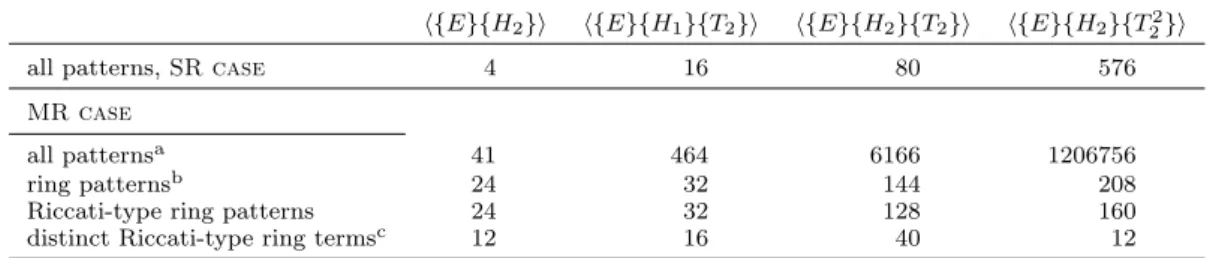
obtained by the GWT is huge, as reflected in the second row of Table 1. The SR case is shown for comparison in the first row. The couple of hundred terms of the SR case are usually dealt with by diagram techniques. Diagrammatics in the context of GNO and GWT was initiated by Kutzelnigg and Mukherjee[11], it is however less used. When relying on the GWT, contraction patterns are most often generated and processed by computer.[38, 39] We adopt the latter practice, utilizing a code written in our laboratory in PYTHON language.
1It is interesting to observe that (N+1)-body and higher cumulants become nonzero even if the corresponding
Table 1. Number of contraction patterns, obtained by the GWT, contributing to the terms of the CCD equations, Eq.(13). Cumulants of order (N+ 1) or higher are omitted,N denoting the number of electrons.
⟨{E}{H2}⟩ ⟨{E}{H1}{T2}⟩ ⟨{E}{H2}{T2}⟩ ⟨{E}{H2}{T22}⟩
all patterns,SR case 4 16 80 576
MR case
all patternsa 41 464 6166 1206756
ring patternsb 24 32 144 208
Riccati-type ring patterns 24 32 128 160 distinct Riccati-type ring termsc 12 16 40 12 a Germinal structure of the reference is assumed.
bProducts of 2-body cumulants are omitted.
cSimplifications exploit integral, amplitude and cumulant symmetries and exchange of equivalent indices.
We presently do not aim at generating and implementing all terms at the MR CCD level. We rather wish to devise the simplest approximation to arrive at a MR rCCD theory paralleling the existing APSG based ERPA. First of all, terms at most linear in cumulants are kept only, since powers of cumulants do not appear in ERPA-APSG theory. Dropping terms including products of cumulants could be rationalized on the basis that their first power is already negligible. Unfortunately this argument is not always supported numerically.[40] This step is consequently better understood as a first approximation that may need rectification later.
As a second approximation, non-ring contraction patterns are neglected. Identifi-cation of ring patterns is performed based on the algebraic expression. In short, we consider a contraction pattern of ring type, if index pairs subject to the constraint introduced in Eq.(7) (e.g. p < r) can be introduced as hyper indices and the term can be recast as product of matrices, indexed by these hyper indices. There are some subtleties to this definition that are best conveyed by sketching the algorithm devised for the analysis. Let us consider a contraction pattern multiplied with the appro-priate tensor elements (i.e. f, v and t) according to Eq.(13). Summation is implied, indices not involved in summation are regarded outer. Among summation indices, constrained (originating fromT) and unconstrained (originating fromH) indices are distinguished. Prior to ring analysis, hyper indices (i.e. indices related by inequal-ity) are established. We then go through the following steps, starting with the first contraction pattern
(1) reduce the number of summation indices by evaluating Kronecker-deltas implied by rank-1 contractions; favour constrained indices over unconstrained ones; (2) if there are unconstrained summation indices still left, establish the tensor
ele-ments (i.e.f,v orλ) they connect; tensor elements multiplied then summed for common, unconstrained indices are considered hyper tensors;
(3) initialize logical variable ring as ‘true’;
(4) take each hyper index formed of outer indices and determine whether the con-tributing orbital indices occur on the same tensor (i.e. f, v, λ or t) or hyper tensor; if they occur ont, they even have to be arranged vertically; if any of this fails setring ‘false’
(5) if ringis ‘true’, goto 7
(6) if the expression is linear inT and three of the outer indices occur ontand one hyper index can be formed ontvertically, the diagonal part of the hyper tensor is kept; otherwise the term is dropped; goto 9
indices occur on the same tensor (i.e.f,v,λort) or hyper tensor; if they occur ont, they even have to be arranged vertically; if any of this fails setring‘false’; (8) if ringis ‘true’, the term is kept, otherwise dropped;
(9) proceed to next contraction pattern and goto 1
When performed at the SR level, the above algorithm properly generates the ring CCD equations.
Let us consider some examples to illustrate the steps of ring filtering. Take e.g. the following two terms contributing to⟨0|{Exyuv}{H1}{T2}|0⟩,u < x, v < y:
−nunvnx ∑ qr q<x,u<r αvryqtuqrx (14) nunvnx ∑ q<s αvsyqtuqxs (15)
with the hyper tensor element
αvryq = ∑
t
ftvΛtryq .
The term in Eq.(14) is dropped at point 4, since outer indicesuandx, forming a hyper index, occur crosswise on amplitude t. The term of Eq.(15) is kept at point 4, since both index pairsuxandvyconform to the requirements. The expression of Eq.(15) is approved at point 7 also, where hyper indexqsis examined. It eventually contributes a term in the second row of the expression ofACC, given in Appendix B.
An example for the diagonal term under point 6, is given by the following expression, contributing to⟨0|{Exyuv}{H2}{T2}|0⟩,u < x, v < y: nunvnxny ∑ r u<r βrxtuvry (16)
with the hyper tensor element
βxr = ∑
pqs
vxspqΛsrpq .
When making the ring approximation,r ̸=xterms of the sum in Eq.(16) are dropped. Ther =x term contributes a term in the last row of the expression ofACC, given in Appendix B.
As a final example consider the following term contributing to
⟨0|{Exyuv}{H2}{T22}|0⟩,u < x, v < y: −nunx∑ p<r q<s t<w npnqnsnwvswpq Λvryttpqrsttuwx .
This is dropped at point 7 of the ring filtering as hyper indexpr is broken up, p and
r occurring separately on tensors v and Λ . The same hold fortw.
Eliminating non-ring terms reduces the number of contraction patterns consider-ably, as reflected in the third row of Table 1. One further trimming is still to be
performed though. It turns out that not all terms admitted by the ring approximation conform with the algebraic Riccati equation derived from RPA equations. An example is provided by the following expression, again contributing to⟨0|{Exyuv}{H2}{T2}|0⟩:
nvny ∑ p<r q<s
Λurxp tpqrs nqnsvqysv .
A characteristic feature of the term above is that tensor elements Λ andvare connected via t. When introducing hyper indices, the corresponding term involves two matrix factors multiplying t, yielding an expression likeΛtw (with wqs,vy =nqnsvqysv). This
and similar terms are dropped presently as they can not be accommodated in the Riccati equation we wish to obtain. The remaining number of contraction patterns and the number of distinct terms upon performing simplifications are indicated in the last two rows of Table 1.
Adopting matrix notation, the final form of the Riccati-type ring amplitude equation is obtained as
BCC + 2ATCCt + 2t ACC + 4t M BCCM t = 0 (17)
withtpr,qs=tpqrs and subscript CC labeling matrix factors originating from the rCCD
equations. Diagonal matrix M is built of occupation numbers as
Mpr,qs = δpqδrsnpnr . (18)
Elements of matricesACC andBCCare given in Appendix B.
Amplitudes obtained from Eq.(17) are substituted in Eq.(11) to yield the MR rCCD energy correction, reading as
∆ErCCD = Tr (M BCCM t) , (19)
neglecting terms including products of cumulants.
4. Extended RPA based on APSG
In the framework of equation of motion theory[24] an excitation operator of the com-panion RPA to the ring CCD of the previous Section is written as
O†ω = ∑ p<r ( Xprω {Epr} − Yprω {Erp}) . (20) Regarding that {Epr} = Epr − δprnp
and that p = r is excluded, the excitation operator of Eq.(20) agrees with that of extended RPA, c.f. Eq.(21) of Ref.[25]. Equations of ERPA determining excited state
coefficientsXprω, Yprω and excitation energiesω are concisely written as ( A B −B −A ) ( X Y ) = ( S 0 0 S ) ( X Y ) ωERPA (21) with Aqs,pr = ⟨0|[Esq,[H, Epr]]|0⟩/2 Bqs,pr = − ⟨0|[Esq,[H, Erp]]|0⟩/2 Sqs,pr = ⟨0| [ Esq, Erp]|0⟩/2
andω being the column index in matricesX andY . Diagonal matrixωERPAinvolves only the physically relevant, positive roots. (Factor 1/2 in the above definition of matrices A, B and S is introduced to agree with the expressions of Ref.[26]. The reversed sign of B originates in the reversed sign of Yprω in Eq.(20), compared with Ref.[25]. )
The overlap matrix on the rhs of Eq.(21) is diagonal, reading as
Sqs,pr = δqpδsr(np−nr) .
It is easy to see based on Eq.(2) thatS can be decomposed as
S = KL
withKqs,pr = δqpδsr(cp+cr) andLqs,pr = δqpδsr(cp−cr) . Supposing that cp+cr
andcp−cr are nonzero for allp, r, Eq.(21) can be rewritten as ( A−+ B−− −B++ −A+− ) ( KX LY ) = ( KX LY ) ωERPA (22) with A−+ = L−1AK−1 A+− = K−1AK−1 B−− = L−1BL−1 B++ = K−1BK−1 .
The Riccati-type equation associated with the ERPA equations can now be obtained by (i) multiplying the first equation in Eq.(22) by (KX)−1from the right; (ii) multiplying the second equation in Eq.(22) by (KX)−1 from the right and left and subtracting the latter from the former. This yields
B++ + A+−CR + CRA−+ + CRB−−CR = 0 (23)
with
subscript R referring to the Riccati equation. When KX is invertible, Eq.(23) is equivalent[41] with the ERPA equation of Eq.(21). Introduction of matrix factorsK andLhere is not completely coherent with Pernal[23], but it does not affect the essen-tial equivalence with Eq.(21). Expression of matrix factorsA+−,A−+ and B++/−− is given in Appendix C to assist the comparison of the rCCD rooted Riccati equa-tion Eq.(17) with Eq.(23), originating from ERPA. Note, that these equaequa-tions are not exactly the same already at the SR level, there appears a factor of two between the solutions, c.f. Eq.(A10) of Appendix A. At the MR level the deviation is increased. While the SR limiting case of matrix factors in Eqs.(17) and (23) matches, the cu-mulant involving terms do not lend themselves to setting an explicit relation. An important difference concerns symmetry conservation of an initial guess during the it-erative solution of Eqs.(17) and (23). Due to the appearance ofACC and its transpose in the linear terms and due toBCC being symmetric, symmetry of an initial t is not destroyed by the ring CCD equation.2 In the case of Eq.(23), symmetry of CR is not
ensured as B is not symmetric and A−+ ̸= (A+−)T. A further difference between
Eqs.(17) and (23) may be worth to note here. Matrices K or L becoming singular is a problem with Eq.(23), a caveat oncp ±cr getting close to zero has been in fact
mentioned.[26] The Riccati equation in Eq.(17) could run into a similar problem if particle and hole occupation numbers appearing under the inverse in the expression of ACC and BCC became zero. This is however excluded by the restriction imposed on indices in Eq.(7) and Eq.(12).
It is possible to deduce an energy expression from the first equation of Eq.(22) by multiplying again from the right by (KX)−1 and performing a trace. This, so-called plasmon formula reads
∆Eplasmon = 1 2Tr(ω ERPA− A−+) = 1 2Tr(B −−C R) . (25)
This expression could be compared to the MR rCCD energy correction Eq.(19) were the relation betweenCRandtknown. At the SR level ∆Eplasmonagrees with ∆ErCCD,
c.f. Eq.(A19). This is the reason behind introducing the factor 1/2 in Eq.(25). To assist comparison between the SR and MR case, quantities introduced during the derivation and their relation are summarized in Tables 2 and 3and , respectively. At difference with the SR situation, there appears no obvious formal correspondence between the solutions of the Riccati equations Eq.(17)) and Eq.(23). For this reason a numerical comparison is called for contrasting the above ∆Eplasmon with ∆ErCCD at the MR
level.
5. Ground state consistent with ERPA
Though Eq.(25) could be considered an ERPA energy correction formula, the analo-gous expression at the SR level (c.f Eqs.(A17) and (A18)) does not match the energy correction of the consistent ground state (c.f. Eq.(A16)) and the latter is preferred to the former in such a case.[42, 43] Motivated by this, we parametrize a ground state in
the ERPA framework as |Φ⟩ = exp( 1 2 ∑ p<r q<s τrspq {Epqrs}) |0⟩
and seek an expression for amplitudesτ from the consistency condition
Oω|Φ⟩ = 0.
SubstitutingOω from Eq.(20) we obtain ∑ u<x (Xuxω {Exu} − Yuxω{Eux})|0⟩ + 1 2 ∑ u<x p<r,q<s τrspq(Xuxω {Exu} − Yuxω{Eux}){Epqrs}|0⟩ = 0.
Applying GWT, the second term on the lhs can be written as a sum of normal ordered products. Terms of the resulting expression can be identified as genuine 3-body, 2-body etc. excitations out of APSG. In analogy with the SR treatment, at most single excitations are retained as a first approximation. A further simplification is introduced by neglecting terms involving cumulants of APSG. Among others, this latter step wipes all terms involving the unexcited APSG function, leading to
0 = ∑ u<x (Xuxω {Exu} − Yuxω{Eux})|0⟩ + 1 2 ∑ u<x p<r,q<s τrspqXuxω ( 2δupδxrnpnr{Esq}+2δuqδxsnqns{Epr}−δupδxsnpns{Eqr}−δuqδxrnqnr{Eps} ) |0⟩ − 1 2 ∑ u<x p<r,q<s τrspqYuxω (
2δurδxpnpnr{Esq}+2δusδxqnqns{Epr}−δusδxpnpns{Eqr}−δurδxqnqnr{Eps})|0⟩ Index restrictions disclose the first two terms in the parenthesis multiplyingYuxω . Fur-thermore, we have to distinguish cases in the third and fourth term of the parenthesis multiplying Xuxω , namely q < r, q = r, r < q and p < s, p = s, s < p respectively3.
3For simplicity, an ordering in decreasing order ofn
pis assumed in this section andp < sis to be understood
Upon simplifications, we are lead to 0 = ∑ p<s q npnsτqspqXpsω {Eqq}|0⟩ (26) + ∑ p<r ( Xprω − ∑ q<s nqnsτpsqrXqsω ) {Erp}|0⟩ + ∑ p<r ( −Yprω + ∑ q<s nqns(2τsrqp−τrsqp)Xqsω + ∑ q<s nsnqτrqspYqsω ) {Epr}|0⟩ .
Note, that in the interest of transparency some index restrictions implied by am-plitudes, are not indicated. These are q < p , r < s in the second row above, and
p < q , s < r in the last term of the third row. One can proceed now by setting the terms of Eq.(26) zero individually. (This is consistent with requiring all projections with ⟨0|{Eux} vanish, and neglecting the cumulant arising from e.g. ⟨0|{Exu}{Epr}|0⟩ here also.)
From the first row of Eq.(26) it then follows that spectator amplitudes are zero:
τqspq = 0 , ∀p < s ,∀q .
From the second row, amplitudes with the following particular ordering of indices are zeroed
τpsqr = 0 , ∀q < p < r < s . (27) Using symmetry of the amplitude matrixτ, it follows from Eq.(27) that
τrqsp = 0 , ∀p < q < s < r
can be substituted in the third term of the third row of Eq.(26). A third consistency condition on the amplitudes is obtained consequently as
∑ q<s
nqns(2τsrqp−τrsqp)Xqsω = Yprω .
Introducing
(Cc)pqrs = 2τrspq−τsrpq , ∀p, q < r, s (28) matrixCc stemming from the consistency condition can be written as
Cc = Y X−1M−1 , (29)
admittingp < r pairs for whichnpnr is nonzero and assuming the existence ofX−1.
Note, that Eq.(29) determines only those elements of Cc, where the indices conform
with the restriction in Eq.(28). All other elements ofCc as well as the related
ampli-tudesτ are zero.
of the round bracket in the second row of Eq.(26) can not be eliminated within the approximations introduced. To get a refined picture, cumulants should be admitted in the consistency considerations.
For the time being we remain at the simplest level and observe the analogy of Eqs.(28) and (29) with their SR counterpart Eqs.(A15) and (Eq.(A8)). The expressions agree but for the diagonal matrix factor M−1 and the index restriction in Eq.(28) taking the place of occupied/virtual categorization. It is also interesting to notice, thatCRof Eq.(24), stemming fom the Riccati equation is not completely the same as
Cc originating from the consistency condition. They differ not only by matrix factors
built of occupation numbers but also in the number of zero entries. The latter follows from index restriction of Eq.(28) affectingCc but notCR.
Deducing amplitudesτ from Cc as τrspq = 1
3
(
2 (Cc)pqrs + (Cc)pqsr )
an energy of the consistent ground state with ERPA can be obtained by substituting
τ in the MR CCD energy formula of Eq.(19). Numerical comparison of this MR CCD energy expression with the plasmon formula of Eq.(25) would be desirable. For this end, implementation by computer based code generation is currently in progress in our laboratory.
6. Conclusion
The formulae worked out above set the previously designed ERPA into a CC context at the MR level. Rather loose approximations are introduced in the CC derivation to achieve close correspondence with SR expressions and allow for transparent comparison with ERPA. Neglect of cumulants altogether when obtaining a consistent ground state for ERPA appears to be the least justified approximation. Omission of powers of cumulants when deriving the ring equations is also to be tested numerically.
Explicit expressions are obtained at the MR level for the rCCD energy, the plasmon formula as well as the energy of the ground state consistent with ERPA. Tables 2 and 3 summarize in a concise manner the quantities introduced at the SR and MR level, respectively. Matching of the RPA and rCCD rooted Riccati equations allows to draw a formal relation between the energy expressions collected in Table 2. At the MR level there appears no simple relation between matrix factors of the rCCD and ERPA rooted Riccati equations. For this reason a numerical comparison of the correlation energies will be necessary, with the ERPA-APSG energy formula[26] included as a fourth option.
The CC and ERPA formulae derived are general in the sense that explicit use of the reference being an APSG function was not made. It has to be kept in mind however, that omission of 3-body and higher cumulants (up to the number of electrons) follows from the geminal structure while it has to be regarded as an approximation for a non geminal reference. Taking APSG as reference is expected to have a beneficial effect on computational cost also, as all terms of the APSG cumulant is factorizable for Kronecker deltas, c.f. Eq.(3). The formal scaling of SR rCCD theory is therefore expected to persist, the MR extension affecting only the prefactor.
Let us comment finally on the superficial simplicity of the MR CC framework adopted here. As it was already alluded to, it has to be recognized that an enormous
Table 2. Quantities introduced in a spin-free formulation of RPA and rCCD, based on the HF determinant. Matrix factors of the Riccati equation are given in Eqs.(A5) and (A6). See Eq.(A8) for the relation betweenC andX,Y, Eq.(A10) gives the relation between C and t and finally Eq.(A15) shows the relation betweenC and τ. For the relation of the energy expressions, see Eqs.(A17), (A18) and (A19). In particular ∆Eplasmon= ∆ErCCD.
RPA for excited states normal RPA for the ground state ring CCD amplitudes of excited states X,Y Cii) n.a.i)
amplitudes of the ground state n.a. τ t
matrix factors of the Riccati equation A,B n.a. A,B
solution of the Riccati equation C n.a. C
correlation energy of the ground state ∆Eplasmon ∆ERPA ∆ErCCD i) n.a.: not applicable
ii)A quantity derived from the amplitudes of excited states.
Table 3. Quantities introduced in a spin-free formulation of RPA and rCCD, based on a multideterminantal reference. Matrix factors of the Riccati equations are given Appendices B and C. See Eq.(24) for the relation betweenCRand X,Y, Eq.(29) gives the relation betweenCcandX,Y and finally Eq.(28) shows the relation betweenCcandτ.
RPA for excited states normal RPA for the ground state ring CCD amplitudes of excited states X,Y Ccii) n.a.i)
amplitudes of the ground state n.a. τ t
matrix factors of the Riccati equation A−+/+−,B++/−− n.a. A CC,BCC
solution of the Riccati equation CR n.a. 2t
correlation energy of the ground state ∆Eplasmon ∆ERPA ∆ErCCD i)n.a.: not applicable
ii)A quantity derived from the amplitudes of excited states.
number of terms are generated by the GWT. In addition, there appears a redundancy among excited functions in the general case that has to be dealt with.[9] Redundancy is avoided here by resorting to double excitations in the cluster amplitudes. Extensiv-ity is always an issue to consider, especially for a CC theory. While the expressions reported above appear connected at first glance, spin cumulants represent a non trivial problem[44, 45] and for this reason the analysis is put off to further study.
Acknowledgement(s)
Discussions with prof. P.R. Surj´an (Budapest) are gratefully acknowledged.
Funding
The work has been supported by the National Research, Development and Innovation Office (NKFIH), under grant number K115744. One of the authors ( ´A.Sz.) acknowl-edges support by the J´anos Bolyai Research Scholarship of the Hungarian Academy of Sciences.
References
[1] K. Kowalski, P.D. Fan and P. Piecuch, Mol. Phys.103, 2191–2213 (2005). [2] I. Lindgren and D. Mukherjee, Physics Reports151, 93 – 127 (1987). [3] D. Mukherjee and S. Pal, Adv. Quantum Chem. 20, 291–373 (1989).
[4] D. Sinha, S.K. Mukhopadhyay, R. Chaudhuri and D. Mukherjee, Chem. Phys. Letters 154, 544 (1989).
[5] R. Chaudhuri, D. Mukhopadhyay and D. Mukherjee, Chem. Phys. Letters 162, 393–398 (1989).
[6] B. Jeziorski and H.J. Monkhorst, Phys. Rev. A24, 1668 (1981).
[7] U. Mahapatra, B. Datta and D. Mukherjee, J. Chem. Phys. 110, 6171–6188 (1999).
[8] U.S. Mahapatra, B. Datta, B. Bandyopadhyay and D. Mukherjee, in , Advances in Quantum Chemistry, Vol. 30, pp. 163 – 193.
[9] D. Sinha, R. Maitra and D. Mukherjee, Computational and Theoretical Chemistry
1003, 62 – 70 (2013).
[10] D. Mukherjee, Chemical Physics Letters274, 561 – 566 (1997).
[11] W. Kutzelnigg and D. Mukherjee, The Journal of Chemical Physics107, 432–449 (1997).
[12] J. ˇC´ıˇzek, J. Chem. Phys.45, 4256 (1966).
[13] N. Ostlund and M. Karplus, Chemical Physics Letters11, 450 – 453 (1971). [14] A.E. Hansen and T.D. Bouman, Molecular Physics37, 1713–1724 (1979). [15] G.E. Scuseria, T.M. Henderson and D.C. Sorensen, The Journal of Chemical
Physics 129, 231101 (2008).
[16] J. Oddershede, inAdvances in Chemical Physics (John Wiley & Sons, Inc., New York, 1987), Vol. 69, pp. 201–239.
[17] H. Eshuis, J.E. Bates and F. Furche, Theoretical Chemistry Accounts131, 1084 (2012).
[18] G. Jansen, R.F. Liu and J.G. ´Angy´an, The Journal of Chemical Physics 133, 154106 (2010).
[19] X. Ren, P. Rinke, C. Joas and M. Scheffler, Journal of Materials Science 47, 7447–7471 (2012).
[20] D. Peng, S.N. Steinmann, H. van Aggelen and W. Yang, The Journal of Chemical Physics 139, 104112 (2013).
[21] G.E. Scuseria, T.M. Henderson and I.W. Bulik, The Journal of Chemical Physics
139, 104113 (2013).
[22] W. Klopper, A.M. Teale, S. Coriani, T.B. Pedersen and T. Helgaker, Chemical Physics Letters 510, 147 – 153 (2011).
[23] K. Chatterjee and K. Pernal, The Journal of Chemical Physics 137, 204109 (2012).
[24] D. Rowe, Rev. Mod. Phys40, 153 (1968).
[25] K. Pernal, Journal of Chemical Theory and Computation10, 4332–4341 (2014). [26] E. Pastorczak and K. Pernal, Phys. Chem. Chem. Phys.17, 8622–8626 (2015). [27] P.R. Surj´an, Topics in Current Chemistry 203, 63–88 (1999).
[28] P. Jeszenszki, P.R. Nagy, T. Zoboki, ´A, Szabados and P.R. Surj´an, Int. J. Quan-tum Chem. 114, 1048 (2014).
[29] P.R. Surj´an, P. Jeszenszki and ´A. Szabados, Molecular Physics 113, 2960–2963 (2015).
[30] W. Kutzelnigg, K. Shamasundar and D. Mukherjee, Molecular Physics108, 433– 451 (2010).
[31] L. Kong, M. Nooijen and D. Mukherjee, The Journal of Chemical Physics 132, 234107 (2010).
[32] I. Lindgren, International Journal of Quantum Chemistry14, 33–58 (1978). [33] J. Toulouse, W. Zhu, A. Savin, G. Jansen and J.G. ´Angy´an, The Journal of
Chemical Physics 135, 084119 (2011).
[34] L. Bytautas, T.M. Henderson, C.A. Jim´enez-Hoyos, J.K. Ellis and G.E. Scuseria, The Journal of Chemical Physics135, 044119 (2011).
[35] I. Shavitt and R.J. Bartlett,Many-Body Methods in Chemistry and Physics (Cam-bridge University Press, Cam(Cam-bridge, 2009).
[36] G. E. Scuseria and C. L. Janssen and H. F. Schaefer, J. Chem. Phys. 89, 7382 (1988).
[37] M. Hanauer and A. K¨ohn, Chemical Physics401, 50 – 61 (2012), Recent advances in electron correlation methods and applications.
[38] R. Maitra, D. Sinha and D. Mukherjee, The Journal of Chemical Physics 137, 024105 (2012).
[39] L. Kong, K.R. Shamasundar, O. Demel and M. Nooijen, The Journal of Chemical Physics 130, 114101 (2009).
[40] J.M. Herbert, International Journal of Quantum Chemistry107, 703–711 (2007). [41] K. Zhou, J.C. Doyle and K. Glover,Robust and Optimal Control (Prentice-Hall,
Inc., Upper Saddle River, NJ, USA, 1996).
[42] T.I. Shibuya and V. McKoy, Phys. Rev. A2, 2208–2218 (1970).
[43] A. Szabo and N.S. Ostlund, The Journal of Chemical Physics 67, 4351–4360 (1977).
[44] R. Maitra, D. Sinha, S. Sen and D. Mukherjee, Theoretical Chemistry Accounts
133, 1522 (2014).
[45] A. Sen, S. Sen and D. Mukherjee, Journal of Chemical Theory and Computation
11, 4129–4145 (2015).
[46] F. Furche, The Journal of Chemical Physics129, 114105 (2008). [47] A.D. McLachlan and M.A. Ball, Rev. Mod. Phys.36, 844–855 (1964).
Appendix A. Relation between E-operator based RPA and rCCD
In single reference theory, formulated with spin-orbitals, rCCD amplitude equations are equivalent to the RPA equations provided thatX is invertible.[13, 15] The relation between rCCD and RPA amplitudes reads
t = Y X−1 . (A1)
In addition, the rCCD wavefunction fulfills the killer condition of RPA up to 2-body excitations.[13] Accordingly, the rCCD wavefunction can be regarded as the ground state consistent with RPA excited states. The rCCD correlation energy is related to single excitation energies in the following simple manner[13, 15]
∆E = 1
4Tr(ω RPA−
ωTDA
), (A2)
where ω is the diagonal matrix of positive excitation energies, the superscript refers to the random phase and Tamm-Dancoff approximation (TDA) respectively and the Hartree-Fock reference is implied in the GNO. Relation Eq.(A1) can be exploited to set up an iterative cycle in RPA, redefining matricesAandB with the consistent ground state and extracting a new set ofX andY . This procedure yields self-consistent RPA whereas we speak of normal RPA whentis extracted fromX andY but neitherA,B norX,Y are updated.[43]
In this section we examine the relation between normal RPA and rCCD when both are formulated with the unitary generators of Eq.(6). We start from RPA and construct an excitation operator for solely singlet states
Oω† = ′ ∑ ia ( XiaωEia − YiaωEai) . (A3)
Indicesi, j, . . . are assumed to be occupied anda, b, . . . are used for virtual orbitals in this section. For brevity primes on summation symbols indicate this restriction. Equations determiningX and Y read[42]
( A B −B −A ) ( X Y ) = ( X Y ) ωRPA (A4) with Ajb,ia = δijδab(εa−εi) + vbija (A5) Bjb,ia = vbaji . (A6)
Provided thatX−1exists, the Riccati-equation associated with the eigenvalue
prob-lem Eq.(A4) reads
B + AC + CA + CBC = 0 (A7)
with
C = Y X−1 . (A8)
Let us compare at this point Eq.(A7) to the Riccati-equation derived from the CCD equations formulated with unitary generators[36]. This involves making the ring approximation, leading to
B + 2A t + 2t A + 4t B t = 0. (A9)
The correspondence between rCCD equations Eq.(A9) and the RPA-associated Riccati-equation Eq.(A7) is close but not one to one, the solutions differ by a fac-tor of 2
C = 2t. (A10)
Let us examine now the relation ofC to the amplitude matrix τ of the consistent ground state, c.f. normal RPA. For this end a parametrization of the double excitation
operator is assumed as4 T2 = 1 2 ′ ∑ ijab τijabEijab . (A11)
Let us suppose now, that
|Φ⟩ = eT2|HF⟩ (A12)
fulfills the killer condition
Oω|Φ⟩ = 0 . (A13)
Collecting terms including triple and higher excitations under O(3), Eq.(A13) leads to ′ ∑ ia Yω∗ ia − ′ ∑ jb Cabij Xjbω∗ Eia|HF⟩ + O(3) = 0 (A14) with Cabij = 2τabij −τbaij . (A15)
Neglecting O(3) terms, Eq.(A14) results Eq.(A8) for C accommodating Cabij. Equa-tions (A15) and (A8) represent the E-operator based counterpart of Eq.(A1). (Note, that amplitudes τ of the consistent ground state differ from rCCD amplitudes t. They can be related via Eqs.(A10) and (A15).) According to Eqs.(A15) and (A8), the Riccati-equation in Eq.(A7) is not written directly for the amplitudes of the con-sistent ground state. Having Eq.(A7) solved, amplitudes in Eq.(A12) can be inferred from Eq.(A15). (Amplitudesτabij and τbaij are unrelated ifa̸=bandi̸=j and the same holds for the elements ofC.)
Utilizing τabij = 1 3 ( 2Cabij + Cbaij ) ,
correlation energy of the consistent ground state (i.e. normal RPA) is expressed as
∆ERPA = Tr(Bτ) = Tr(vC) , (A16)
withvjb,ia=vjiba.
We study finally the trace of excitation energy differences, the so-called plasmon
4The parametrization of Eq.(A11) is equivalent with the parametrization of Shibuya and McKoy[42] of the
consistent ground state. Equations forτhowever differ as they admit triplet excitations inO†ω besides singlets
formula[46, 47] expressible from the first equation of Eq.(A4). This leads to ∆Eplasmon = 1 2Tr(ω RPA−ωTDA) = 1 2Tr(BC) = ∆ERPA − 1 2 ′ ∑ ijab vbaij Cabij (A17) = ∆ERPA − 1 2 ′ ∑ ijab vbaij τabij , (A18)
a relation somewhat more complicated than Eq.(A2).
Approaching from the CC perspective, amplitudestobtained from Eq.(A9) generate the rCCD correlation energy
∆ErCCD = Tr(Bt) = 1 2Tr(ω RPA− ωTDA ) , (A19)
reminiscent of Eq.(A2). Correlation energies ∆ErCCDand ∆ERPAcan be related based
on Eqs.(A17), (A18) and (A19).
Appendix B. Matrix factors of the MR rCCD Riccati equation, Eq.(17)
(BCC)qs,pr = vsrqp + 1 2 (nsnr) −1∑ tu vtuqpΛsrtu + 1 2 (nqnp) −1∑ tu vtusrΛtuqp + 1 2 (npnr) −1∑ tu vsuqtΛtrup + 1 2 (nqns) −1∑ tu vrupt Λtsuq − 1 2 (npns) −1∑ tu ( vqtruΛtsup + vurqtΛstup) − 1 2 (nqnr) −1∑ tu ( vsupt Λtruq + vptusΛrtuq) (ACC)qs,pr = δqpδsr ( nrfrr−npfpp ) + nqnsvspqr + 1 2δqpδsr ∑ tu ftu(n−p1Λuptp − n−r1Λtrur) + 1 2 ∑ u [ n−p1fruΛpsuq − n−r1fupΛusrq + (npnr)−1(nsfusΛpurq − nqfquΛpsru)] + 1 2 ∑ tu [ nqn−r1(vptquΛustr + vtpquΛsutr) + nsn−p1(vstruΛuptq + vtsruΛupqt) − vqrutΛsputnqnp−1 − vsputΛutqrnsnr−1 + vptruΛustq + nqns(npnr)−1 vstquΛuptr ] − − δqpδsr1 2 ∑ tuv [ vrtvuΛrtvu + vtvruΛtvru + vtvpuΛtvpu + vuvpt Λptuv]
Appendix C. Matrix factors of the ERPA rooted Riccati equation, Eq.(23) Aqs,pr = δqpfsr(np−ns) + δsrfpq(nr−nq) + vqrsp(nsnr + nqnp − nqnr − nsnp) + 14∑ ux (2vsxruΛqxpu + 2vupxqΛrusx + 2vsxurΛ xq pu + 2vupqxΛursx −vxu ps Λ rq xu − vxuqrΛxusp − vuxps Λ qr xu − vrqxuΛuxsp ) − 1 4 ∑ uvx [ δqp(vrxuvΛuvsx + vuvxrΛsxvu) + δsr(vxpuvΛxquv + vxpvuΛ qx uv )] (A−+)qs,pr = (cq−cs)−1Aqs,pr(cp+cr)−1 (A+−)qs,pr = (cq+cs)−1Aqs,pr(cp−cr)−1 Bqs,pr = −Aqs,rp ( B++/−− ) qs,pr = (cq±cs) −1 Bqs,pr(cp±cr)−1