Discussion Paper 136
Institute for Empirical Macroeconomics
Federal Reserve Bank of Minneapolis
90 Hennepin Avenue
Minneapolis, Minnesota 55480-0291
August 2000
Time Inconsistent Preferences and Social Security
Ayse Imrohoroglu, Selahattin Imrohoroglu, and Douglas H. Joines*
University of Southern CaliforniaABSTRACT
In this paper we examine the role of social security in an economy populated by overlapping generations of individuals with time-inconsistent preferences who face mortality risk, individual income risk, and bor-rowing constraints. Agents in this economy are heterogeneous with respect to age, employment status, re-tirement status, hours worked, and asset holdings. We consider two cases of time-inconsistent prefer-ences. First, we model agents as quasi-hyperbolic discounters. They can be sophisticated and play a sym-metric Nash game against their future selves; or they can be naive and believe that their future selves will exponentially discount. Second, we consider retrospective time inconsistency. We find that (1) there are substantial welfare costs to quasi-hyperbolic discounters of their time-inconsistent behavior, (2) social se-curity is a poor substitute for a perfect commitment technology in maintaining old-age consumption, (3) there is little scope for social security in a world of quasi-hyperbolic discounters (with a short-term dis-count rate up to 15%), and, (4) the ex ante annual disdis-count rate must be at least 10% greater than seems warranted ex post in order for a majority of individuals with retrospective time inconsistency to prefer a social security tax rate of 10% to no social security. Our findings question the effectiveness of unfunded social security in correcting for the undersaving resulting from time-inconsistent preferences.
*An earlier version of this paper, dated June 14, 1999, circulated with the title “Myopia and Social Security.” We thank participants of seminars at UCLA, 1999 Annual Meetings of the Society for Economic Dynamics, NYU, Yale University, Carnegie Mellon University, University of Pittsburgh, University of California at Riverside, Texas
1
Introduction
In the United States and most other developed countries, the public pension system and associated benefit payments to retirees and their families (including disability, medical, and survivor benefits) constitute the largest item in the government budget. Partly because of their scale, these programs have during the last quarter century become the object of intense study by economists, who have become increasingly aware of the large effects such programs may have on many aspects of the economy.
The literature on unfunded public pensions has identified a variety of both costs and benefits of such systems. The major benefits arise from the fact that social security may provide avenues for risk sharing that are not otherwise available in private markets. The costs consist largely of distortions to the labor supply and saving decisions.
An important economic consequence of unfunded social security concerns its effects on the capital stock. In a model populated by overlapping generations of pure life-cycle consumers who supply labor inelastically, unfunded social se-curity lowers the steady-state capital stock (Diamond, 1965). This effect arises because social security redistributes income away from younger agents with lower marginal propensities to consume and toward older agents with higher marginal propensities to consume.1 Social security may also distort the labor
supply decision. In an unfunded system, the mandatory contributions of cur-rent workers are immediately paid out as benefits to current retirees. These contributions in turn entitle current workers to future retirement benefits. To the extent that an additional dollar of current contributions results in less than a one-dollar increase in the present value of future benefits, these contributions constitute a tax on labor income.
On the other hand, social security may increase welfare by improving the allocation of risk bearing in the economy. It is possible that certain vehicles for allocating risk are unavailable or are very costly in private markets. Depending upon the reasons for the lack of private insurance, social security might provide a lower-cost substitute for private contracts. Annuity markets provide an example. One would expect life-cycle consumers facing uncertain death dates to utilize individual annuity contracts to smooth consumption and insure against the risk of outliving their assets. Although private annuity markets exist in the United States, the volume of contracts in these markets is surprisingly small, possibly because of adverse selection (Friedman and Warshawsky, 1990).2 By imposing a
mandatory annuity system, social security might substitute for missing private annuity markets and might at least mitigate the welfare losses due to adverse selection.3
1The effect of social security in depressing the capital stock may be mitigated or eliminated
if agents have an operative bequest motive (Barro, 1974).
2Individuals might choose not to annuitize all their wealth if they have operative bequest
motives or wish to self-insure against large medical or nursing home expenses.
3Diamond (1977) discusses various rationales for a social security system qualitatively like
that in the United States. Hubbard and Judd (1987),Imrohoro˙ ˘glu,˙Imrohoro˘glu, and Joines (1995,1999), and Storesletten, Telmer, and Yaron (1999) evaluate the quantitative trade-off
Unfunded social security might also improve the intergenerational allocation of risk. If there is substantial generation-specific income risk due to phenomena such as the Great Depression, fiscal policy tools like public debt or unfunded social security might be used to spread this risk across many generations. It would be impossible for private contracts to insure against these income shocks to the extent that some of the generations who are potential parties to the contracts are born only after the shock is realized.4
In addition to the benefits discussed above, some have argued that social security may provide welfare gains for agents who lack the foresight to save adequately for their retirement. For example, Diamond (1977, p. 281) states that a “justification for Social Security is that many individuals will not save enough for retirement if left to their own devices.” Kotlikoff, Spivak, and Summers (1982) remark on the widely held belief that the “essential premise underlying the Social Security system . . . is that left to their own devices, large numbers of people would fail to save adequately andfind themselves destitute in their old age.” And according to Feldstein (1985, p. 303), the “principal rationale for such mandatory programs is that some individuals lack the foresight to save for their retirement years.”
Extensive empirical evidence is cited to support the view that many house-holds do not save adequately, although much of this evidence is subject to al-ternative interpretations. Studies using a wide variety of data have documented that a substantial fraction of the U.S. population accumulates very little wealth relative to its lifetime income. For example, Avery, Elliehausen, Canner, and Gustafson (1984) examined data from the 1983 Survey of Consumer Finances and found that fewer than half of all households held more as much as $5000 infinancial assets. Median financial assets of those at or near retirement age (55-64) were less than $10,000. Almost 3/4 of households in this age group had positive equity in housing, however, with a median value of $55,000 for those with positive equity. Akerlof (1991), citing evidence reported by Hurd (1990), states that the “stark absence offinancial asset income [among the elderly] is consistent with the hypothesis that most households would save very little, ex-cept for the purchase of their home and the associated amortization of mortgage principal, in the absence of private pension plans.” Other studies documenting low levels of wealth accumulation include Diamond (1977), Feldstein and Feen-berg (1983), Diamond and Hausman (1984), Avery and Kennickell (1991), and Hubbard, Skinner, and Zeldes (1995).
The mere fact that many individuals fail to accumulate large stocks of wealth does not imply that they lack foresight, however. As Bernheim, Skinner, and between the insurance benefits of social security against the saving distortion andfind that the cost of social security outweighs its benefits. Also seeImrohoro˙ ˘glu (1999).
4See Gordon and Varian (1988), Gale (1990), Diamond (1996, 1997), and Bohn (1997).
Recent justifications for the emergence and maintenance of the unfunded pension system are provided by Cooley and Soares (1999) and Boldrin and Rustichini (1999), who analyze social security as the outcome of majority voting. Transitional costs toward privatization also seem important. Huang, ˙Imrohoro˘glu, and Sargent (1997), De Nardi, Imrohoro˙ ˘glu, and Sargent (1999), and Kotlikoff, Smetters, and Walliser (1999) document the intergenerational welfare distribution of various alternative reform schemes.
Weinberg (1997, p. 1) note, “if one takes the view that saving reflects rational, farsighted optimization, then low savers are simply expressing their preferences for current consumption over future consumption”. They contrast this view with one in which “households are shortsighted, irrational, prone to regret, or heavily influenced by psychological motives”. Distinguishing between these two points of view requires more detailed analysis of the data. Bernheim (1995) compares the observed saving of a group of baby boom households with that which would be required to maintain consumption after retirement at the same level as before retirement. He reports that these households’ saving (in excess of Social Security and other pension assets) is only one third as much as would be required to maintain their pre-retirement levels of consumption if one as-sumes no reductions in future Social Security benefits. The shortfall in saving is even greater if one assumes reductions in Social Security. Because rational, far-sighted households may have preferences that call for lower consumption after retirement than before, afinding that their resources are insufficient to main-tain pre-retirement levels of consumption need not imply any shortsightedness on their part. Even if one accepts the pre-retirement level of consumption as a benchmark, Bernheim’sfindings appear to contradict those of Kotlikoff, Spivak, and Summers (1982). They perform similar calculations for a sample drawn from the Retirement History Survey in the early 1970s and find that at least 3/4 of households at retirement could finance a constant consumption stream over the remainder of their lives larger than the one they could havefinanced at age 30, and only a small fraction would be forced to accept a substantially smaller level of consumption. They also report (p. 1068) that if “Social Security were removed, and not replaced by private accumulation, a large fraction of the aged population would face very sharp declines in living standards.”5
Several papers that examine the behavior of the elderly report a drop in consumption at retirement that is sometimes taken as evidence of a lack of fore-sight. For example, Hammermesh (1984) finds that consumption in the first year or two after retirement is larger than can be sustained by available re-sources, which include Social Security, private pensions, and the annuity value of physical andfinancial wealth. Consumption then drops by about 9% over the next two years. Mariger (1987) estimates that, after adjusting for changes in household size, consumption at retirement drops 47% below the upward trend implied by pre-retirement behavior. While such a drop in consumption might
5The results of Kotlikoff, Spivak, and Summers (1982) do not contradictfindings of low
asset holdings by the elderly, because Social Security, private pensions, and earnings from part-time work account for the bulk of retirement resources in their sample. To the extent that this is also true of Bernheim’s sample, his calculation that baby boomers are saving enough to replace only one third of their requirements unaccounted for by these three items need not imply a large decline in consumption during retirement and may in fact be broadly consistent with the Kotlikoff-Spivak-Summers results. Furthermore, if desired consumption in retirement is somewhat lower than that during working years, there may be no saving shortfall. See Gale (1997), who provides numerical examples and raises more general questions about such estimates of the adequacy of retirement saving.
Diamond (1977) also contains calculations of asset levels required to achieve various con-sumption targets and compares these with observed asset holdings.
be due to inadequate planning for a predictable decline in income, it might also result from unforeseen events like physical incapacity that cause individuals to retire earlier than they had planned, thus leading to an unanticipated reduc-tion in lifetime resources. Hausman and Paquette (1987) report that workers who retire involuntarily experience a particularly sharp drop in consumption, although voluntary retirees also experience some decline. In addition, a sudden decline in consumption at retirement might be due to a substitution of leisure for market goods.
Banks, Blundell, and Tanner (1998), document a sharp drop in the average consumption of a cross section of households around the typical retirement age. Theyfind that some, but not all, of this reduction can be attributed to changing consumption patterns associated with withdrawal from the labor force, such as reductions in work-related expenses and possibly a more general substitution of leisure for market goods. After considering several explanations, they conclude that the remainder of the consumption decline must be due to the arrival of new information, with the most likely candidate being negative innovations to the income process because workers have underestimated their retirement income.
Bernheim, Skinner, and Weinberg (1997) also document a discrete drop in consumption at retirement, with the size of the decline being negatively related to wealth and the income replacement rate. They examine expenditure by type of good and conclude that the drop in reported consumption cannot be fully accounted for by a reduction in work-related expenses, although their evidence against more general goods-leisure substitution seems tenuous. They alsofind that their results are largely unaffected after controlling for unplanned retire-ment. They conclude that “a broad range of factors operating within models of rational, farsighted, optimizing agents are collectively incapable of accounting for joint patterns of wealth and consumption” (p.3), that “the empirical pat-terns in this paper are more easily explained if one steps outside the framework of rational, farsighted optimization” (p. 48), and that “on average individuals who arrive at retirement with few resources experience a ‘surprise’ — they take stock of their finances only to discover that their resources are insufficient to maintain their accustomed standards of living” (p. 4).
Despite the apparently widespread view that many individuals may lack the foresight to save adequately for their retirement, there have been few attempts to analyze the effectiveness of social security in mitigating the welfare costs of such undersaving. Feldstein (1985) examines a two-period overlapping genera-tions economy with inelastic labor supply and no uncertainty and analyzes the welfare consequences of social security in an environment with myopic agents. He models myopia by assuming that elderly agents attach greater weight to period-2 outcomes than do young agents. In that framework, reductions in sav-ing constitute the only welfare cost of social security, and providsav-ing consumption for myopic agents constitutes the only benefit. His findings indicate that even if every individual is substantially myopic it may be optimal to have either no social security system or one in which the social security replacement ratio is very low.
time-inconsistent behavior and more specifically from the recent literature dealing with quasi-hyperbolic discounting.6 Strotz (1956) argues that mechanisms that
constrain the future choices of agents may be desirable if their behavior exhibits time inconsistency. Social security may be viewed as such a commitment de-vice. According to Akerlof (1998, p. 187), the “hyperbolic model explains the uniform popularity of social security, which acts as a pre-commitment device to redistribute consumption from times when people would be tempted to over-spend — during their working lives — to times when they would otherwise be spending too little — in retirement . [S]uch a transfer is most likely to improve welfare significantly.”
In this paper we examine the welfare effects of unfunded social security on individuals who exhibit two distinct forms of time-inconsistent preferences. In addition to incorporating quasi-hyperbolic discounting, our model nests the ret-rospective form of time inconsistency analyzed by Feldstein (1985) and extends his framework to include a wider range of benefits and costs of social security. In order to examine the role of social security in an economy with time-inconsistent preferences, we construct a model which consists of overlapping generations of 65-period-lived individuals facing mortality risk, individual income risk, and borrowing constraints. At any point in time there is a continuum of agents with total measure one. Private annuity markets and credit markets are closed by as-sumption. Agents in this economy choose the number of hours worked whenever they are given the opportunity to do so. If they are not given the opportu-nity to work, they receive unemployment insurance. Agents in this economy accumulate assets to provide for old-age consumption and, because they face liquidity constraints, to self-insure against future income shocks. Elderly agents receive social security benefits that arefinanced by a payroll tax on workers. At any time after reaching the normal retirement age, they may make an irre-versible decision to draw social security benefits, although collection of benefits does not preclude working. Individuals in this economy are heterogenous with respect to their age, employment status, retirement status, hours worked, and asset holdings.
We consider two cases of quasi-hyperbolic discounting. In some experiments, we assume that the agents are naive in the sense that they ignore the fact that their future selves will also implement quasi-hyperbolic discounting. In most cases, however, we allow for more sophisticated behavior by assuming the agents take into account their future selves’ quasi-hyperbolic discounting.
In this environment social security may provide additional utility for myopic agents who regret their saving decisions when they find themselves with low consumption after retirement. In addition, social security may substitute for missing private annuity markets in helping agents allocate consumption in the face of uncertain life spans. On the other hand, social security distorts aggregate saving and labor supply behavior and affects the wage rate and the interest rate. Consequently, whether or not social security is welfare enhancing even for
6For example, see Phelps and Pollak (1968) and Laibson (1994, 1995, 1997). For
time-inconsistent preferences more generally, see Strotz (1956), Pollak (1968), Kydland and Prescott (1977), Thaler and Shefrin (1981), and Goldman (1979, 1980), among others.
myopic agents is a quantitative question. We evaluate lifetime welfare from different vantage points in the life cycle.
We specify the optimization problem of the individual as afinite-state,fi nite-horizon, dynamic program and use numerical methods to compute stationary equilibria under alternative social security arrangements. Our calibration pro-cedure follows Cooley and Prescott (1995) and restricts the parameters of the model using measurements from the U.S. economy.
Ourfindings can be summarized as follows:
• With time-consistent preferences, the actuarial reward for survival that social security provides is not quantitatively large enough to render a world with social security desirable; there is a significant welfare cost to social security, viewed at any age, although the cost declines with age. Thesefindings are in accord with previous research.
• Quasi-hyperbolic discounting at the rate of 15% lowers the capital stock by about 20% at any social security tax rate, and there are substantial steady-state welfare costs to quasi-hyperbolic discounters of their time-inconsistent behavior.
• Social security is a poor substitute for a perfect commitment technology in maintaining old-age consumption; the capital stock would be about one-third larger in the absence of social security than with a tax rate of 10%.
• In a world of quasi-hyperbolic discounters, sophisticated or naive, un-funded social security generally does not raise welfare for short-term dis-count rates of at least 15%.
• Social security does raise the welfare of naive quasi-hyperbolic discounters with a short-term discount rate of 40%.
• With retrospective time inconsistency of the form considered by Feldstein (1985), the ex ante annual discount rate must be at least 10% greater than seems warranted ex post in order for a majority of the population to prefer a social security tax rate of 10% to no social security.
Overall, our quantitative findings question the efficacy of unfunded social security in correcting for the undersaving resulting from quasi-hyperbolic pref-erences.
The paper is organized as follows. Section 2 describes the model economy and characterizes its stationary equilibrium. Section 3 discusses calibration of the model’s parameters and summarizes the solution method. Section 4 uses the model to perform a quantitative analysis of the effects of an unfunded social security program on the welfare of myopic and non-myopic agents. Section 5 concludes.
2
A Model of Social Security
2.1
The Environment
Time is discrete. The setup is a stationary overlapping generations economy. At each date, a new generation is born which isn% larger than the previous generation. Individuals face long but random lives and some live through age
J, the maximum possible life span. Life-span uncertainty is described by ψj, the conditional survival probability from agej−1to j.7 Under our stationary
population assumption, the cohort shares,{µj}J
j=1,are given by µj =ψjµj−1/(1 +n), where J X j=1 µj= 1. (1)
2.2
Preferences and Measures of Utility
Preferences are defined over sequences of consumption and labor {cj, `j}Jj=1.
The essence of myopia is that the value agents attach to these sequences de-pends on the agent’s vantage point. In particular, the agent may value actions differently ex post than at the time those actions are taken, and so may later regret those actions. Social security can have potentially large effects on the average lifetime levels of consumption and labor and also on the allocation of consumption and labor over the life cycle. Reductions in consumption and leisure across the entire life cycle would presumably be disfavored by agents of all ages. The possibility that social security can improve the welfare of myopic agents, however, is primarily a question of whether the resulting intertemporal redistributions of consumption and labor would raise utility as viewed from at least some ages.8
If preferences are time-consistent, and assuming ψj = 1.0 ∀j (i.e. ignor-ing life-span uncertainty), the value an agent of age j∗ places on the lifetime
consumption and labor sequences {c1, `1, c2, `2, . . . , cj∗, `j∗, . . . , cJ, `J}is
inde-pendent of the agent’s vantage point j∗. If preferences are time-inconsistent, this valuation depends onj∗. We are concerned with a particular type of time inconsistency in preferences that can be characterized as follows. Let Uj de-note the marginal utility of consumption at agej and suppose that the values of consumption and leisure in all periods of life are fixed. Also suppose that an agent’s preferences are such that the ratio of marginal utilitiesUj0/Uj∗ for
some j∗ andj0 > j∗ is larger when viewed from age j0 than from age j∗. If at
agej∗ the agent acts so as to equate this ratio of marginal utilities (as viewed
at that time) to the marginal rate of transformation, then upon reaching agej0
7We assume that the survival probabilitiesψ
jand the population growth ratenare
time-invariant. For studies that examine the impact of time-variation in either demographic vari-able, see De Nardi,Imrohoro˙ ˘glu and Sargent (1999).
8It is possible that social security results in intertemporal redistributions that are desirable,
at least as viewed by individuals of some ages, but also reduces total lifetime consumption and leisure by more than enough to eliminate the welfare gains from these reallocations.
he will regret having consumed so much and saved so little at agej∗. We refer
to preferences that result in this sort of regret as myopic, and we consider two features of preferences that can lead to myopia thus defined.9
Specifically, suppose that an individual of agej∗has preferences over lifetime
consumption and labor given by
Uj∗ = j∗−1 X j=1 βjb−j∗u(cj, `j) +u(cj∗, `j∗) (2) +δEj∗ J X j=j∗+1 βjf−j∗u(cj, `j).
Here,βf is the agent’s forward-looking discount factor andβbis the backward-looking discount factor. The expectations operator in the final term accounts for mortality risk, whereasβf incorporates discounting only for pure time pref-erence. Note that utility depends on consumption and leisure in the past as well as in current and future periods. The case where βf < βb corresponds to the form of mypoia considered by Feldstein (1985).10 The parameterδ≤1
allows for the possibility that, viewed from today, the discount rate between this period and next may be greater than that between any two consecutive periods further into the future. The case whereδ<1corresponds to the form of time inconsistency considered by Phelps and Pollak (1968) and Laibson (1997). This case leads not only to time-inconsistent preferences but also to time-inconsistent behavior in the sense that the optimal policy functions derived at agej∗for ages
j0> j∗ will no longer be optimal when the agent arrives agej0. In the absence of any commitment technology, the agent’s future behavior will deviate from that prescribed by the earlier policy functions. Strotz (1956) showed that time-consistent behavior requires that the discount factor connecting any two periods (current or future) vary exponentially as a function of the length of the interval between the two periods. Forβf <1, a value ofδless than unity results in dis-count factors that decline approximately hyperbolically from periodj∗ into the
9It should be noted that we are not concerned with cross-sectional reallocations among
agents of different ages at a point in time, with the past consumption and labor of all cohorts
fixed. In particular, we are not considering instituting social security or changing an existing system, with welfare judged only by the effects on current and prospective consumption of currently alive and future agents. It seems quite reasonable to believe that individuals of different ages would disagree about the desirability of such policy changes. Instead, our experiments can be viewed as comparing the steady states of economies with different policy arrangements and asking which of these economies agents would prefer. We are concerned with whether agents of different ages would choose to live in different economies if moving from one economy to another required the admittedly unrealistic possibility of ex post changes in prior consumption and labor so as to conform to those in the newly chosen economy. Viewed in this way, agents with time-consistent preferences would never switch economies whereas agents with time-inconsistent preferences might do so.
1 0Caplin and Leahy (1999) also consider a preference structure similar to (2). They give
particular attention to the case whereβf<1<βb, implying that individuals downweight both
the past and the future relative to the present. Their paper contains an extensive justification of the assumption thatβb isfinite (i.e.., individuals remember and their memories matter) but less than unity (memory may be fallible).
future.11 Phelps and Pollack (1968) analyzed the time inconsistency in
behav-ior resulting from a quasi-hyperbolic discounting parameter δ less than unity. The form of myopia considered by Feldstein does not lead to this sort of time inconsistency in behavior.
The preference structure in equation (2) determines individual behavior and also constitutes the basis for making welfare comparisons among alternative social security arrangements. Thefirst summation on the right-hand-side of the equation is irrelevant for determining behavior. As Deaton (1992, p. 14) notes, however, “it is important to recognize that, at best, [the remaining expression] only represents a fragment of lifetime preferences, albeit that fragment that is ‘live’ or ‘active’ for current decision-making.” An analysis of the welfare effects of policies that reallocate consumption and leisure across the life cycle requires an explicit consideration of how individuals value past outcomes. If preferences are time-consistent (βf =βb and δ= 1) and there is no life-span uncertainty, then individuals of all ages agree on the welfare ranking of policies. Thus, one can make welfare comparisons solely on the basis of expected utility at birth. This procedure implicitly assumes that the elderly value the past, and in particular that they place the same value on outcomes in old age relative to those in youth as does a newborn individual. The assumption that individuals place no value on the past (βb=∞) constitutes time inconsistency in preferences and leads trivially to the conclusion that the elderly prefer a generous social security system.12
If preferences are time-inconsistent, then a single individual can be viewed as a collection ofJ individuals, each of a different age and each with a different set of preferences. TheseJ individuals need not agree on their ranking of different consumption and labor sequences. Because of the well-known difficulties in mak-ing interpersonal utility comparisons, it is unclear which of theseJ preference orderings should be given priority in judging the welfare consequences of various social security arrangements.13 Much of the recent literature on hyperbolic dis-counting is concerned primarily with characterizing behavior rather than making welfare comparisons, although a notable exception is Laibson, Repetto, and To-bacman (1998). Feldstein (1985) does make such comparisons. In his model,
J = 2and welfare rankings are based on the preferences of an agent in thefinal period of life. While arguably reasonable in the context of a 2-period model, this retrospective welfare criterion seems quite arbitrary in the 65-period model used here. Therefore, we use equation (2) to compute welfare measures at each age, denoted byWj∗forj∗= 1,2, . . . , J,and we rank policy arrangements based
on these measures. Wj∗ is an average of the individual Uj∗, where the
averag-ing is with respect to the stationary distribution of individuals of agej∗ across
employment and asset states. As might be expected, welfare measures viewed from different ages may disagree in their ranking of policy arrangements.
1 1See Laibson (1997).
1 2There is a large literature on habit persistence in which the past is relevant not only for
welfare but also for current behavior.
1 3Strotz (1956)first provided such a multi-agent interpretation of time-inconsistent
In addition, we compute a weighted average of the age-specific indicators
Wj∗, with the weight on each Wj∗ being the unconditional probability of
sur-viving from birth to age j∗. This aggregate welfare indicator is denoted W.
With time-consistent preferences, the appropriate welfare indicator is the ex-pected lifetime utility of a newborn individual, W1, because all of the other
indicatorsWj∗ forj∗ >1are proportional toW1. This simple proportionality
relation breaks down if preferences are time-inconsistent, yet W retains a cer-tain similarity to the expected utility of a newborn in the the time-consistent case. Throughout its lifetime, each newborn individual with time-inconsistent preferences will, depending on survival, become as many asJ separate individ-uals, each with its own preference ordering. W is simply the expected value of the age-specific indicatorsWj∗, where the expectation is taken with respect to
the unconditional survival probabilities. This criterion obeys Ramsey’s (1928) stricture against pure time discounting of the wellbeing of future generations (or, in this instance, selves), which he refers to as “a practice which is ethically inde-fensible [that] arises merely from the weakness of the imagination.” W is also an egalitarian criterion in the following sense. If a large cohort ofN newborn individuals is followed through life, it will ultimately constitute N individuals of age 1,π2N individuals of age 2,π3N individuals of age 3, etc., whereπj de-notes the unconditional probability of surviving to agej. The welfare criterion
W assigns equal weights to the preferences of these(1 +π2+π3+...+πJ)N individuals.14
Finally, we assume that the period utility function takes the form
u(cj, `j) = ¡ (cj)ϕ(1−` j)1−ϕ¢ 1−γ 1−γ , (3)
whereγis the coefficient of relative risk aversion andϕis the share of consump-tion in utility.
2.3
Budget Constraints
Agents are subject to individual earnings uncertainty. An age-jindividual faces the state vectorxj = (aj−1, sj, ej, hj−1),whereaj−1 is the stock of assets held
at the end of agej−1,sjdenotes the individual’s employment shock,ejdenotes the average past earnings at agej, andhj−1indicates whether an individual has
elected to collect social security benefits at agej−1. The individual employment state sj ∈ S = {0,1} is assumed to follow a two-state, first-order Markov
1 4With time-consistent preferences (β
f =βb=βand δ= 1) and in the absence of
uncer-tainty, equation (2) implies that the utility indicatorsUj∗ attached to a given realization of the consumption-leisure sequence are given by Uj∗ =β−(j∗−1)U1. Thus, assuming β<1,
the Uj∗ grow at the rateβ−1, so that simple aggregation of the Uj∗ across different ages
would attach greater weight to the preferences of older selves. To avoid this bias, we compute
b
Uj∗ =β(bj∗−1)Uj∗. With time-consistent preferences and no uncertainty, these normalized utility indicators for a given realization of the consumption-leisure sequence thus reduce to
b
Uj∗ =U1 for allj∗>1. The aggregate welfare measuresWj∗ andW are computed using
process. Ifsj= 1, the agent is given the opportunity to work and ifsj= 0 the agent is unemployed. The transition matrix for the employment shock is given by the 2×2matrixΠ(s0, s) = [π
kl] where πkl =Prob{sj+1 =k|sj =l}. The vector of choice variables isyj = (aj, cj, `j, hj)whereaj indicates the stock of assets held over to the next age,cj is consumption, `j is labor supply at agej, andhj is the retirement decision which can only be made at or after thefirst of eligibility,jR.
The budget constraint facing an age-j individual is given by
cj+aj= (1 +r)aj−1+sjwεj`j−Tj+hjQj+Mj+ξ, (4) where r is the real interest rate, w is the wage per efficiency unit of labor, εj is the efficiency index of an individual of age j, Tj is taxes paid by an
age-j individual, Qj and Mjare retirement and unemployment insurance benefits received by an age-j individual, respectively, andξ is a per capita government transfer received by an individual. Unemployment insurance benefits are given by
Mj=
½
0 s= 1,
φwεj`j s= 0, (5)
whereφis the unemployment insurance replacement ratio.
At any agej≥jR−1individuals may make an irreversible decision to begin collecting social security benefits next period. This choice gives rise to a state variable hj for agents of agejR or older. This variable takes a value of 1for agents who have elected to receive benefits and a value of0for agents who have not yet elected to do so.
Note that social security benefits depend on individual earnings history. In particular, we follow Huggett and Ventura (1999) and use the old-age benefit formula employed by the U.S. Social Security Administration. This involves a two-step procedure. First, an individual’s average indexed monthly earnings (AIME) are computed by keeping track of his average past earnings eand in-dexing it to productivity growth. Next, the primary insurance amount (PIA) is calculated using a concave formula which implements four replacement rates along four segments of AIME. The PIA replaces 90% of the AIME along the first segment, 33% of the AIME along the second segment, 15% along the third segment, and 0% beyond a maximum amount of AIME.15 The social security policy parameter varied in our experiments is the tax rate. The replacement rates along the different segments of the benefit formula are adjusted upward or downward in equal proportion so that the system’s budget balances.
This hypothetical social security system mimics the actual U.S. system in several important respects. Two members of the same cohort with the same
1 5Thefirst kink occurs at 16% of average total compensation, where as the second kink
takes place at 99% of average total compensation. The data on total compensation are taken fromHistorical Statistics of the United States, Colonial Times to 1970, the Bureau of Labor Statistics web site (average weekly earnings), and the National Income and Product Accounts (supplements to wages and salaries).
earnings history receive identical and constant real benefits throughout their re-tirement years. However, an otherwise identical retiree who is one year younger receives a pension that is higher than the older retiree by a factor equal to the rate of productivity growth. The benefit formula incorporates a partial linkage between benefits and lifetime labor earnings. Finally, elderly individuals may continue to work with no reduction of benefits. Although this assumption is consistent with the most recent legislation on this issue, it appears not to have a great effect on the welfare effects of social security.16
Taxes paid satisfy
Tj=τccj+τaraj−1+ (τ`+τs+τu)wεj`j, (6) where τc, τa, τ`, τs, and τu denote the tax rates for consumption, capital income, labor income, social security and unemployment insurance, respectively.
Individuals are assumed to face borrowing constraints:
aj≥0, ∀j. (7)
2.4
Individual’s Dynamic Program
We will restrict attention to Markov Equilibria and therefore rely on recursive methods to characterize them.17 Let D={d1, d2, . . . , dm}denote the discrete grid of points on which asset holdings are required to fall. For any beginning-of-period asset holding, employment status, average past earnings, and retirement statusx= (a, s, e, h)∈D×S×R+×{0,1},define the constraint set of an age-j
agent Ωj(x) ∈ R4+ as all quadreplets yj = (aj, cj, `j, hj) such that equations (4), (5), (6) and (7) are satisfied forj= 1,2, . . . , J.When preferences are time-consistent, i.e. δ= 1,the individual’s dynamic program is a standard backward recursion.18
When preferences are time-inconsistent, we have to attribute a particular belief to the individual concerning how he thinks his future selves will behave. We consider two cases. In one case, we assume that the individuals arenaive
in the sense that they think that the future selves will solve theδ = 1 (time-consistent) problem despite a history of violating this belief. It turns out that the ‘naiveδ<1’ case is not too much more difficult. LetVj(x)be the (maximized) value of the objective function of an age-jagent with statex= (a, s, e, h). Vj(x) is computed as the solution to the dynamic program
Vj(x) = max y∈Ωj(x) n u(c, `) +δβfψj+1Es0Vej+1(x0) o , j= 1,2,· · · , J, (8)
1 6In some unreported experiments retirement is mandatory in the sense that agents are
prohibited from working at agejRor later. The welfare effects are qualitatively very similar
to the endogenous retirement case.
1 7Krusell and Smith (1999) also rely on the use of Markov equilibria in their infinite-horizon,
consumption-saving study, whereas Bernheim, Ray, and Yeltekin (1999) allow for historical path dependence in their study of infinite-horizon saving behavior.
where the notationEs0 means that the expectation is over the distribution ofs0.
In the program (8), the continuation payoffVej(x)is computed forj= 1,2, . . . , J from e Vj(x) = max y∈Ωj(x) n u(c, `) +βfψj+1Es0Vej+1(x0) o .
Note that forδ= 1, VjandVejcoincide for allj and the decision rules are time-consistent. Forδ<1, however, the behavior represented by the decision rules
{Aj(x), Cj(x), Lj(x), Hj(x)}Jj=1 is time-inconsistent.19 A stationary solution to this dynamic program will consist of a set of value functions{Vj(x)}Jj=1,decision
rules{Aj(x), Cj(x), Lj(x), Hj(x)}Jj=1 and measures of agent types{λj(x)}Jj=1. The latter are computed using the forward recursion
λj(x0) = X s X a:a0∈Aj(x) Π(s0, s)λj−1(x),
given an initial measure of agent typesλ0(x).
Most of our computations rely on the alternative assumption that individuals are aware that their future selves will not compute continuation payoffs Vej(x) according to the recursion shown above. Instead, they assume that their future selves will also engage in quasi-hyperbolic discounting. This case requires more care in computing the value functions and the policy rules. Define the value functions from the ‘sophisticated δ < 1’ problem by Vbj and the associated policy functions bybcj,`bj,baj, andbhj.We can compute these functions from the recursion b Vj(x) = max y∈Ωj(x) © u(cj, `j) +δβfVj∗+1(cj+1, `j+1)ª,
where theVj∗sequence is computed by
Vj∗(x) =u(bcj,`bj) +βfVbj+1(bcj+1,`bj+1),
and reflects the fact that this is not the usual continuation payofffunction in the dynamic program since self j has no control over the choices of self j+ 1 and therefore must take the future self’s optimal plan as given. This explains the absence of the ‘max’ operator in the above computation.20
Given these decision rules and an initial distribution of agents, we compute the measures of agent types using the forward recursion
λj(x0) =X s
X
a:a0∈ˆaj(x)
Π(s0, s)λj−1(x).
1 9In recent work on time-inconsistent behavior, Gül and Pesendorfer (1999) propose an
alternative preference structure that is shown to satisfy the hypotheses of the Stokey and Lucas (1987) theorems on the existence and characterization of resulting dynamic programs.
2 0See the Appendix for a detailed description of the computations for the ‘sophisticated
2.5
Aggregate Technology
The production technology of the economy is given by a constant returns to scale Cobb-Douglas production function
Y =BK1−αLα, (9)
whereα∈(0,1)is labor’s share of output, andKandLare aggregate inputs of capital and labor, respectively. The total factor productivity parameterB >0 is assumed to grow at a constant, exogenously given rate,αρ>0, implying that steady-state per capita output grows at rate ρ. The aggregate capital stock depreciates at the rated.Firm maximization requires
r = (1−α)B µ K L ¶−α −d, (10) w = αB µ K L ¶1−α . (11)
2.6
Government
There is an infinitely lived government that taxes consumption and income from labor and capital, makes purchases of goods, and maintains unfunded social security and unemployment insurance programs that are self-financing. These budget constraints are given by
G= J X j=1 X x [τarAj−1(x) +τ`wLj(x) +τcCj(x)]µjλj(x), (12) τs J X j=1 X x wεjLj(x)µjλj(x) = J X j=jR X x µjλj(x)Bj, (13) τu jXR−1 j=1 X x:s>0 wεjLj(x)µjλj(x) = J X j=1 X x:s=0 µjλj(x)Mj. (14)
2.7
Stationary Equilibrium
Agovernment policyis a set of parameters{G,τc,τa,τ`,τs,φ}.Anallocationis given by a set of decision rules {Aj(x), Cj(x), Lj(x), Hj(x)}Jj=1, and measures of agent types {λj(x)}Jj=1. A price system is a pair {w, r}. A Stationary
Recursive Equilibrium is an allocation, a price system and a government
policy such that
• the allocation solves the dynamic program for all individuals, given the price system and government policy,
• the allocation maximizes firms’ profit by satisfying equations (10) and (11),
• the allocation and government policy satisfy the government’s budget con-straints (12), (13) and (14), and,
• the commodity market clears.
3
Calibration and Solution of the Model
Econ-omy
In order to obtain numerical solutions to the model, we must choose particular values for the parameters. We calibrate our model under the assumption that the model period is one year.
3.1
Demographic and Labor Market Parameters
Individuals are assumed to be born at the real-time age of 21, and they can live a maximum of J = 65 years. After real-time age 85, death is certain21.
The sequence of conditional survival probabilities{ψj}J
j=1 is taken from Faber
(1982). The share of age groups in the population, µj, is calculated from the relations µj = ψjµj−1/(1 +n),where
PJ
j=1µj = 1 and n is the growth rate of the population, which has averaged 1.2% per year in the United States over the lastfifty years. The age at which agents become eligible for social security benefits,jR,is taken to be equal to 45, which corresponds to a real-time age of 65. The efficiency indexεj is intended to provide a realistic cross-sectional age distribution of wages at a point in time. This index is taken from Hansen (1993), interpolated to in-between years, and normalized to average unity between ages
j= 1andj=J. Note that we extended the efficiency profile in the labor market beyond age 45 by extrapolating the Hansen (1993) data to model age 65 and then normalized the series to obtain an average of unity overj= 1,2, . . . ,65.
The unemployment insurance replacement ratio,φ,is taken to be 25% of the employed wage. The employment transition probabilities are chosen to make the probability of employment equal to 0.94, independent of the availability of the opportunity in the previous period. The transition probabilities matrix is then given by Π(s, s0) = · 0.94 0.06 0.94 0.06 ¸ .
The average duration of unemployment is therefore 1/(1−0.94) = 1.0638 model periods.22
2 1This assumption does not appear to be crucial; according to Faber (1982), we are leaving
out less than 3% of the U.S. population.
2 2Although the unemployment rate of 0.06 is close to the postwar U.S. average, the duration
clearly exceeds that in the U.S. economy. Incorporating persistence in unemployment would further increase its average duration.
3.2
Preference Parameters
In line with recent practice, we set the preference parametersβf, δ, and γ so as to match the economy’s observed wealth accumulation behavior as measured by an empirical wealth-output ratio of 2.52.23 This single ratio is not sufficient
to pin down the values of all three preference parameters. The wealth-output ratio in our model economy is positively related to the discount factorsβf and
δand negatively related to the risk aversion coefficientγ. Mehra and Prescott (1985) cite various empirical studies which suggest that the coefficient of relative risk aversion, γ, is between 1 and 2. We takeγ = 2 as our base case and also considerγ= 1andγ= 3as alternatives. We choose various values ofδa priori, and for each combination ofγandδwe search over values ofβf tofind the one which best matches the observed wealth-output ratio. In this search, we assume a social security tax rate of10%and an unemployment insurance replacement rate of25%. We take the share of consumption in the utility function, ϕ, to be0.33. This value yields an average labor input of about 0.29 at the assumed 10% social security tax rate and 25% unemployment insurance replacement rate for all values of the other preference parameters that we considered. The parameterβb does not affect any observable quantities, so we choose different values a priori to examine the effect of various degrees of time inconsistency on lifetime utility as viewed from different ages.
3.3
Technology Parameters
The parameters describing production technology are chosen to match long-run features of the U.S. economy along the lines suggested by Cooley and Prescott (1995). The growth rate of per capita output ρ, is set to 0.0165, which is the average growth rate of output per labor hour between 1897 and 1992. The remaining technology parametersαanddare calculated from annual data since 1954. Our calculations imply a factor share of 0.690 for labor and an aggregate depreciation rate of capital of 0.044. The technology parameterB, is normalized to obtain an output of 1.0 in the model’s ‘base period’. The exact value ofB
required for this normalization depends on the values of preference parameters but is always between 1.76 and 1.78. Per capita quantities in this economy grow at a rate ofρper period.
3.4
Government
We calibrate the tax rate on consumption as 5.5%, the tax rate on interest earn-ings as 40%, and the tax rate on labor income as 20% . Government purchases of goods and services are set to 18% of output for the base case. In the experi-ments where we vary the social security tax rate we keep all the other tax rates and the level of government purchases constant.
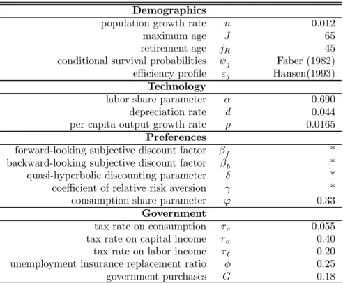
Table 1 summarizes the parameter values of our benchmark model.
2 3For a discussion of the empirical wealth output ratio seeImrohoro˙ ˘glu,˙Imrohoro˘glu, and
Table 1 Calibration Demographics
population growth rate n 0.012
maximum age J 65
retirement age jR 45
conditional survival probabilities ψj Faber (1982) efficiency profile εj Hansen(1993)
Technology
labor share parameter α 0.690 depreciation rate d 0.044 per capita output growth rate ρ 0.0165
Preferences
forward-looking subjective discount factor βf * backward-looking subjective discount factor βb * quasi-hyperbolic discounting parameter δ * coefficient of relative risk aversion γ * consumption share parameter ϕ 0.33
Government
tax rate on consumption τc 0.055 tax rate on capital income τa 0.40 tax rate on labor income τ` 0.20 unemployment insurance replacement ratio φ 0.25 government purchases G 0.18
* Parameter takes on various values as described in Sections 3.2, 4.1, and 4.2
3.5
Solution Method
In most of our simulations, the discrete setD={d1,d2,....,dm}for asset values is chosen so thatd1= 0andm= 4097.The upper bounddmis set so that it is never binding, typically a value of 20 times the annual income of an employed agent.24 We rely on linear interpolation of the value functions so that the choice
variables that enter the utility function are essentially continuous variables, yielding nearly-continuous policy functions.
To compute the measures of agent types, we do not use the forward recursion described in the definition of the recursive stationary equilibrium. Although the forward recursion leads to the same outcome and has the benefit of expositional clarity, the alternative of simulating histories of a large number of individuals has computational advantages. In particular, we followImrohoro˙ glu,˘ Imrohoro˙ ˘glu, and Joines (1998) to calculate the summary statistics of the model economies
2 4Note that with our choice ofm= 4097,the state space has4097
×2points for individuals who are young and4097×2×2points for individuals who are eligible to collect social security benefits. The discrete-state numerical method used in this paper to obtain the policy functions is quite standard. SeeImrohoro˙ ˘glu,Imrohoro˙ ˘glu, and Joines (1995),Imrohoro˙ ˘glu (1998) and the ‘Practical Dynamic Programming’ chapter in Ljungqvist and Sargent (1998).
from these simulations. We start with a newly born agent and randomly draw the employment state and the survival outcome. Given these realizations, we use the optimal policy functions to generate next period’s endogenous state vari-ables.25 We recursively follow this procedure until we receive a death realization,
which occurs no later than age 85. We replicate this procedure for a large num-ber of individuals and compute the summary statistics as averages across the replications. We replicated 100,000 agent histories to match the resulting cohort shares to those calibrated for the U.S. economy.
Our computations start with a guess for the aggregate capital stock, labor input, government transfers and social security benefits, solve the individuals’ dynamic program to obtain the optimal policy functions, simulate a large num-ber of agent histories, compute the average quantities and check whether they are close to the initial guesses. If so, we have a stationary recursive equilibrium; if not, we iterate on this procedure until convergence.
4
Results
We start this section by examining some of the properties of an economy in which all individuals exhibit time-consistent preferences and behavior (βb =βf andδ= 1). This economy is calibrated to yield a capital-output ratio of 2.52 at a social security tax rate of 10%. Table 2 shows the properties of the steady state of this economy at various social security tax rates. With a 10% tax rate, the steady-state consumption-output ratio is 0.635 and the investment-output ratio is 0.183. Because this is a closed economy, the investment-investment-output ratio is also the saving rate. As the social security tax rate is lowered toward zero, we observe a monotonic increase in the capital stock, investment, and consumption. Complete elimination of the pay-as-you-go social security system raises the saving rate to 0.216 and generates 32% more capital, 12% higher output, and 10% more consumption than an economy with a 10% social security tax rate. Table 2 Time-Consistent Preferences τs(%) w r Y C I K L CV (%) 0 2.565 0.060 1.120 0.698 0.242 3.331 0.301 0.00 2 2.522 0.064 1.092 0.684 0.227 3.127 0.298 1.06 4 2.487 0.068 1.068 0.672 0.215 2.962 0.296 2.19 6 2.455 0.071 1.046 0.661 0.205 2.817 0.294 3.39 8 2.419 0.075 1.022 0.648 0.194 2.665 0.291 4.84 10 2.384 0.079 1.000 0.635 0.183 2.522 0.289 6.91 γ= 2.0,βf = 1.00588,δ= 1.0, B = 1.765
2 5We rely on linear interpolation at this stage also to ensure continuity of both the state
The last column of Table 2 examines the welfare at birth of an individual born into the steady state corresponding to each social security tax rate. The relevant welfare criterion is expected lifetime utility as viewed from age 21, the first period of economic life in our model. This criterion, denoted W21,
is described in Section 2.2 and is based on equation (2). According to this criterion, welfare is maximized at a zero tax rate. We can measure the welfare cost of being born into an economy with social security as the consumption supplement (compensating variation) needed to equate the welfare of a newborn individual in that economy to the welfare of an individual born into an economy with no social security. The compensating variation is computed as a fixed percentage increase in consumption at each age. The last column of Table 2 shows these compensating variations, denotedCV. The welfare cost increases faster than linearly in the tax rate so that at a tax rate of 10%, individuals would require an increase in annual consumption of 6.91% to compensate them for living in a world with unfunded social security.
If there were no possibility of dying before the maximum possible ageJ, then the compensating variation for agents with time-consistent preferences would be the same when viewed from any age. The age-specific welfare criteriaWj∗
defined in Section 2.2, however, are contingent on survival to age j∗. These
criteria sum the utility derived from realized consumption and leisure up through agej∗ and the expected utility of future consumption and leisure, where the
expectation discounts for mortality risk. A pay-as-you-go social security system taxes all workers but pays benefits only to those who survive to retirement, effectively raising the rate of return to survivors. Because of this actuarial reward for survival, it is possible that individuals who reach sufficiently advanced ages might prefer social security even if a newborn individual does not. This turns out not to be the case for the economy described here, asWj∗is maximized
at a social security tax rate of zero for allj∗. Table 3 displays the compensating variation required to make individuals of selected ages indifferent between living in an economy with a social security tax rate of 10% and an economy with no social security. Although individuals of all ages prefer a world without social security, the intensity of their aversion declines with age, reflecting the reward to survival. The fact that even the elderly do not favor unfunded social security is due primarily to the effects of such a system in lowering the aggregate capital stock and lifetime earnings and consumption.
Table 3
Welfare Costs of 10% Social Security Tax Rate
Age CV (%)
21 6.91
41 6.46
61 5.47
4.1
Time-Inconsistent Preferences and Behavior
We now consider a world populated by quasi-hyperbolic discounters (βb =βf
andδ<1) who exhibit a form of time inconsistency in preferences that leads to time inconsistency in behavior. Preferences of this sort are characterized by a current one-period discount rate that is higher than future one-period discount rates. This high short-term impatience leads quasi-hyperbolic discounters to postpone saving, and continual deferral may lead these individuals to enter retirement with substantially lower assets than exponential discounters.
4.1.1 The Effect of Quasi-Hyperbolic Discounting on Saving
If social security is to constitute a welfare-improving policy intervention in an economy with this sort of time inconsistency but not in a world of time-consistent preferences, one would expect tofind an economically significant dif-ference in saving behavior between quasi-hyperbolic discounters and exponential discounters. To see whether this is the case, we run a “counterfactual” experi-ment on the exponential economy summarized in Table 2. Specifically, we vary the quasi-hyperbolic discounting parameterδwhile setting all other parameters to the values used in the exponential economy. The social security tax rate is set to 10%. This experiment is counterfactual in that these economies fail to replicate the empirical capital-output ratio of 2.52 whenδ<1.
If δ < 1, the optimal policy functions derived at age j∗ for ages j0 > j∗
will no longer be optimal when an individual arrives agej0. As a consequence
the age-j0 individual will in general deviate from the policy rules derived at any
earlier age. We assume that individuals are aware of this feature of their own behavior and that they choose current consumption, saving, and work effort optimally, taking into account the behavior of their future selves.
Table 4 summarizes the results of varying δ. The levels of output, con-sumption, and capital are normalized to 100.0 in the exponential economy. The results indicate that quasi-hyperbolic discounting does indeed have a significant effect on saving. Whenδ= 0.90, the steady-state capital stock is about 12.5% below its value in the exponential economy, and a δ of 0.85 causes the capi-tal stock to fall almost 20% below the level in the exponential economy. The magnitude of these effects does not depend in any important way on the social security tax rate. For example, in an economy without social security, a value ofδ= 0.90results in a steady-state capital stock 13% below that obtained with
δ= 1.0.
Table 4
Effects of Quasi-Hyperbolic Discounting
δ Y C K K/Y w r
1.00 100.0 100.0 100.0 2.52 2.38 0.079 0.90 94.8 95.4 87.4 2.33 2.30 0.089 0.85 91.9 93.0 81.5 2.24 2.26 0.095
30 40 50 60 70 80 0 1 2 3 4 5 6 7 8 9 10 age as se t hol di ng s δ=1.0 δ=0.9 δ=0.85
Figure 1: Age-Asset Holding Profiles for Different Values ofδ
Figure 1 displays the age-asset profiles for these three economies. The highest profile corresponds toδ= 1.0and the lowest toδ= 0.85.
4.1.2 Social Security in a World of Quasi-Hyperbolic Discounting
Having established the effect of quasi-hyperbolic discounting on saving, we now ask how much social security can improve welfare in such a world. As with the exponential economy described in Table 2, we require that economies with quasi-hyperbolic discounters and a 10% social security tax rate generate a capital-output ratio that matches the historical U.S. average. We do this by appropriately choosing the standard discount factorβf for each value of δ so that each (βf,δ) pair results in a capital-output ratio of 2.52. We then examine the effects of varying the social security tax rate.
Before reporting the results of our social security experiments, however, we first establish a benchmark against which to compare the welfare effects of dif-ferent tax rates. As our benchmark we consider a world in which individuals have a technology that allows them to commit at age 20 to a state-contingent path of lifetime consumption and work effort. From age 21 until death, these individuals follow decision rules that are the same as those implied by δ= 1, and they effectively overcome the short-term impatience implied byδ<1.
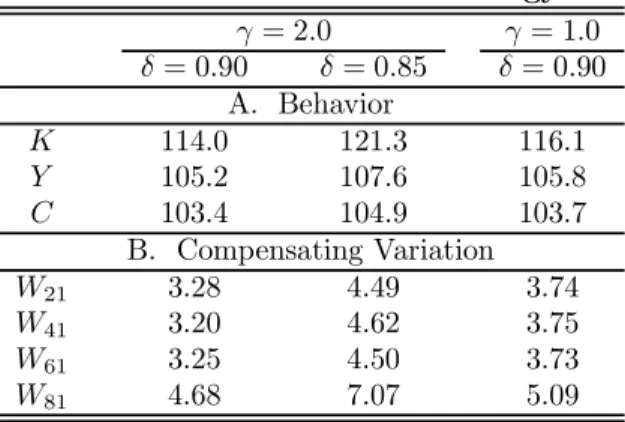
Table 5 summarizes the consequences of a perfect commitment technology for three configurations of preference parameters that we consider in more detail below. The tablefirst reports the levels of capital, output, and consumption, each scaled relative to a value of 100.0 in the no-commitment case without social security. It then gives the value of the commitment technology, expressed as afixed percentage increase in consumption at each age in the no-commitment case that makes individuals as well offas having the commitment device. These compensating variations are computed using preferences as viewed from four dif-ferent ages. The commitment technology results in higher steady-state levels of capital, output, and consumption, and the increase in consumption is con-centrated during retirement years.
Table 5
Perfect Commitment Technology
γ= 2.0 γ= 1.0 δ= 0.90 δ= 0.85 δ= 0.90 A. Behavior K 114.0 121.3 116.1 Y 105.2 107.6 105.8 C 103.4 104.9 103.7 B. Compensating Variation W21 3.28 4.49 3.74 W41 3.20 4.62 3.75 W61 3.25 4.50 3.73 W81 4.68 7.07 5.09
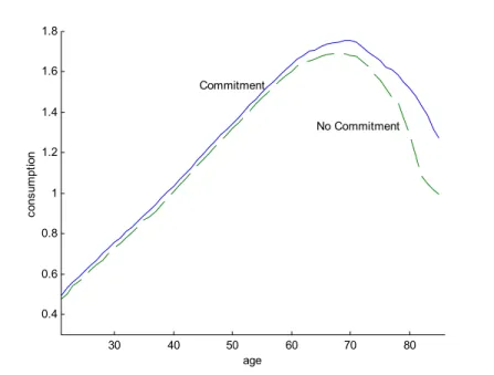
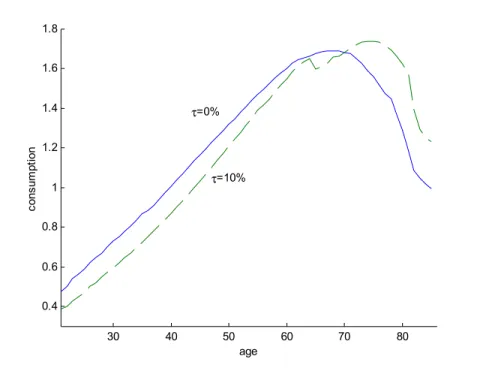
Figure 2 shows the age-consumption profiles for the economy with γ= 2.0 andδ= 0.90in the absence of social security, both with and without the com-mitment device. Both behavior and welfare seem more sensitive to the quasi-hyperbolic discounting parameter than to the inverse elasticity of intertemporal substitution. These results indicate that the steady-state welfare costs to quasi-hyperbolic discounters of their time-inconsistent behavior are substantial.26
We now examine the effectiveness of unfunded social security as a substitute for a perfect commitment technology in maintaing old-age consumption. Table 6 summarizes the economic effects of varying the social security tax rate in economies in which the preference parameters βf, γ, and δ take on different
2 6Laibson (1997, p. 467) reports compensating variations that are much smaller than those
in Table 5. There appear to be two reasons for the difference. First, Laibson’s welfare analysis is for a partial commitment technology that takes the form of an illiquid asset. Second, his analysis is for an infinitely-lived representative agent and includes the change in consumption during the transition from one steady state to another, whereas our comparison is only of the two steady states. Barro (1999, p. 1139) examines the value of perfect commitment. Because he takes into account the transition between steady states, he reports a smaller welfare effect for a given change in steady-state capital than we do. Assuming log utility, hefinds that the value of commitment is small unless the degree of short-term impatience is high.
30 40 50 60 70 80 0.4 0.6 0.8 1 1.2 1.4 1.6 1.8 age co ns um pt io n Commitment No Commitment
Figure 2: Age-Consumption Profiles with and without Commitment
values. The last two parameters are specified a priori, andβf is then chosen to yield a capital-output ratio of 2.52. Our central value forγ, the inverse elasticity of intertemporal substitution, is 2.0. Given γ = 2.0, the quasi-hyperbolic discounting parameterδtakes on values of 1.00 (the exponential case from Table 1), 0.90, and 0.85. In addition, we consider values of γ of 1.0 and 3.0, each paired with aδ of 0.90. The table is normalized so that capital, output, and consumption are all 100.0 when the social security tax rate is 10%, reflecting the fact that allfive economies have been calibrated to yield the same values of these three aggregates.
Social security reduces the steady-state values of capital, output, and con-sumption in each of the economies considered. The results forγ= 2.0indicate that the capital stock would be about 1/3 larger in the absence of social secu-rity. The magnitude of this effect is similar across the three values ofδ, although it is somewhat more pronounced with quasi-hyperbolic discounting. A lower elasticity of intertemporal substitution (γ= 3.0) implies a larger effect of social security on steady-state capital, while γ = 1.0implies a smaller effect. The smaller the elasticity of substitution, the greater the reduction in the saving of workers when the government attempts to reallocate consumption toward retirement years through the payroll tax.
Table 6
Effects of Social Security with Quasi-Hyperbolic Discounting
γ= 2.0 γ= 3.0 γ= 1.0 τs(%) δ= 1.00 δ= 0.90 δ= 0.85 δ= 0.90 δ= 0.90 A. Capital 0 132.0 134.0 136.4 145.7 123.1 2 123.9 125.0 126.8 133.3 119.0 4 117.4 117.7 118.7 123.2 114.6 6 111.7 111.6 111.9 114.6 109.3 8 105.6 105.6 105.5 107.1 104.3 10 100.0 100.0 100.0 100.0 100.0 B. Output 0 112.2 112.9 114.0 116.4 109.5 2 109.4 109.8 110.6 112.5 107.8 4 107.0 107.2 107.6 109.9 106.0 6 104.8 104.8 104.9 105.8 103.8 8 102.4 102.4 102.4 102.8 101.8 10 100.0 100.0 100.0 100.0 100.0 C. Consumption 0 109.9 110.5 111.3 112.6 108.4 2 107.8 108.2 108.9 110.0 106.7 4 105.9 106.2 106.5 107.3 105.3 6 104.1 104.2 104.4 104.9 103.4 8 102.1 102.1 102.1 102.4 101.5 10 100.0 100.0 100.0 100.0 100.0
D. Other Parameter Values
βf 1.0058 1.0117 1.0146 1.0261 0.9980
B 1.7652 1.7740 1.7880 1.7766 1.7625
We can now use these economies to examine the welfare consequences of social security. Although the effect of social security on aggregate consumpton does not seem very sensitive to the value of the quasi-hyperbolic discounting parameter, there are two reasons why the welfare effects might still depend on
δ. First, social security affects not only aggregate consumption but also its allocation over the life cycle, and these intertemporal reallocations might differ across the three values of δ considered. Second, individuals with different δ’s have different preferences, so they value a given lifetime consumpton sequence differently. In addition, the welfare effects might depend onγ. A sharp decline in old-age consumption due to quasi-hyperbolic discounting might have higher welfare costs, and social security might lead to correspondingly larger welfare gains (at least as viewed from old age), the lower the elasticity of intertemporal substitution. But as we have seen, a low elasticity of substitution also raises the costs of social security, which take the form of lower steady-state capital and lifetime consumption.
As noted in Section 2.2, with time-inconsistent preferences we can view a single individual as a collection of J individuals, each of a different age and each with a different set of preferences. Since theseJ individuals need not agree on their ranking of different consumption and labor sequences, we use equation (2) to compute welfare measures Wj∗ for each agej∗ = 1,2, ...J. For social
security tax rates between 2% and 10%, we determine thefirst agebjat whichWbj is greater with social security than without. (It turns out in our experiments that if social security raises welfare as viewed from agebj, it also raises welfare as viewed from any agej >bj.) We also calculate the fraction of the population falling into ages j≥bj.
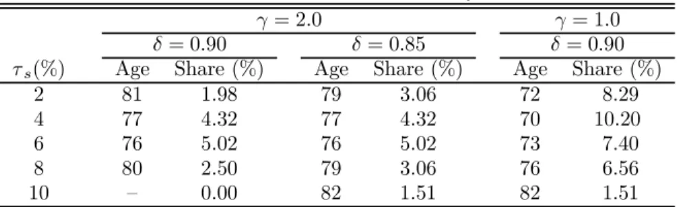
Table 7 reports these welfare calculations for three of the five economies summarized in Table 6. We omit the exponential economy, where even a 2% social security tax rate lowers welfare as viewed from all ages, and the economy withγ= 3.0, where a social security tax rate as high as 10% lowers welfare as viewed from any age.27 In the remaining economies, wefind that social security raises the welfare of quasi-hyperbolic discounters as viewed from sufficiently advanced ages. Withγ= 2.0, the fraction of the population falling into these cohorts never exceeds about 5%, however. Withγ= 1.0, a 4% social security tax rate increases welfare as viewed from ages 70 and greater, corresponding to more than 10% of the population. The aggregate welfare measureW, which weights each of the age-specific indicatorsWj∗by the unconditional probability
of surviving to agej∗, is always higher without social security than with any
of the tax rates considered here. Overall, these results indicate that unfunded social security is not particularly effective in correcting for the undersaving resulting from quasi-hyperbolic preferences, at least for the degrees of myopia considered here.
Table 7
Who Prefers Social Security?
γ= 2.0 γ= 1.0
δ= 0.90 δ= 0.85 δ= 0.90
τs(%) Age Share (%) Age Share (%) Age Share (%)
2 81 1.98 79 3.06 72 8.29
4 77 4.32 77 4.32 70 10.20
6 76 5.02 76 5.02 73 7.40
8 80 2.50 79 3.06 76 6.56
10 — 0.00 82 1.51 82 1.51
In light of the apparently widely held view that social security may raise the welfare of short-sighted individuals who fail to save adequately for their re-tirement, the question arises as to why our model implies such meager welfare
2 7Withγ = 3.0, welfare as viewed from age 85 is maximized with a tax rate of 6%, but
welfare as viewed from any other age is higher with no social security than with any of the tax rates we have examined.