Menu Theorems for Bilateral Contracting

Menu Theorems for Bilateral Contracting

Seungjin Han

McMaster University

October 28, 2003

Abstract

This paper studies the bilateral contracting environment where multiple principals negotiate contracts with multiple agents independently. It is shown that equilibrium allocations associated with (pure strategy) perfect Bayesian equilibria relative to any ad hoc set of negotiation schemes can be supported by pure strategy perfect Bayesian equilibria relative to the set of menus. It is also shown that equilibrium allocations associated with all perfect Bayesian equilibria relative to any ad hoc set of negotiation schemes can be supported by correlated equilibria relative to the set of menus, where the set of states is simply the set of feasible probability distributions over payoff-relevant variables. Moreover, equilibrium allocations associated with all equilibria relative to the set of menus persist even if principals use more complex negotiation schemes.

JEL classification numbers: D82, C79

∗_{Department of Economics, Kenneth Talyor Hall, Room 426, McMaster University 1280 Main Street} West, Hamilton, Ontario, Canada, L8S 4M4. Email:[email protected]. This is a revised version of the first chapter in my PhD dissertation at the University of Toronto. I am deeply indebted to Michael Peters for his insightful guidance and advice. I wish to thank Ettore Damiano, Jeffrey Ely, Martin Osborne, Alessandro Pavan, Carolyn Pitchik, Ilya Segal and seminar participants at the University of Toronto and the 2002 Canadian Economic Theory Conference for numerous helpful comments and discussions. Financial support from Social Sciences and Humanities Research Council of Canada is thankfully acknowledged. All errors are mine alone.

Keywords: mechanism design, bilateral contracting, multiple principals, multiple agents

1

Introduction

Efficiency in markets relies fundamentally on competition. Competing sellers drive down prices and raise quantities, competing auctioneers drive down reserve prices, making it more likely that efficient trades will be consummated. It is natural to expect that these beneficial effects of competition should be independent of the way that sellers compete. So, if many principals compete in incentive contracts, for example, their competition should still ensure that outcomes are close to being efficient.

There are many examples in the literature suggesting that this need not be the case. Klemperer (2002), for example, describes implicit collusion that occurred in British electric-ity auctions with many competitors that results from the fact that prices were determined in a uniform price auction. Klemperer and Meyer (1989) describe the large number of ineffi-cient equilibria that can occur when sellers compete in supply functions. Even though there are equilibria where multiple lobbyists compete away all their rents (Dixit, Grossman and Helpman 1997), there are also many inefficient equilibria in the simplest common agency problem. The bad equilibria in these problems arise in simple static competitive environ-ments so the implicit collusion that occurs has nothing to do with repeated game effects. It does seem to be related to the nature of the competition between sellers. For example, many of the inefficient equilibria described by Klemperer and Meyer (1989) disappear if sellers are simple Cournot competitors.

The complication that arises in environments where sellers compete in more complex ways has been described in the terminology of mechanism design by McAfee (1993). When principals communicate with agents in a competitive environment, the agents have infor-mation about what is happening in the market that principals do not have when they design and offer their incentive contracts. If principals ask their agents about this market information, in other words principals use mechanisms, they may be able to learn when

one of the other principals has deviated from some implicit agreement. This lets them pun-ish deviations and enforce collusive outcomes. In other words, if principals use incentive contracts that are sophisticated enough, they can neutralize the effects of competition.

To overcome the difficulties associated with this, it is important to understand exactly how principals support these collusive outcomes. The recent literature on common agency has provided an important insight into how this is done. Principals offer the single agent menus of alternative incentive contracts. If the agent’s preference ordering over the alterna-tives in these menus depends on what other principals have done, then that is often enough for principals to create the punishments that support collusive outcomes. Theorems in, for example, Martimort and Stole (2002) or Peters (2001) show that all collusive outcomes that principals can support can be understood in exactly this way. Furthermore, from Peters (2001), principals who offer menus of incentive contracts cannot do any better by using more complex mechanisms.

The idea that principals offer an agent menus of alternative incentive contracts from which the agent chooses cannot be extended in any obvious way beyond the common agency framework. When there are multiple agents, mechanisms will typically choose incentive contracts based on the messages of many different agents. There is no way to assign the choice to a single agent, as is the case with simple menus.

The only approach available in the case of multiple agents is the one proposed by Epstein and Peters (1999). They describe a language that agents can use to describe their market information to principals. With this language in place, competition between principals can then be modelled as competition in direct mechanisms. The language that is required to describe type is complex because of the infinite regress involved in characterizing mechanisms.1 So it is of interest to try to find environments where simpler mechanisms might suffice to understand collusion between principals.

This paper studies thebilateral contracting environment where principals can assign an incentive contract for each agent conditional on the message that the agent sends but not

1_{In general type spaces are just as complex in the single principal case. The type space is made simple}

on the messages sent by the other agents. Therefore, multiple principals negotiate incentive contracts with multiple agents independently. In this case, it makes sense to think about the principal offering each agent a menu of incentive contracts because an incentive contract assigned to an agent does not depend on the communication between principals and the other agents so the agent can directly choose an incentive contract from a menu.

Prat and Rustichini (2002) first model a multiple agency problem which can be viewed as a simple bilateral contracting game. In their model, multiple principals offer single incentive contracts to multiple agents. An incentive contract in their model specifies mon-etary payments to an agent conditional on efforts taken by the agent. In the Prat and Rustichini’s model, the incentive contract offered to one agent does not depend on whether or not the other agents take the incentive contracts offered to them. So, the game is bilat-eral contracting. Examples of the Prat and Rustichini’s model include lobbying, vertical contracts, and competing first-price auctions among many others.

It is however important that the Prat and Rustichini’s model restricts principals to offer only a single incentive contract to each agent. No significant market information is revealed by agents because there is no communication between agents and principals. Furthermore, Prat and Rustichini do not address the question of whether equilibrium allocations in their simple model persist even if principals are allowed to use complex mechanisms.

The bilateral contracting game considered in this paper allows principals to offer agents any complex mechanisms that they like. If a principal is able to offer mechanisms so-phisticated enough to induce agents to reveal their market information, the principal can punish other principals’ deviations from implicit collusion by changing his contracts. Even in a static game, equilibria relative to complex mechanisms can support many collusive outcomes that are not supported by any equilibria in the Prat and Rustichini’s model.

This paper shows that the competition relative to the set of menus in common agency in Martimort and Stole (2002) and Peters (2001) can provide a way to characterize equilibrium allocations relative to any set of mechanisms in the bilateral contracting environment in the presence of externalities among players. First of all, it is shown that equilibrium allocations associated with pure strategy perfect Bayesian equilibria relative to any set of mechanisms

can be supported by pure strategy perfect Bayesian equilibria relative to the set of menus. Since pure strategy equilibria are of interest in many applications, this result is especially useful.

The menu theorems for common agency show that perfect Bayesian equilibria relative to the set of menus support equilibria allocations associated with all perfect Bayesian equilibria relative to any set of mechanisms. The theorems are not directly extended into the bilateral contracting environment. With externalities between agents, the optimal incentive contracts in menus and the optimal effort for one agent depend on what this agent believes some other agents do. It is therefore natural to expect multiple continuation equilibria to be associated with menus that principals offer. Principals can correlate different continuation equilibrium allocations by changing the name of their menus. If principals are restricted to use menus, only one continuation equilibrium is assigned at menus that principals offer. Therefore such a coordination is not possible if principals are restricted to use menus. This type of problem does not arise in common agency because a single agent is solely able to decide a continuation equilibrium given menus by choosing incentive contracts in menus offered to her. To illustrate this problem, this paper provides an example of an equilibrium relative to a specific set of mechanisms that cannot be supported by equilibria relative to the set of menus.

This paper proposescorrelated equilibria relative to the set of menus to support equilib-rium allocations associated with mixed strategy equilibria relative to any set of mechanisms. In correlated equilibrium, a state is realized from a probability distribution conditional on a collection of menus offered by principals. A state delivers agents a belief about which equilibrium will occur. Given a state, agents choose their incentive contracts in menus. It is important that an equilibrium allocation is fully characterized by a probability distribu-tion over payoff-relevant variables. If the set of states is the set of all feasible probability distributions over payoff-relevant variables, then any equilibrium allocation relative to any set of mechanisms can be associated with a unique state. It is shown that with this set of states, correlated equilibria relative to the set of menus support equilibrium allocations associated with all perfect Bayesian equilibria relative to any set of mechanisms.

One of the concerns about specifying a set of simple mechanisms in a model of compe-tition is that compecompe-tition relative to a set of simple mechanisms might generate equilibria that disappear once principals are allowed to use more complex mechanisms. Predictions based on such equilibria are questionable because at least conceptually principals should be able to use any mechanisms they like. This paper shows that equilibrium allocations relative to the set of menus are robust in the sense that the equilibrium allocations persist even if the set of mechanisms is enlarged. Predictions based on any equilibrium relative to the set of menus are robust.

2

Preliminaries

Throughout this paper, a set is assumed to be a compact set unless specified. When a measurable structure is necessary, the corresponding Borel σ - algebra is used. For a set X, ∆(X) denotes the set of probability distributions on X. For any x ∈ ∆(X), supp x denotes the support of the probability distribution x. For any mapping L from S into Q, L(S) denotes the image of L.

The set of principals is J = {1,· · · , J}. The set of agents is I = {1,· · · , I}. Each principal j takes an action yj _{from a setY}j _=×I

s=1Ysj. A typical action taken by principal

j is given yj = (y₁j, . . . , y_Ij)∈ Yj. In many competition models in nonlinear prices, y_ij is a monetary payment between principal j and agenti. Y =×J

t=1Yt is the set of actions that

all principals can take.

Each agent i takes an effortei from a set Ei. E =×Is=1Es is the set of efforts that all

agents can take. The principals observe (possibly only partially) the efforts of all agents. Each principal j writes an incentive contract aj_i for each agent i from a set Aj_i which specifies yj_i for each agent i that the principal will take conditional on whatever levels of efforts e = (e1,· · ·eI)∈ E that the principal can verify to the agent. Let Aji be the set of

feasible mappings from E into Y_ij. Aj_i = ∆(Aj_i) is the set of random incentive contracts (henceforth just incentive contracts) that principal j can offer to agent i. Aj _=×I

s=1Ajs is

of incentive contracts that all principals can offer to agent i.A typical element (α1

1,· · · , αJI)

in A =×I

s=1As is called a collection of incentive contracts that all principals can offer to

all agents.

Agent i has private information about her preferences. This information is parame-terized by an element, called a valuation, in a measurable space Ωi. All agents and all

principals share a common prior belief that the elements of Ω = ×I

s=1Ωs are jointly

dis-tributed according to some probability distributionF on Ω. Each principal’s payoff is given by vj _{:Y ×E×Ω→ R and each agent’s payoff is given byu:Y ×E×Ω}

i → R.

2.1

Bilateral contracting

A mechanism for principal j is a collection of message spaces, Cj _=×I

s=1Csj, and a mapping

fromCj _intoAj_{. C}j

s for eachs∈ I is the set of messages that agents can send to principal

j. Without loss of generality, C_ij =C for all i∈ I and all j ∈ J.

The bilateral contracting environment restricts feasible mechanisms that principals can offer to agents. Contracting is bilateral if each principal j offers each agent i a bilateral mechanism (simply mechanism hereinafter)

γ_ij :C → Aj_i

that describes incentive contracts for agenticonditional on the messages that agentisends. Let Γj_i be a set of feasible mechanisms that principalj can offer to agent i. Γj =×I

s=1Γjs is

the set of mechanisms that principaljcan offer to all agents. A typical element (γ1

1,· · · , γIJ)

in Γ = ×J

t=1Γt is called a collection of mechanisms that all principals offer to all agents.

A bilateral contracting game begins when each principal simultaneously offer mecha-nisms, one for each agent. After seeing the collection of mechanisms offered by principals, each agent simultaneously sends a message to each principal and chooses her effort.2

Sub-sequently, all payoffs are realized.

2_{As the literature on mechanism design assumes, each principal fully commits himself to inform agents}

of his negotiation schemes. So, each agent knows mechanisms offered to the other agents when she sends messages.

While bilateral contracting between multiple principals and multiple agents is very often observed in practice, there is very little literature on it. Recently, Prat and Rustichini (2002) consider a delegation game under complete information which can fit into bilateral contracting between multiple principals and multiple agents. In the Prat and Rustichini’s model, each principal j offer an incentive contract aj_i : Ei → Yij to each agent i, where a

typical elementy_ij inY_ij is a monetary payment from principalj to agenti. Given contracts, each agent i chooses an effort ei ∈ Ei that determines payoffs. An incentive contract aji

can be interpreted as a degenerate mechanism γ_ij :C → Aj_i that satisfiesγ_ij(cj_i) =aj_i for all cj_i ∈ C. The game in which each principal offers a single incentive contract to each agent is therefore a bilateral contracting game.

Examples in the Prat and Rustichini’s delegation game include lobbying games, vertical contracts, and competing first-price auctions among many others. In lobbying game, an effort ei ∈ Ei chosen by policy maker i (an agent) is a policy. The ith component yij in

an action yj _{is a monetary contribution made by lobbyist j (a principal). Each lobbyist j}

offers each policy maker i a monetary contribution scheme aj_i :Ei →Y j i .

3

In vertical contracts, many upstream firms (for example, IBM and Apple, principals) compete for inputs produced by many downstream firms (for example, D-Ram from Sam-sung and S-Ram from NEC, agents). The ith component y_ij in an action yj is a monetary payment by an upstream firm j (a principal) to a downstream firm i (an agent). Each downstream firmisupplies an input to each upstream firm that is necessary for production. Therefore, a typical effort ei consists of j components: ei = {e1i,· · · , eJi} ∈ Ei = ×Jt=1Eit.

ej_i is an amount of the input supplied by downstream firm i to upstream firm j. Each upstream firm j offers a demand schedule aj_i :E_ij →Y_ij to each downstream firm i.4

In competing first-price auctions, each buyer j (a principal) submits a bid function to each auctioneeri(an agent). A typical action that buyeritakes isyi ={y1j,· · · , y

j

I} ∈Yj =

×I

s=1Ysj, wherey j

i is a monetary payment from buyerjto auctioneeri. Each auctioneerihas

3_{Dixit, Grossman, and Helpman (1997) construct a lobbying game in a common agency framework.} 4_{Many examples of vertical contracts in a single-principal-multi-agent framework can be founded in}

a divisible object. A typical objecteiis therefore expressed by an arrayei ={e1i,· · · , eJi} ∈

Ei = ×Jt=1Eit, where e j

i is the fraction of the object that auctioneer i sells to buyer i. a j i

: E_ij → Y_ij is a bid function submitted by buyer i to auctioneer j. Given bid functions submitted by buyers, each auctioneer allocates his divisible object to maximize the revenue.5

While Prat and Rustichini provide a simple game to analyze bilateral contracting, it is important that in their game, principals are only allowed to offer single incentive contracts to agents. There is no market information that agents reveal to principals since agents decide only whether or not they take incentive contracts offered by principals. It restricts a principal’s ability to change his contracts in response to market changes. If a principal offers mechanisms sophisticated enough to induce agents to reveal their market information about what other principals are doing, the principal is able to punish other principals’ deviations from implicit collusion by changing his contracts. Even in a static game, equilibria relative to complex Γ can support many collusive outcomes that are not supported by equilibria in the Prat and Rustichini’s game.

Prat and Rustichini do not allow a random incentive contract. An incentive contract aj_i in Prat and Rustichini is also restrictive in the sense that monetary payments to agenti depend only on the effort that agent i takes. When an incentive contract makes monetary payments to an agent contingent on all the agents’ efforts (aj_i : E → Y_ij), it creates strategic externalities between agents. This strategic externalities can be used as a device to coordinate agents’ efforts even without direct externalities between agents.

3

Equilibrium in Bilateral contracting Games

This section constructs a bilateral contracting game relative to some arbitrary Γ. The communication behavior and the effort decision for each agent i depend on the realized valuation on her preferences and a collection of mechanisms that all principals offer. A

5_{Bernheim and Whinston (1986) model the single first-price auction for divisible goods under complete}

information. In the Bernheim and Whinston’s model, multiple buyers, interpreted as principals, submit their bid functions to the single auctioneer, interpreted as a common agent.

continuation strategy mifor agenti∈ Iis a measurable mapping from Γ×Ωiinto ∆(CJ×Ei)

that describes the joint probability distribution onCJ_×E

ithat agentiwill use as a function

of agent i’s valuation and a collection of mechanisms offered by principals.

mi : Γ×Ωi →∆(CJ ×Ei)

where CJ _{is the set of messages that agentican send to all principals. With a slight abuse}

of notation, mi(·,·|γ, ωi) is the probability distribution on CJ ×Ei that agenti uses when

γ = (γ1

1,· · · , γIJ) ∈ Γ is the collection of mechanisms that principals offer to agents and

agent i’s valuation is ωi ∈Ωi.6

A profile of continuation strategies m_e = (m_e1,· · · ,meI) is a continuation equilibrium

relative to Γ if for every i ∈ I, every γ ∈Γ, and every ωi ∈ Ωi, the continuation strategy

e

mi maximizes

Z

u(a(e), e, ωi)dγ(c)dme−i(c−i, e−i|γ, ω−i)dF(ω−i|ωi)

whereF(·|ωi) is the probability distribution over the other agents’ valuations conditional on

agent i’s valuation ωi, e = (e1,· · ·eI), a(e) = (a11(e),· · ·aJI(e)), and me−i(c−i, e−i|γ, ω−i) = e

m1(c1, e1|γ, ω1)×· · ·×mei−1(ci−1, ei−1|γ, ωi−1)×mei+1(ci+1, ei+1|γ, ωi+1)×· · ·×meI(cI, eI|γ, ωI).

Fix a continuation equilibriumm_e relative to Γ. One can derive fromm_ei the probability

distribution πi on Ai ×Ei for agent i given any γ ∈ Γ and any ωi ∈ Ωi7. Given the

continuation equilibriumm_e relative to Γ, the probability distributionπonA×Econditional

6_{One natural alternative to construct the agent’s decision process is that agents simultaneously send}

messages to principals and then simultaneously decide efforts without observing messages sent by other agents and contracts assigned to other agents. In this case, a communication strategy hi is a mapping from Γ×Ωi into ∆(CJ). An effort strategyi is a mapping from Γ×Ωi× CJ into ∆(Ei). For any pair of a communication strategy hi and an effort strategy i, there is a corresponding continuation strategy mi such that for every γ∈Γ,and everyωi∈Ωi,

mi(ci, ei|γ, ωi) =i(ei|ci, γ, ωi)×hi(ci|γ, ωi) (1)

whereci= (c1i,· · · , c J i)∈ C

J _{is an array of messages that agentisends to principals. For any continuation} strategy mi, there is also a pair of a communication strategy hi and an effort strategy i satisfying (1). Therefore, two approaches are strategically equivalent.

7_{The fact thatπ}

on any γ ∈Γ and any ω = (ω1,· · · , ωI)∈Ω is

π(α, e|γ, ω) =π1(α1, e1|γ, ω1)× · · · ×πI(αI, eI|γ, ωI)

where α= (α1

1,· · · , αJI)∈ A and αi = (αi1,· · · , αJi)∈ Ai for all i∈ I.

Given any γ ∈Γ and any ωi ∈Ωi, agent i’s equilibrium payoff is

U(m, γ, ω_e i) = (2)

Z

u(a(e), e, ωi)dα(a)dπ(α, e|γ, ω)dF(ω−i|ωi)

Principal j ∈ J chooses a strategy σj _{from ∆(Γ}j_{). σ}j_(γj_{) is the probability that}

principal j offers the array of mechanisms γj = (γ₁j,· · · , γ_Ij)∈ Γj. Suppose that the other principals’ strategies are

σ−j(γ−j) = {σ1(γ1),· · · , σj−1(γj−1), σj+1(γj+1),· · ·, σJ(γJ)}

Principal j’s payoff associated with a strategy σj _is

Vj(σj, σ−j,m) =_e

Z

vj(a(e), e, ω)dα(a)dπ(α, e|γ, ω)dF(ω)dσj(γj)dσ−j(γ−j)

(σ,_e m) is a_e Perfect Bayesian Equilibrium (PBE) relative to Γ such that _eσ= (_eσ1_{,· · · ,}

e

σJ_{) is}

a Nash equilibrium for the normal form game defined by the continuation equilibrium m_e relative to Γ.

4

Menus and Nature of Competition

A menu can be thought of as a simple mechanism with the message space equal to a set of incentive contracts. Among alternatives of incentive contracts, an agent simply picks up some incentive contract that she likes. A menu γj_i is a measurable mapping from Aj_i into

Aj_i satisfying γj_i(αj_i) =    αj_i αj_i ∈Z e αj_i αj_i ∈/ Z

for some closed subset Z ⊂ Aj_i, where γj_i(αj_i) is the incentive contract that principal j assigns when agent i chooses αj_i and α_ej_i is an arbitrary incentive contract in Z. Let Γj_i be the set of all menus that principal j can offer to agent i. Γj =×I

s=1Γ

j

s is the set of menus

that principal j can offer to all the agents. Γ = ×J t=1Γ

t

is the set of collections of menus that all principals can offer to all agents. Let (_bυ,_bq) be a PBE relative to Γ. Theorem 1 shows that equilibrium payoffs for principals and agents associated with pure strategy equilibria relative to any Γ are preserved as equilibrium payoffs by pure strategy equilibria relative to Γ.8

Theorem 1 Let (_eγ, ,m)_e be a pure strategy PBE relative to any Γ. Then, there exists a

pure strategy PBE (_bγ,q)_b relative to Γ such that

1. ∀i∈ I, ∀ωi ∈Ω,

U(m,_{e e}γ, ωi) =U(q,bbγ, ωi)

2. ∀j ∈ J,

Vj(_eγj,_eγ−j,m) =_e Vj(_bγj,_bγ−j,_bq)

Proof. See Appendix 9.1.

It is worthwhile to compare theorem 1 with the menu theorems for common agency. Menu theorems for common agency show that equilibria relative to Γ preserve equilibrium payoffs for principals and agents associated with all equilibria relative to any Γ, but theorem 1 shows that in bilateral contracting, pure strategy equilibria relative to Γ preserve equi-librium payoffs for principals and agents associated with pure strategy equilibria relative to any Γ. The key point of theorem 1 is that we only need to convert some communication

8_{If Γ is smaller than Γ, then it might be possible that some pure strategy equilibria relative to Γ cannot}

be reproduced by any of equilibria relative to Γ. However, it implies that those equilibria are no longer equilibria once principals are allowed to use more complex mechanisms such as menus. Those equilibria are not interesting because at least conceptually principals can use any mechanisms they like. Section 1.5 shows that any equilibria, including mixed strategy equilibria, relative to Γ are weakly robust in the sense that they are still equilibria even if principals are allowed to use more complex mechanisms.

and effort decisions for agents off the equilibrium path in the original game into agents’ decisions off the equilibrium path in the game relative to Γ in a way that any unilateral deviation by a principal in Γ is unprofitable.

Fix a pure strategy PBE (_eγ,m) relative to any Γ. First, a mapping_e G : Γj_i → Γj_i for all i ∈ I and all j ∈ J is constructed as follows. Consider an arbitrary menu γj_i. If γj_i(Aj_i) is the same as the image of the equilibrium mechanism _eγ_ij(C_ij), G(γj_i) = _eγ_ij. Otherwise, G(γj_i) is an arbitrary mechanism γ_ij satisfying γ_ij(C) = γj_i(Aj_i). For all i ∈ I, the equilibrium probability distribution πi(·,·|G(γ11),· · · , G(γJI), ωi) onAi×Ei conditional

on (G(γ1₁),· · · , G(γJ_I), ωi) can be derived from mei.

A continuation equilibrium q_b= (_bq1,· · · ,qbI) relative to Γ is constructed as follows. The

continuation strategy q_bi for agent i satisfies

b qi(·,·|γ11,· · · , γ J I, ωi) =πi(·,·|G(γ11),· · ·, G(γ J I), ωi) (3)

for every collection of menus γ = (γ1

1,· · · , γJI)∈Γ and every valuation ωi ∈Ωi.

Unlike common agency, agent i’s payoff directly depends on incentive contracts and efforts chosen by other agents because of externalities between agents. When the continu-ation strategy for agent i is constructed to satisfy (3), π−i(α−i, e−i|G(γ11),· · ·, G(γJI),·) =

Q

s6=iπs(αs, es|G(γ11),· · ·, G(γJI),·) is the probability distribution over incentive contracts

and efforts chosen by the other agents when the collection of menus is (γ1₁,· · · , γJ_I)∈Γ. In the original game, the equilibrium continuation strategy for agent i maximizes her payoff given π−i(·,·|G(γ11), · · · , G(γJI), ·). Since agent i can directly choose any incentive

contract in the corresponding menu that she could have chosen in any mechanism, any mechanism and its corresponding menu provide the same choice set of incentive contracts. Therefore, it is optimal for agent i to use the communication strategyq_bi that satisfies (3).

When each principal j offers menus (_bγ₁j,· · · ,γ_bIj) ∈ Γj such that for all i ∈ I, the image of _bγ_ij is equal to the image of the equilibrium mechanism _eγ_ij in the original game, the equilibrium probability distribution chosen by each agent i in the game relative to Γ is πi(·,·|eγ

1

1,· · · ,eγ

J

I, ωi) for all ωi ∈ Ωi. The equilibrium probability distribution over

in the original game are preserved when principals offer the menus corresponding to the equilibrium mechanisms.

Suppose that some principal j unilaterally deviates to some menus (γj₁,· · · , γj_I) ∈ Γj in the game relative to Γ. By the construction of the continuation equilibrium relative to Γ, this principal will get the same payoff as the one he gets when he deviates to some mechanisms in the original game that can be converted into (γj₁,· · · , γj_I). Therefore any deviations by each principaljin Γj do not generate higher payoffs than does the equilibrium array of menus. So,equilibrium payoffs associated with pure strategy equilibria relative to any Γ are preserved as equilibrium payoffs by pure strategy equilibria relative to Γ.

5

Robust Equilibria

One of the concerns about specifying a set of simple mechanisms is that competition relative to the set of simple mechanisms might generate equilibria that disappear once principals are allowed to use complex mechanisms. Predictions from such equilibria might be questionable because at least conceptually principals can use any mechanisms.

Theorem 1 shows that as long as our attention is equilibrium payoffs associated with pure strategy equilibria, Γ is enough to reproduce equilibrium payoffs associated with pure strategy equilibria relative to any Γ. This is particularly important because pure strategy equilibria are of interest in many applications. This section asks whether the competition relative to the set of menus generates robust equilibria in bilateral contracting in the sense that all equilibria relative to Γ persist even if the set of mechanisms is enlarged.

Peters (2001) shows that in common agency, there is always a way to assign a continu-ation equilibrium relative to any Γ bigger than Γ such that equilibrium payoffs associated with equilibria relative to Γ are equilibria payoffs relative to any Γ. Therefore, any equilib-rium relative to Γ is weakly robust. Formally, Γ =×i,jΓji is bigger than Γ =×i,jΓ

j

i (Γ<Γ)

if there exists an embedding η : Γ → Γ. It implies that there are more mechanisms in Γ than in Γ. The weak robustness of equilibria relative to Γ in common agency also holds in bilateral contracting.

Theorem 2 Let (_bυ,_bq) be a PBE relative to Γ. For every compact metric Γ_<Γ and every PBE (_bυ,_bq) relative to Γ, there exists a PBE (σ,_e m)_e relative to Γ that preserves equilibrium payoffs associated with a PBE (_bυ,q)_b relative to Γ.

proof. See Appendix 9.2

Consider an equilibrium relative to Γ. A principal knows that there are no other menus that provide higher payoffs for him than do menus in the support of his equilibrium strat-egy. Suppose that Γ is bigger than Γ. A principal will deviate to mechanisms in the new set if it is profitable. Suppose that for example, (γ1

1, γ12,· · · , γJI) is a collection of menus

that principals offer to agents. If principal 1 unilaterally deviates and offers agent 1 γ1 1

in Γ1₁ while the other principals still offer agent 1 menus, (γ₁1, γ1₂,· · · , γJ_I) is the collec-tion of mechanisms. Agent 1 might choose different incentive contracts in the mechanisms (γ1

1, γ21,· · · , γJ1) offered to her and subsequently a different effort. The reason is that γ11

might make some other agents believe that agent 1 would choose different incentive con-tracts and a different effort. So, these agents might change incentive concon-tracts and efforts that they choose. Even if the mechanism γ1

1 offers agent 1 the same menu of alternatives

asγ1₁, it may trigger a new continuation equilibrium in which agent 1 is worse off while the principal is better off. This possibility does not arise in common agency. In bilateral con-tracting, this is an important reason why some principal might like to deviate to complex mechanisms in order to coordinate agents’ behavior in his interest.

Any mechanism γ_ij in Γj_i has the corresponding menu γj_i in Γj_i. The choice sets of incentive contracts that γ_ij andγj_i provide are exactly the same. It follows that each agent’s equilibrium communication and effort decision at any collection of complex mechanisms can be constructed to choose the same incentive contracts and the same effort that she could have chosen at a collection of corresponding menus in the continuation equilibrium relative to Γ. If a principal deviates to mechanisms that can be converted into menus in the support of his equilibrium strategy relative to Γ, his payoff is the same as the equilibrium payoff relative to Γ. If he deviates to mechanisms that can be converted into menus outside of the support of his equilibrium strategy, his payoff is no higher than the equilibrium payoff

relative to Γ.

From theorem 1 and theorem 2, we can conclude that the set of equilibrium payoffs associated with pure strategy equilibria relative to Γ is the same as the set of equilibrium payoffs associated with pure strategy equilibria relative to any Γ _< Γ and that the set of equilibria payoffs associated with all equilibria relative to Γ is a subset of the set of equilibrium payoffs associated with all equilibria relative to any Γ _<Γ.

6

Mixed Strategy Equilibria

Theorem 1 shows that equilibrium payoffs associated with pure strategy equilibria relative to any Γ can be preserved by pure strategy equilibria relative to Γ. It still remains to an-swer the question of whether equilibrium payoffs associated with mixed strategy equilibria relative to any Γ can be preserved by equilibria relative to Γ. This question is directly related to the externalities between agents and the complexity of mechanisms in Γ.

With externalities between agents, optimal incentive contracts and efforts for one agent depend on incentive contracts and efforts that other agents choose. It is therefore natural to expect different continuation equilibria, which generate different payoffs for principals, at different collections of mechanisms in Γ even if these different collections are converted into one collection of menus (γ1₁,· · ·, γJ_I). Principals can correlate these different continuation equilibria by randomizing their mechanisms. If principals are restricted to use menus, only one continuation equilibrium is assigned at the collection of menus (γ1

1,· · · , γJI). Therefore

such a coordination is not possible. This type of problems does not arise in common agency because there is only one agent in the model. Example 3 provides a mixed strategy equilibrium relative to some Γ whose payoffs cannot be preserved by equilibria relative to Γ.

Example 3 There are two principals and two agents with complete information and agents

take no effort. The set of actions is Y1 =Y2 ={(a, a),(a, b),(b, a),(b, b)}, where the first component in each action is for agent 1 and the second component for agent 2. The payoffs for each player are given by

a, a a, b b, a b, b a, a 0,0,10,10 4,2,4,4 0,0,10,10 4,1,2,4 a, b 0,0,10,10 5,6,4,3 0,0,10,10 7,3,4,4 b, a 0,0,10,10 0,0,10,10 0,0,10,10 0,0,10,10 b, b 0,0,10,10 0,0,10,10 0,0,10,10 0,0,10,10 Table 1: Payoffs

Each cell in the first row coincides with an action chosen by principal 2: the first component for agent 1 and the second for agent 2. Each cell in the first column is an action chosen by principal 2: the first component for agent 1 and the second for agent 2. The numbers in the cells give the payoffs for principal 1, principal 2, agent 1, and agent 2 respectively.

Suppose that principals are restricted to offer menus to agents. There are three menus in this example: ma ={a}, mb ={b}, andm={a, b} that each principal can offer to each

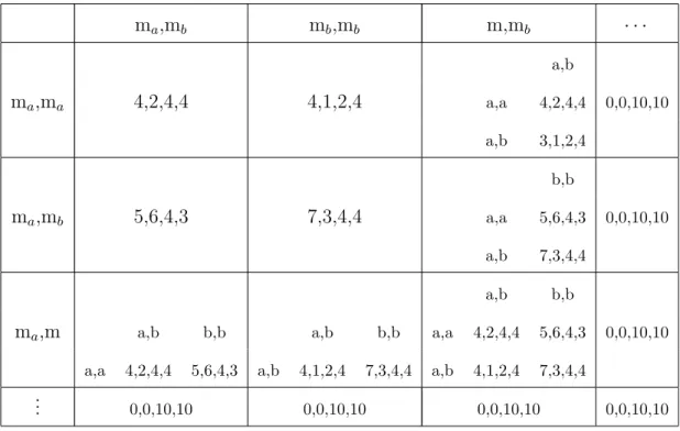
agent. Each principal offers menus, one for each agent. Each agent chooses components from menus offered to her. Table 2 summarizes subgames played by agents given arrays of menus.

Each cell in the first row coincides with a pair of menus offered by principal 2: the first menu to agent 1 and the second to agent 2. Each cell in the first column coincides with a pair of menus offered by principal 1: the first menu to agent 1 and the second to agent 2. Suppose that principal 1 offers (ma, m) and principal 2 offers (m, mb). Agent 1 must

choose the component ain the principal 1’s menuma because there is no other component

that she can choose in ma. But, she can choose either a or b in the menu m offered by

principal 2. Agent 2 can choose either a or b in the menu m offered by principal 1 while b is the only choice in the menu mb offered by principal 2. Agents play the 2×2 normal

form game described in the corresponding cell in table 2. There are only two equilibria in this game. One is that agent 1 chooses a in both principals’ menusma and m respectively

ma,mb mb,mb m,mb · · · a,b ma,ma 4,2,4,4 4,1,2,4 a,a 4,2,4,4 0,0,10,10 a,b 3,1,2,4 b,b ma,mb 5,6,4,3 7,3,4,4 a,a 5,6,4,3 0,0,10,10 a,b 7,3,4,4 a,b b,b

ma,m a,b b,b a,b b,b a,a 4,2,4,4 5,6,4,3 0,0,10,10

a,a 4,2,4,4 5,6,4,3 a,b 4,1,2,4 7,3,4,4 a,b 4,1,2,4 7,3,4,4 ..

. 0,0,10,10 0,0,10,10 0,0,10,10 0,0,10,10

Table 2: Subgames played by agents

other is that agent 1 chooses ain the principal 1’s menumaand bin the principal 2’s menu

m and agent 2 choosesb in both principals’ menus m and mb respectively.

Suppose that principal 1 offers (ma, m) and principal 2 offers (mb, mb). Agent 1 must

choose ain the principal 1’s menu ma andb in the principal 2’s menumb. Agent 2 chooses

either a or b in the principal 1’s menu m but only b in the principal 2’s menu mb. In this

case, agent 2 is indifferent between aand b from principal 1.So, it is optimal for agent 2 to choose a with probabilitypand b with probability 1−pfrom principal 1 for any p∈[0,1]. Consider the case where principal 1 offers (ma, mb) and principal 2 offers (m, mb). Agent

2 chooses b in both principals’ menus mb and mb respectively. Agent 1 can choose eithera

or b in the principal 2’s menu m but onlya in the principal 1’s menu ma. Since agent 1 is

indifferent between two components in the principal 2’s menu m in this case, it is optimal for agent 1 to choose a with probability r and b with probability 1−r in the principal 2’s menu m, where r∈[0,1].

Given strategies p and r, principals play a normal form game given by table 3, where p∈[0,1], r∈[0,1], z ∈ {0,1}.

ma, mb mb, mb m, mb · · · ma, ma 4,2 4,1 4,2 0,0 ma, mb 5,6 7,3 7−2r,3 + 3r 0,0 ma, m 4,2 7−3p,3−2p 7−3z,3−z 0,0 .. . 0,0 0,0 0,0 0,0

Table 3: A continuation equilibrium relative to the set of menus

Consider a bilateral contracting game relative to some Γ = Γ1

1×Γ12×Γ21×Γ22. Suppose

that Γj_i = {γa, γb, γ, γ 0

} for all j ∈ {1,2} and all i ∈ {1,2}. For simplicity C = M. In particular, the image of mechanisms satisfies γa(M) = {a}, γb(M) = {b}, and γ(M) =

γ0(M) = {a, b}. Note that essentially γ and γ0 provide the same choice set of alternative components although each mechanism can require different messages to assign the same component.

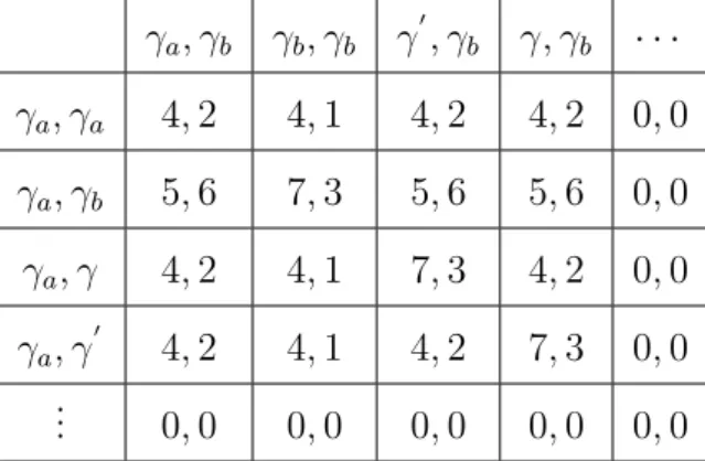
One possible normal form game defined by a continuation equilibrium relative to Γ is

γa, γb γb, γb γ 0 , γb γ, γb · · · γa, γa 4,2 4,1 4,2 4,2 0,0 γa, γb 5,6 7,3 5,6 5,6 0,0 γa, γ 4,2 4,1 7,3 4,2 0,0 γa, γ 0 4,2 4,1 4,2 7,3 0,0 .. . 0,0 0,0 0,0 0,0 0,0

Table 4: A continuation equilibrium relative to Γ

A mixed strategy equilibrium in the normal form game is that principal 1 offers (γa, γ) or

(γa, γ 0

) with equal probability and principal 2 offers (γ, γb) or (γ 0

, γb) with equal probability.

In this equilibrium, principal 1 gets 5.5 and principal 2 gets 2.5. Both agents always get 4. These equilibrium payoffs are never supported by any equilibria relative to Γ. Two pairs of mechanisms (γ0, γb) and (γ, γb) offered by principal 2 are converted into the pair of menus

(m, mb). Two pairs of mechanisms (γa, γ) and (γa, γ 0

into the pair of menus (ma, m). If we restrict principals to use menus, then either only

(7,3) or only (4,2) is assigned as payoffs for principals when principal 1 offers (ma, m) and

principal 2 offers (m, mb). Principals cannot make their actions correlated in a way that

they do in the equilibrium relative to Γ. In general, menus restrict a principal’s ability to correlate his actions across agents in his interest.

7

Correlated Equilibria relative to Menus

Example 3 highlights the reason why equilibrium payoffs associated with some mixed strat-egy equilibria relative to some Γ cannot be preserved by equilibria relative to Γ. Consider different collections of mechanisms in Γ that can be converted into one collection of menus in Γ. Since there are externalities between agents, it is natural to expect that agents act differently at different collections of mechanisms and induce different continuation equi-libria, which generate different payoffs for principals. Essentially, names of mechanisms coordinate agents’ choices over incentive contracts. In other words, they deliver agents a belief about which equilibrium will occur and agents’ optimal behavior confirms the belief in equilibrium.

This type of equilibria is closely related to correlated equilibria. This section considers correlated equilibria relative to Γ. There is a mapping ζ from Γ into the set of probability distributions over the set of states S.

ζ : Γ→∆(S)

A mappingζis called a random state mapping. With a slight abuse of notation,ζ(·|γ1₁,· · · , γJ_I) is a probability distribution on S when (γ1

1,· · · , γJI) is a collection of menus offered by all

the principals. For each i ∈ I, an information partition mapping Pi is a mapping from

Γ×Ωi into Ξ, where Ξ is the set of all feasible partitions of S. P = (P1,· · ·,PI) is called

a profile of information partition mappings.

First, principals simultaneously offer menus to agents. A collection of menus determines a probability distribution on S. A state is realized from the probability distribution. After

seeing a collection of menus and a state, each agent simultaneously chooses an effort and incentive contracts from menus that principals offer to her.

A continuation strategy gi for agent i ∈ I is a measurable mapping from Γ×S×Ωi

into ∆(Ai×Ei) that describes the joint probability distribution over Ai×Ei that agent i

will use as a function of a collection of menus, a state, and agent i’s valuation.

(ζ, S,b Pb,_bg) is a continuation equilibrium relative to Γ if (a) _bg_i(·|γ, s, ω_i) = _bg_i(·|γ, s

0 , ωi)

whenever s ∈ Pi and s 0

∈ Pi for some Pi ∈ Pi(γ, ωi) for each i ∈ I given any γ =

(γ1

1,· · · , γJI) ∈ Γ and any ωi ∈ Ωi and (b) for every i ∈ I, every s ∈ S, every γ =

(γ1₁,· · · , γJ_I)∈Γ,and every ωi ∈Ωi,the communication strategy bgi maximizes

U(g, γ, s, ω_b i) =

Z

u(a(e), e, ωi)dα(a)dbg−i(α−i, e−i|γ, s, ω−i)dF(ω−i|ωi)

where_bg−i(α−i, e−i|γ, s, ω−i) = bg1(α1, e1|γ, s, ω1)×· · ·×bgi−1(αi−1, ei−1|γ, s, ωi−1)×bgi+1(αi+1,

ei+1|γ, s, ωi+1)× · · · ×gbI(αI, eI|γ, s, ωI).

Principalj ∈ J chooses a strategy νj _{from ∆(Γ}j_{). ν}j_(γj_{) is the probability that}

princi-pal j offers the array of menus γj = (γj₁,· · · , γj_I)∈ Γj. Suppose that the strategies chosen by the other principals are ν−j_(γ−j_{) = (ν}1_(γ1_{),· · · , ν}j−1_(γj−1_{), ν}j+1_(γj+1_{),· · · , ν}J_(γJ_)).

Principal j’s payoff associated with a strategy νj _is

Vj(νj, ν−j,_bg) =

Z

vj(a(e), e, ω)dα(a)_bg(α, e|γ, s, ω)dζ(s|γ)dνj(γj)dν−j(γ−j)dF(ω)

where _bg(α, e|γ, s, ω) = _bg(α1, e1|γ, s, ω1) × · · · × g(αb I, eI|γ, s, ωI) with α = (α1,· · · , αI),

e = (e1,· · ·, eI), and ω = (ω1,· · · , ωI). (ζ, S,b Pb,_bg,_bν) is a Correlated Equilibrium (CE)

relative to Γ such that _bν = (_bν1_{,· · ·,}

b

νJ_{) is a Nash equilibrium for the normal form game}

defined by the continuation equilibrium (ζ, S,b Pb,g_b) relative to Γ.

The key question is how bigS should be in order to preserve equilibrium payoffs asso-ciated with all equilibria relative to any Γ as equilibrium payoffs assoasso-ciated with correlated equilibria relative to Γ. Theorem 4 shows that if S = ∆(Y ×E×Ω), equilibrium payoffs associated with all equilibria relative to any Γ can be preserved by correlated equilibria relative to Γ.

Theorem 4 Let (σ,_e m)_e be a PBE relative to any Γ. Suppose that S = ∆(Y ×E ×Ω). Then, there exists a CE (ζ, S,b Pb,

b

g,ν)_b relative to Γ satisfying

1. ∀i ∈ I, ∀γ ∈ ×J

t=1supp σe

t_,∀ω

i ∈ Ωi, there exist γ ∈ ×Jt=1supp νb

t _{and s ∈ supp} b ζ(γ) such that U(m,_{e e}γ, ωi) = U(bg, γ, s, ωi) 2. ∀j ∈ J Vj(_eσj,_eσ−j,m) =_e Vj(ν_bj,_bν−j,_bg)

Proof. See Appendix 9.3.

Theorem 4 shows that for any equilibrium relative to any Γ, there exists a pair of a random state mapping and a profile of equilibrium strategies such that equilibrium payoffs associated with any equilibria relative to any Γ can be preserved as equilibrium payoffs associated with correlated equilibria relative to Γ. It implies that there is no additional equilibrium allocation that one can learn by modelling competition between principals relative to complex Γ instead of modelling it relative to Γ.

The key point of theorem 4 is how to chooseS and to constructζ.b For any collection of

menus γ ∈Γ, there exist many collections of mechanisms in Γ that can be converted into γ. For all γ = (γ1

1,· · · , γJI) ∈ Γ, let ξ(γ) = ×k∈I,t∈Jξ_st(γt_s) be the set of such collections

of mechanisms, where ξ_st(γt_s) is the set of mechanisms in Γt_s that can be converted intoγt_s. Different collections of mechanisms in ξ(γ) may induce different equilibrium allocations be-cause of externalities between agents. It is however important that equilibrium allocations, which decide equilibrium payoffs, are fully characterized by a probability distribution on Y ×E×Ω at any collection of mechanisms. Therefore,S can be as small as ∆(Y ×E×Ω) in the sense that there is a unique probability distribution onY ×E×Ω corresponding to any equilibrium allocation at any collection of mechanisms in ξ(γ). On the equilibrium path, a probability distribution on ∆(Y ×E×Ω) conditional onξ(γ) can be derived from equilib-rium strategies_eσused by principals in the original game. This isζ(b·|γ) =

e

σ(·|ξ(γ))∈∆(S). The strategies _bν for principals are induced fromσ_e used by principals in the original game.

An equilibrium allocation that occurs with a positive probability in the original game is realized as the form of the corresponding state with a positive probability in the new game. After seeing a collection of menus and a state, each agent i has the same belief about which equilibrium will occur. In the new game, agents use probability distributions over incentive contracts and efforts induced by their equilibrium continuation strategies in the original game that generate the realized state, that is a probability distribution over Y ×E×Ω. When all agents choose probability distributions in this way, each agent finds her probability distribution optimal given other agents’ probability distributions. It also ensures that equilibrium payoffs for agents in the original game are preserved as equilibrium payoffs in the new game. Since ζb(·|γ) for each γ ∈ Γ on the equilibrium path and

b

ν are induced by the equilibrium strategies that principals use in the original game, equilibrium payoffs for principals in the new game are also the same as the ones on the equilibrium path in the original game.

Suppose that principal j unilaterally deviates to menus γj _{= (γ}j

1,· · · , γ

j

I) outside of

the support of _bνj. For any collection of menus (γj, γ−j)∈Γ,there are many collections of mechanisms in Γ that can be converted into (γj_{, γ}−j_{). Choose an arbitrary mechanisms,}

say ξj(γj_{), that can be converted into γ}j_{. A set {ξ}j_(γj_{)} ×ξ}−j_(γ−j_{) includes collections}

of mechanisms that can be converted into (γj, γ−j). Then, the probability distribution

b

ζ(·|γj_{, γ}−j_{) is}

e

σ−j_(·|{ξj_(γj_{)} ×ξ}−j_(γ−j_{)) on S = ∆(Y ×E×Ω) conditional on {ξ}j_(γj_{)} ×}

ξ−j_(γ−j_{) is derived from strategies}

e

σ−j _{used by all the principals except for principalj. The}

construction of ζ(b·|γj, γ−j) ensures that the payoff for principalj associated with deviating

to γj _{is the same as the one that he can get by deviating to ξ}j_(γj_{) in the original game.}

Since any menus in the support ofν_bj _{generates the same payoff as the equilibrium payoff in}

the original game, any deviation outside of the support of _bνj is not profitable to principal j.

It is also straightforward to show that correlated equilibria relative to Γ are weakly robust. Suppose that principaljunilaterally deviates to some mechanismsγj = (γ₁j,· · · , γ_Ij) in Γj

<Γj. It should be noted that a probability distribution over states is conditional only on a collection of choice sets of incentive contracts that a collection of mechanisms provide,

which is a collection of corresponding menus. If γj _{can be converted into mechanisms in}

the support of ν_bj_{, then this deviation provides the same payoff as the equilibrium payoff}

generated by _bνj. If not, then this deviation generates the same payoff as the one that principal j can get by deviating to some array of menus. Therefore, any deviation to complex mechanisms.

Equilibrium payoffs associated with the mixed strategy equilibrium relative to Γ in example 3 can be easily preserved as equilibrium payoffs associated with a correlated equi-librium relative to Γ. Example 5 shows it.

Example 5 The mixed strategy equilibrium described in example 3 is as follows. Principal

1 offers (γa, γ)or (γa, γ 0

) with equal probability and principal 2 offers(γ, γb)or (γ 0

, γb)with

equal probability. When a collection of mechanisms is ((γa, γ),(γ 0

, γb)) or ((γa, γ 0

),(γ, γb)),

agent 1 chooses (a, a) and agent 2 chooses (a, b). When a collection of mechanisms is

((γa, γ),(γ, γb)) or ((γa, γ 0

),(γ0, γb)), agent 1 chooses (a, a) and agent 2 chooses (a, b).

Let y = (y1

1, y12, y12, y22) be a collection of actions in the example. On the equilibrium

path, (a, a, a, b) and (a, b, b, b) occur with equal probability respectively. Two pairs of mechanisms in the support of principal 1’s strategy are converted into (ma, m). Two pairs

of mechanisms in the support of principal 2’s strategy are converted into (m, mb). Let

b

ζ(·|γ1₁, γ2₁, γ1₂, γ₂2) be the probability distribution overS, where (γ1₁, γ2₁, γ1₂, γ2₂) is a collection of mechanisms that principals offer agents. s1 denotes the probability distribution such

that s1(a, a, a, b) = 1. Let s2 be the probability distribution such that s2(a, b , b, b) = 1.

b ζ(·|ma, m, m, mb) satisfies b ζ(s|ma, m, m, mb) =    1/2 ifs =s1 1/2 ifs =s2

If principal 1 offers (ma, m) and principal 2 offers (m, mb),s1 ands2 are realized with equal

probability respectively. Agent 1 chooses (a, a) and agent 2 chooses (a, b) if the realized state is s1. Agent 1 chooses (a, b) and agent 2 chooses (b, b) if the realized state is s2. It is

Furthermore, equilibrium payoffs for principals and agents are reproduced when principal 1 offers (ma, m), principal 2 offers (m, mb), and each agent chooses components described

as above.

Suppose that principal 1 unilaterally deviates to (ma, mb).In the example, only (γa, γb)

in Γ1 _{= Γ}1

1×Γ12 is converted into (ma, ma).Consider the case where principal 1 unilaterally

deviates to (γa, γb) in the original game while principal 2 still offers (γ, γb) or (γ 0

, γb)

respec-tively with equal probability. Two collections of mechanisms (γa, γb, γ, γb) and (γa, γb, γ 0

, γb)

are realized respectively with equal probability in the original game. It is easy to show how to construct the probability distribution over states conditional on principal 1’s deviation to (ma, mb) in the new game. Let s

0

1 be the equilibrium probability distribution when

(γa, γb, γ, γb) is the collection of mechanisms that principals offer in the original game.

s0₂ denotes the equilibrium probability distribution when (γa, γb, γ 0

, γb) is the collection of

mechanisms that principals offer in the original game. ζ(b·|m_a, m_b, m, m_b) satisfies that b ζ(s0₁|ma, mb, m, mb) = 1/2 and ζ(sb 0 2|ma, mb, m, mb) = 1/2. Since s 0 1 = s 0 2 = s 0 such that s0(a, a, b, b) = 1 in this example,ζ(b·|m_a, m_b, m, m_b) is the degenerated probability

distribu-tion such that bζ(s

0

|ma, mb, m, mb) = 1. When (ma, mb, m, mb) is the collection of menus

that principals offer and the state is s0, it is an equilibrium that agent 1 chooses (a, a) and agent 2 chooses (b, b). Since (γa, γb) is not profitable for principal 1 in the original game,

the deviation to (ma, mb) is not profitable in the new game as well. One can construct the

probability distributions over states and agents’ equilibrium choices on components in any unilateral or multilateral deviations.

8

Discussion

Menus are simple in the sense that there is no communication between players. After seeing a collection of menus (and a state), agents choose incentive contracts directly from menus without communication. Correlated equilibria relative to Γ uncover how competi-tion relative to complex Γ enables principals to coordinate agents’ equilibrium behavior. The different collections of mechanisms that provide the same collection of choice sets of

incentive contracts essentially decide a state that delivers agents a belief of which equilib-rium will occur. Given a state, agents optimally choose their incentive contracts by sending messages and the agents’ optimal behavior confirms the belief in equilibrium. Since an equi-librium allocation is fully characterized by a probability distribution over payoff-relevant variables at any collection of mechanisms, S = ∆(Y ×E×Ω) is big enough to associate any equilibrium allocation with a unique state. Given S = ∆(Y ×E×Ω), one can always find a correlated equilibrium relative to Γ such that it reproduces equilibrium payoffs for principals and agents associated with any equilibrium relative to any complex Γ.

It is important that the set of menus can be applied to only bilateral contracting. In collective contracting, incentive contracts are jointly determined by messages sent by many different agents, so a menu does not provide a way to reduce the complexity of arbitrary mechanisms. It is a challenging but interesting question whether there is a simple set of mechanisms in collective contracting that generates interesting collusive equilibrium allocations.

9

Appendix

We start with some basic definitions. For any subset Z ⊂ Aj_i, define the mapping τ(Z) :

Aj_i → Aj_i such that τ(Z)(αj_i) =    αj_i αj_i ∈Z e αj_i αj_i ∈/ Z

where τ(Z)(αj_i) is the incentive contract assigned in τ(Z) when agent i chooses αj_i and α_ej_i is an arbitrary element of Z. Letγ_ij(C) be the image ofγ_ij. Consider the map,ψj_i : Γj_i →Γj_i satisfying

ψj_i :γ_ij 7→γj_i(·) =τ(γ_ij(C))(·)

This map converts a mechanism γj_i into the menu of alternatives that γ_ij provides. It is possible that two or more mechanisms provide the same menu of alternatives, so ψ_ij is a many-to-one mapping with the inverse correspondence ξ_ij. ψj _{is the mapping satisfying}

where γj_i(·) = τ(γ_ij(C))(·) for alli∈ I. Letξj _{be the inverse correspondence ofψ}j_{. Finally,}

ψ is the mapping satisfying

ψ : (γ₁1,· · ·γ_IJ)7→(γ1₁(·),· · · , γJ_I(·))

where γj_i(·) =τ(γ_ij(C))(·) for all i ∈ I and all j ∈ J. Let ξ be the inverse correspondence of ψ.

Given a collection of mechanisms γ ∈Γ and agent i’s valuation ωi ∈ Ωi, the payoff for

agent i associated with incentive contracts αi = (αi1,· · ·, αiJ)∈ Ai and ei ∈Ei is given by

yi(αi, ei, ωi, π−i(·,·|γ,·)) =

Z

u(a(e), e, ωi)dαi(ai)dα−i(a−i)dπ−i(α−i, e−i|γ, ω−i)dF(ω−i|ωi)

Since agent i’s payoffs depend ona−i and e−i, y does depends on π−i(·,·|γ,·). The

equilib-rium payoff for agent i is then

U(m, γ, ω_e i) = (4) Z yi(αi, ei, ωi, π−i(·,·|γ,·))dπi(αi, ei|γ, ωi) = M ax αi,ei {yi(αi, ei, ωi, π−i(·,·|γ,·)) :αji ∈γ j i(C j i) ∀j ∈ J, ei ∈Ei}

The second equality holds because any array of incentive contracts and any effort that agent i chooses with positive probability must maximize her payoff.

9.1

Proof of Theorem 1

Proof. Fix a pure strategy equilibrium γ_e= (_eγ₁1,· · · ,_eγ_IJ)∈Γ given a continuation equilib-rium m_e relative to Γ. Given the continuation equilibriumm,_e each collection of mechanisms γ = (γ1

1,· · · , γIJ) in Γ is transformed into a collection of menus with the mapping ψ. For

all γ = (γ1₁,· · · , γJ_I)∈Γ, define (G(γ1₁),· · · , G(γJ_I)) such that for allj ∈ J and alli∈ I

G(γj_i) =    e γ_ij if _eγ_ij ∈ξj_i(γj_i) ξj_i(γj_i) otherwise

where ξj_i(γj_i) is an arbitrary mechanism in ξ_ij(γj_i). Now we can specify the continuation equilibrium relative to Γ.

The continuation strategy for agentiis constructed as follows: for allγ = (γ1 1,· · · , γJI)∈ Γ and all ωi ∈Ωi b qi(·,·|γ, ωi) =πi(·,·|G(γ11),· · · , G(γ J I), ωi) (5) Principal j’s strategy is (_bγ₁j,· · · ,_bγ_Ij) = (ψj₁(_eγ₁j),· · · , ψ_Ij(_eγj_I)).

First, we need to prove that continuation strategies described above constitute a con-tinuation equilibrium relative to Γ.Consider the payoff for agentiafter she chooses αi and

ei when (γ11,· · · , γJI) is the collection of menus that principals offer and agent i’s valuation

is ωi. (5) implies that this payoff is

yi(αi, ei, ωi, π−i(·,·|γ,·)) =

Z

u(a(e), e, ωi)dαi(ai)dα−i(a−i)dπ−i(α−i, e−i|G(γ11),· · · , G(γ

J

I), ω−i)dF(ω−i|ωi)

From the definition of the continuation equilibrium m, any array of incentive contracts_e and any effort in the support of πi(·|G(γ11),· · · , G(γJI), ωi) must maximize agent i’s payoff

conditional on {G(γ1₁),· · · , G(γJ_I), ωi}. In continuation equilibrium in the original game,

the payoff for agent iis equal to

M ax αi,ei {yi(αi, ei, ωi, π−i(·,·|G(γ11),· · · , G(γ J I),·)) :α j i ∈G(γ j i)(C)∀j ∈ J, ei ∈Ei}

For each i∈ I and eachj ∈ J, the choice set of incentive contractsγj_i(Aj_i) provided by the menu γj_i is equal toG(γj_i)(C) provided by the mechanismG(γj_i). It is then immediate that the continuation strategy q_bi is optimal for eachi∈ I. Therefore, the array of continuation

strategies q_b= (_bq1,· · ·,qbI) constitutes a continuation equilibrium relative to Γ. Moreover,

it shows U(q,_bε, γ_b 1₁,· · · , γJ_I, ωi) = M ax αi,ei {yi(αi, ei, ωi, π−i(·,·|G(γ11),· · · , G(γJI),·)) :α j i ∈G(γ j i)(C j i)∀j ∈ J, ei ∈Ei}= Z yi(αi, ei, ωi, π−i(·,·|γ,·))dπi(αi, ei|G(γ11),· · ·, G(γ J I), ωi) = U(m,_{e e}ε, G(γ1₁),· · · , G(γJ_I), ωi) If (γ1 1,· · · , γJI) is equal to (bγ 1 1,· · ·,bγ J I), U(q,_bε,_{b b}γ₁1,· · · ,_bγ_IJ, ωi) =

U(m,_e ε, G(_{e b}γ₁1),· · · , G(_bγ_IJ), ωi) =

U(m,_e ε,_eeγ₁1,· · · ,_eγ_IJ, ωi)

Therefore, the equilibrium payoffs for agent i in the original game is reproduced when principals offer menus (_bγ1

1,· · · ,bγ

J I).

Suppose that principal j offersγ_bj _given

b

γ−j_{. The payoff for principal j is}

Vj(γ_bj,_bγ−j,q) =_b Z vj(a(e), e, ω)dα(a)dπ(α, e|G(_bγ₁1),· · · , G(_bγ_IJ), ω)dF(ω) = Z vj(a(e), e, ω)dα(a)dπ(α, e|_eγ₁1,· · · ,_eγ_IJ, ω)dF(ω) = Vj(_eγj,_eγ−j,m)_e

Therefore, the equilibrium payoff for principal j is preserved when principals offer menus (γ_b11,· · · ,_bγ_IJ). Suppose that principal j deviates to some other array of menus, say γj ∈Γj.

Vj(γj,_bγ−j,q) =_b Z vj(a(e), e, ω)dα(a)dπ(α, e|G(γj), G(_bγ−j), ω)dF(ω) = Z vj(a(e), e, ω)dα(a)dπ(α, e|ξj(γj),_eγ−j, ω)dF(ω) = Vj(ξj(γj),γ_e−j,m,_e ε)_e ≤ Vj(_eγj,_eγ−j,m,_e ε)_e Therefore, (_bγ1 1,· · · ,bγ J

I)∈Γ is the pure strategy equilibrium given the continuation

equilib-rium q_brelative to Γ that preserves the equilibrium payoffs associated with a pure strategy equilibrium (γ_e1

1,· · ·,eγ

J

I)∈Γ given a continuation equilibrium me relative to Γ.

9.2

Proof of Theorem 2

We start with some basic definitions. Let us take two models for bilateral contracting Γ and Γ such that Γ _<Γ. Let the associated continuation equilibria bem_e and _bqrespectively. π(·,·|γ, ω)

e

the two continuation equilibria when the collections of mechanisms are γ = (γ1

1,· · ·γIJ)∈Γ

and γ = (γ1₁,· · · , γJ

I)∈Γ respectively.9 me is said to extend qbif there is an embedding η

j i :

Γj_i →Γj_i for all i∈ I and all j ∈ J such that for all γ = (γ1₁,· · · , γJ_I)∈Γ π(·,·|γ, ω) b q =π(·,·|η(γ), ω)me where η(γ) = (η1 1(γ11),· · · , ηIJ(γIJ)), π(·,·|γ, ω)bq =π1(·,·|γ, ωI)q1b × · · · ×π1(·,·|γ, ωI)q1b and π(·,·|η(γ), ω) e

m =π1(·,·|η(γ), ω1)m1e × · · · ×πI(·,·|η(γ), ωI)meI. It generalizes the idea behind

direct mechanisms in the single principal problem such that principals explore more complex mechanisms in Γ that are not provided by the model of competition specified in bilateral contracting game relative to Γ.

Proof. The method of the proof is to transform deviations that lie outside of the range of

η into menus that they provide and then change the continuation equilibrium associated with those menus to coincide with the original equilibrium. The mapping ψ_ij is used to associate each mechanism γ_ij ∈Γj_i with the corresponding menu γ_ij =τ(γj_i(C)) for all i∈ I

and all j ∈ J.

b

qi(·|γ, ωi) maximizes agent i’s payoff given the other players’ strategies qb−i when the

collection of menus isγ = (γ1₁,· · · , γJ_I) and agenti’s valuation isωi. It follows that when the

collection of mechanisms is γ ∈Γ and agenti’s valuation isωi,a continuation strategy that

can induce probability distribution πi(·,·|ψ(γ), ωi)qbi, maximizes agent i’s payoff. Choose a

continuation equilibrium m_e relative to Γ satisfying, for alli∈ I, all γ ∈Γ, and allωi ∈Ωi

πi(·,·|γ, ωi)mei =πi(·,·|ψ(γ), ωi)qib

Letηj _{be the mapping satisfying thatη}j_(γj

1,· · · , γ j I) = (η j 1(γ j 1),· · · , η j I(γ j I)) for all (γ j 1,· · · , γ j I)∈

Γj. The strategy _eσj _{chosen by principalj is induced by the mappingη}j _given

b

υj_.

We begin with an equilibrium (_bυ,_bq) relative to Γ. The payoff for principal j who uni-laterally deviates to some array of mechanisms γj _{= (γ}j

1,· · · , γ j I) outside of ηj(Γ j ) is given by Z vj(a(e), e, ω)dα(a)dπ(α, e|γj, η−j(γ−j), ω)m_eσe −j (η−j(γ−j))dF(ω)

9_{I make the notation explicitly contingent on those strategies to highlight the difference of two models}

= Z vj(a(e), e, ω)dα(a)dπ(α, e|ψj(γj), γ−j, ω)_bqbυ −j_(γ−j_)dF(ω) ≤Vj(υ_bj,_bυ−j,_bγ−j,q)_b =Vj(_eσj,_eσ−j,m)_e

which proves that an equilibrium (υ,_b q) relative to Γ is weakly robust._b

9.3

Proof of Theorem 4

Proof. Fix an equilibrium (_eσ,m) relative to Γ. The equilibrium induces the probability_e

distribution ϑ(·,·,·|γ) on Y ×E×Ω conditional on γ for all γ ∈ Γ. For all γ ∈Γ and all s ∈ S = ∆(Y ×E ×Ω), D(s : γ) ⊂ ξ(γ) is defined as the subset of ξ(γ) such that any collection of mechanismsγ inD(s :γ) satisfiesψ(γ) = γand generates the same equilibrium probability distributionϑ(·,·,·|γ) = sonY×E×Ω. Therefore,ϑ(·,·,·|γ) =ϑ(·,·,·|D(s:γ)) for all γ ∈D(s:γ).

First, the mapping ζbis constructed. Let e

σ(·|B) be the probability distribution on Γ conditional on B ⊂Γ that is derived from_eσ chosen by principals in the original game. If a collection of menusγ ∈Γ satisfies that ξj(γj)∈ suppσ_ej for allj ∈ J, thenζ(b·|γ) satisfies,

for all s∈∆(Y ×E×Ω)

b ζ(s|γ) =    e σ(D(s:γ)|ξ(γ)) if D(s:γ)6=∅ 0 otherwise (6)

Suppose that a collection of menusγ ∈Γ is such that ξj_(γj_{)∈/ supp}

e

σj _{for somej ∈ J}

and ξt(γt) ∈ supp _eσt for all t ∈ J \{j}. Then choose some arbitrary array of mechanisms ξj(γj_{) fromξ}j_(γj_{). LetD}−j_{(s :γ}−j_{) is the subset ofξ}−j_(γ−j_{) satisfying that any collection}

of mechanisms γ ∈ D(s : γ) = {ξj(γj_{)}× D}−j_{(s : γ}−j_{) generates the same equilibrium}

probability distribution ϑ(·,·,·|γ) = s on Y ×E ×Ω. In this case, the probability over S = ∆(Y ×E×Ω) conditional on γ satisfies, for all s∈∆(Y ×E×Ω)

b ζ(s|γ) =    e σ−j_(D−j_(s:γ−j_)|ξ−j_(γ−j_{)) if D(s:γ)6=∅} 0 otherwise (7)