DigitalCommons@University of Nebraska - Lincoln
Computer Science and Engineering: Theses,Dissertations, and Student Research Computer Science and Engineering, Department of
Spring 3-16-2018
Speech Emotion Recognition using Convolutional
Neural Networks
Somayeh Shahsavarani
University of Nebraska-Lincoln, [email protected]
Follow this and additional works at:https://digitalcommons.unl.edu/computerscidiss Part of theArtificial Intelligence and Robotics Commons, and theGraphics and Human Computer Interfaces Commons
This Article is brought to you for free and open access by the Computer Science and Engineering, Department of at DigitalCommons@University of Nebraska - Lincoln. It has been accepted for inclusion in Computer Science and Engineering: Theses, Dissertations, and Student Research by an authorized administrator of DigitalCommons@University of Nebraska - Lincoln.
Shahsavarani, Somayeh, "Speech Emotion Recognition using Convolutional Neural Networks" (2018).Computer Science and Engineering: Theses, Dissertations, and Student Research. 150.
NETWORKS
by
Somayeh Shahsavarani
A THESIS
Presented to the Faculty of
The Graduate College at the University of Nebraska In Partial Fulfillment of Requirements
For the Degree of Master of Science
Major: Computer Science
Under the Supervision of Professor Stephen D. Scott
Lincoln, Nebraska
NETWORKS
Somayeh Shahsavarani, M.S. University of Nebraska, 2018
Advisor: Stephen D. Scott
Automatic speech recognition is an active field of study in artificial intelligence and machine learning whose aim is to generate machines that communicate with people via speech. Speech is an information-rich signal that contains paralinguis-tic information as well as linguisparalinguis-tic information. Emotion is one key instance of paralinguistic information that is, in part, conveyed by speech. Developing ma-chines that understand paralinguistic information, such as emotion, facilitates the human-machine communication as it makes the communication more clear and natural. In the current study, the efficacy of convolutional neural networks in recognition of speech emotions has been investigated. Wide-band spectrograms of the speech signals were used as the input features of the networks. The networks were trained on speech signals that were generated by the actors while acting a specific emotion. The speech databases with different languages were used to train and evaluate our models. The training data on each database were augmented with two levels of augmentations. The dropout technique was implemented to regular-ize the networks. Our results showed that the gender-independent, language-independent CNN models achieved the state-of-the-art accuracy, outperformed previously reported results in the literature, and emulated or even surpassed hu-man perforhu-mance over the benchmark databases. Future work is warranted to examine the capability of the deep learning models in speech emotion recognition using daily-life speech signals.
Acknowledgements
Working on this thesis has been a fascinating adventure for which I am ex-tremely grateful as it has pushed my boundaries and broadened my horizons. For what I have accomplished, I would first like to express my deepest and sincerest gratitude to my advisor, Dr. Stephen Scott, whose knowledge, commitment, and pursuit of high standards have been and will be an endless source of inspiration to me. As well as his solicitous guidance in research, I am profoundly apprecia-tive of his brilliant lectures that were one of the most instrucapprecia-tive and encouraging resources for me to learn algorithms and machine learning. I am honored to be one of his Graduate students and indebted for all his support and guidance. I would also like to thank my committee members, Dr. Thomas Carrell and Dr. Vinodchandran Variyam. I am greatly thankful to them for consenting to be my committee members, reading this thesis, and providing me with their suggestions and feedback. I extend my special thanks to Dr. Thomas Carrell for his exper-tise and thoughtful insight that greatly enriched and improved my work. Special thanks go for Dr. Monita Chatterjee and her colleagues, in Auditory Prostheses and Perception Laboratory at Boys Town National Research Hospital, for sharing their speech emotion database with us. Also, I would like to express my appre-ciation to all the faculty and staff members. I extent my special thanks to Ms. Deb Heckens whose kindness and in-time help always delighted me when I was desperate. Last but not least, I would like to pay special warmth and appreciation to my beloved husband, Dr. Dr. Omid Zandi, my mother, Soheila Azimi, my fa-ther, Esmaeil Shahsavarani, my family, and my friends whose love, care, support, patience, and encouragement have constantly motivated me to move forward.
Table of Contents
List of Figures vi
List of Tables ix
1 Introduction 1
2 Related Work 5
3 Deep Artificial Neural Networks 8
3.1 Multi-layer Perceptron Networks . . . 9
3.1.1 Gradient Descent . . . 11
3.2 Convolutional Neural Networks . . . 13
3.2.1 Convolutional Layer . . . 14
3.2.2 Pooling Layer . . . 15
3.2.3 Fully Connected Layer . . . 16
3.2.4 Softmax Unit . . . 17
3.2.5 Rectified Linear Unit . . . 17
3.2.6 Cross-entropy . . . 19 3.2.7 Mini-batch Learning . . . 20 3.2.8 Dropout . . . 20 3.2.9 Data Augmentation . . . 22 3.3 k-Fold Cross-Validation . . . 23 4 Experimental Setup 24 4.1 Databases . . . 24
4.1.1 EMODB: German Database . . . 24
4.1.2 SAVEE: British English Database . . . 25
4.1.3 EMOVO: Italian Database . . . 25
4.1.4 BTNRH: American English Database . . . 26
4.1.5 All-Inclusive: Language-Independent Database . . . 26
4.2 Preprocessing . . . 27
4.3 Training and Test Sets . . . 28
4.4 Architecture . . . 29
5 Results & Discussion 31 5.1 Results . . . 31
5.1.1 EMODB: German Database . . . 31
5.1.2 SAVEE: British English Database . . . 36
5.1.3 EMOVO: Italian Database . . . 42
5.1.4 BTNRH: American English Database . . . 47
5.1.5 All-Inclusive: Language-Independent Database . . . 53
5.2 Discussion . . . 57
6 Conclusion & Future Work 67
List of Figures
3.1 Linear threshold unit. It processes the inputs by computing the linear combination of the inputs and applying a step function. . . . 10 3.2 Multi-layer perceptron. W1 and b~1 denote the weight matrix and
the bias vector associated with the input layer. W2 and b~2 are the
weight matrix and the bias vector associated with the hidden layer. 11 3.3 The convolution of a 3×3 image by a 2×2 kernel with a stride of 1. 15 3.4 Pooling of a 3×3 image using a 2×2 kernel with a stride of 1; the
maximum value of each window is supsampled. . . 16 3.5 Sigmoid activation function and hyperbolic tangent activation
func-tion. . . 17 3.6 Rectified linear function. . . 18
4.1 (A) Wide-band spectrogram with 5 ms Hamming window; (B)
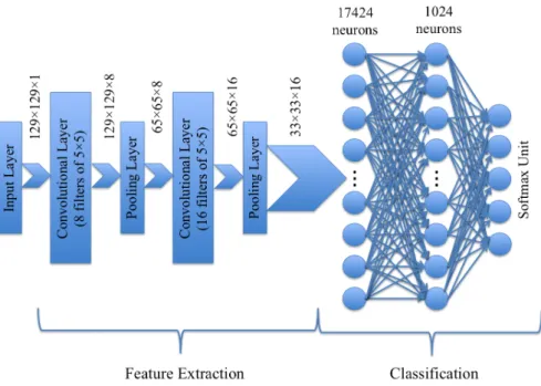
narrow-band spectrogram with 25 ms Hamming window . . . 28 4.2 The baseline architecture of the CNN used in the current study to
classify speech utterances based on their emotional states. . . 30 5.1 The performance accuracy of the CNN models that were trained
and tested on the EMODB database . . . 32 5.2 The color-map confusion matrix of the CNN with the highest
per-formance and 100 training epochs on the EMODB database . . . . 33 5.3 The color-map confusion matrix of the CNN with the highest
5.4 The color-map confusion matrix of the CNN with the highest per-formance and 4000 training epochs on the EMODB database . . . . 35 5.5 A comparison between the CNN performance on the original EMODB
database and the augmented EMODB database . . . 36 5.6 The average performance accuracy of the CNN models over 5 folds
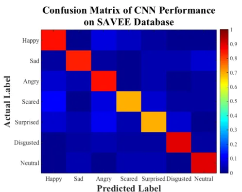
trained and tested on the SAVEE database . . . 38 5.7 The color-map confusion matrix of the CNN with the highest
per-formance and 100 training epochs on the SAVEE database . . . 39 5.8 The color-map confusion matrix of the CNN with the highest
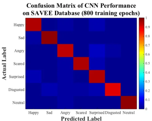
per-formance and 800 training epochs on the SAVEE database . . . 40 5.9 The color-map confusion matrix of the CNN with the highest
per-formance and 4000 training epochs on the SAVEE database . . . . 40 5.10 A comparison between the CNN performance on the original SAVEE
database and the augmented SAVEE database . . . 42 5.11 The average performance accuracy of the CNN models over 5 folds
trained and tested on the EMOVO database . . . 44 5.12 The color-map confusion matrix of the CNN with the highest
per-formance and 100 training epochs on the EMOVO database . . . . 45 5.13 The color-map confusion matrix of the CNN with the highest
per-formance and 800 training epochs on the EMOVO database . . . . 45 5.14 The color-map confusion matrix of the CNN with the highest
per-formance and 4000 training epochs on the EMOVO database . . . . 46 5.15 A comparison between the CNN performance on the original EMOVO
database and the augmented EMOVO database . . . 47 5.16 The average performance accuracy of the CNN models over 5 folds
trained and tested on the BTNRH database . . . 49 5.17 The color-map confusion matrix of the CNN with the highest
5.18 The color-map confusion matrix of the CNN with the highest per-formance and 800 training epochs on the BTNRH database . . . 51 5.19 The color-map confusion matrix of the CNN with the highest
per-formance and 4000 training epochs on the BTNRH database . . . . 51 5.20 A comparison between the CNN performance on the original
BT-NRH database and the augmented BTBT-NRH database . . . 53 5.21 The average performance accuracy of the CNN models over 5 folds
trained and tested on the all-inclusive, language-independent database with 100 training epochs . . . 54 5.22 The average performance accuracy of the CNN models over 5 folds
trained and tested on the all-inclusive, language-independent database with 400 training epochs . . . 55 5.23 The color-map confusion matrix of the CNN with 4000 training
iterations on the all-inclusive, language-independent database . . . 57 5.24 Convolutional neural network with 100 training epochs vs human
on the EMOVO database . . . 61 5.25 Convolutional neural network with 4000 training epochs vs human
List of Tables
4.1 A summary of the databases used in the current study . . . 26 4.2 Class labels of each database . . . 29 5.1 The summary of the architectures and the results of the experiments
ran on the EMODB database . . . 32 5.2 The numerical confusion matrix of the CNN with the highest
per-formance and 100 training epochs on the EMODB database . . . . 34 5.3 The numerical confusion matrix of the CNN with the highest
per-formance and 800 training epochs on the EMODB database . . . . 35 5.4 The numerical confusion matrix of the CNN with the highest
per-formance and 4000 training epochs on the EMODB database . . . . 36 5.5 The summary of the architectures and the results of the experiments
ran on the SAVEE database . . . 37 5.6 The numerical confusion matrix of the CNN with the highest
per-formance and 100 training epochs on the SAVEE database . . . 39 5.7 The numerical confusion matrix of the CNN with the highest
per-formance and 800 training epochs on the SAVEE database . . . 41 5.8 The numerical confusion matrix of the CNN with the highest
per-formance and 4000 training epochs on the SAVEE database . . . . 41 5.9 The summary of the architectures and the results of the experiments
ran on the EMOVO database . . . 43 5.10 The numerical confusion matrix of the CNN with the highest
5.11 The numerical confusion matrix of the CNN with the highest per-formance and 800 training epochs on the EMOVO database . . . . 46 5.12 The numerical confusion matrix of the CNN with the highest
per-formance and 4000 training epochs on the EMOVO database . . . . 47 5.13 The summary of the architectures and the results of the experiments
ran on the BTNRH database . . . 48 5.14 The numerical confusion matrix of the CNN with the highest
per-formance and 100 training epochs on the BTNRH database . . . 50 5.15 The numerical confusion matrix of the CNN with the highest
per-formance and 800 training epochs on the BTNRH database . . . 52 5.16 The numerical confusion matrix of the CNN with the highest
per-formance and 4000 training epochs on the BTNRH database . . . . 52 5.17 The summary of the architectures and the results of the experiments
ran on the all-inclusive, language-independent database . . . 56 5.18 The numerical confusion matrix of the CNN with 4000 training
iterations on the the all-inclusive, language-independent database . 56 5.19 A comparison between the classification accuracy by human
lis-teners and the convolutional neural network using the EMODB database with 100 training epochs . . . 58 5.20 A comparison between the classification accuracy by human
lis-teners and the convolutional neural network using the EMODB database with 4000 training epochs . . . 59 5.21 A comparison between the convolutional neural network
imple-mented in the current study and some previous models . . . 60 5.22 The numerical confusion matrix of the Human performance on the
EMOVO database . . . 62 5.23 A comparison between the classification accuracy by human
listen-ers and the convolutional neural network with 100 training epochs using the EMOVO database . . . 62
5.24 A comparison between the classification accuracy by human listen-ers and the convolutional neural network with 4000 training epochs using the EMOVO database . . . 63 5.25 F1-scores of each emotion for all language-dependent and all-inclusive
models with 100 training epochs . . . 65 5.26 F1-scores of each emotion for all language-dependent and all-inclusive
models with 800 training epochs . . . 65 5.27 F1-scores of each emotion for all language-dependent and all-inclusive
Chapter 1
Introduction
The past several decades have witnessed a wealth of studies on understanding the human brain and building systems that mimic human intelligence [1, 2, 3, 4, 5, 6]. The human brain is an intricate organ that has been a lasting inspiration for research in Artificial Intelligence (AI). The neural networks of human brain are strongly competent to learn high-level abstract concepts from experiencing low-level information processed by sensory periphery. Learning language, understand-ing speech, and recognizunderstand-ing faces are some examples that manifest the remarkable power of the human brain in learning high-level concepts. The main goal of AI is to develop intelligent systems that are able to generate rational thoughts and behaviors similar to human thought and performance [1]. There are a variety of study fields that are considered as the sub-fields of AI. Computer vision, natu-ral language processing, automated reasoning, robotics, machine listening, and machine learning are some of these major areas in AI research.
Developing machines that interact with humans by understanding speech pave the way for building systems that are equipped with human-like intelligence. Speech is the most natural and convenient way by which humans communicate, and understanding speech is one of the most intricate processes that human brain performs. Automatic speech recognition (ASR) has been an active field of AI research aiming to generate machines that communicate with people via speech [7, 8]. The early ASR systems mainly focused on the linguistic properties of speech to understand spoken utterances [9, 10, 11, 12]. Speech is an information-rich sig-nal that contains paralinguistic information as well as linguistic information.
Iden-tity, gender, intention, mood, and emotion are some key paralinguistic information that are conveyed by speech and they were less investigated by the classical ASR framework [13]. The human brain employs all linguistic and paralinguistic infor-mation to understand the underlying meaning of the utterances and have effective communication. In fact, any deficit in the perception of paralinguistic features has an adverse effect on the quality of communication. It has been argued that children who are not able to understand the emotional states of the speakers de-velop poor social skills and in some cases they show psychopathological symptoms [14, 15]. This highlights the importance of recognizing the emotional states of speech in effective communication. Hence, developing machines that understand paralinguistic information such as emotion is imperative for establishing a clear, effective, and human-like communication.
Emotion recognition has been the subject of research for years. Detection of emotion from facial expressions and biological measurements such as heart beats or skin resistance formed the preliminary framework of research in emotion recog-nition [16]. More recently, emotion recogrecog-nition from speech signal has received growing attention. The traditional approach toward this problem was based on the fact that there are relationships between acoustic features and emotion. In other words, emotion is encoded by acoustic and prosodic correlates of speech sig-nals such as speaking rate, intonation, energy, formant frequencies, fundamental frequency (pitch), intensity (loudness), duration (length), and spectral characteris-tic (timbre) [13, 17]. There are a variety of machine learning algorithms that have been examined to classify emotions based on their acoustic correlates in speech utterances. Hidden Markov models (HMM), Gaussian mixture models, nearest neighborhood classifiers, linear discriminant classifiers, artificial neural networks, and support vector machines are some examples that have been widely used to classify emotions based on their acoustic features of interest [13, 17, 18, 19, 20]. The performance of these classifiers mostly depends on the feature extraction tech-niques and the features that are considered salient for a specific emotion. Given
the fact that the acoustic correlates of emotion in speech signals vary across speak-ers, gendspeak-ers, language, and cultures [13], there is no universal agreement on the acoustic correlates of emotions [21, 22]. This results in a myriad of “hand-crafted” features depending on the speech corpus. Using deep learning models is one sen-sible approach to tackle this problem.
Speech emotion recognition is inherently a multimodal process. Although speech modality conveys a large portion of the emotional information, it is not sufficient for recognizing affective states of humans in daily-life situations. Other modalities such as visual or linguistic modality also contribute to convey neces-sary information required for recognizing emotions. That is, in addition to speech, people use other paralinguistic cues such as facial expression, body language, se-mantic, or context to identify emotions in others. In fact, it has been debated that 55% of the message is conveyed by body language when people communicate with one another [23]. We limited our study to speech modality and have not consid-ered other modalities. As a result, the databases that were acted by actors were used in the current study because the emotions were expressed with exaggera-tion by actors, which potentially compensates for the lack of informaexaggera-tion provided by other modalities. This allows us to explore the effectiveness of deep learning models with greater control compared with using daily-life utterances. On the other hand, the broad availability of the acted speech benchmarks in the speech community enables us to compare our work with previously explored models. In the current study, we investigated the capability of convolutional neural networks in classifying speech emotions using acted speech databases within and across four different languages: German, Italian, British English, and American English. The specific contribution of this study is using wide-band spectrograms instead of narrow-band spectrograms as well as assessing the effect of data augmentation on the accuracy of our models across widely-used benchmark databases. Our results revealed that wide-band spectrograms and data augmentation equipped CNNs to achieve the state-of-the art accuracy and surpass human performance.
The remainder of this thesis is organized as follows. Chapter 2 briefly reviews the previous work related to the current study. Chapter 3 explains the basic machine learning concepts that are essential to understand the experiments con-ducted in the current work. Chapter 4 describes the experimental setup including the architecture of the networks that were implemented, and the databases that were administered in this study. Chapter 5 delineates the results and discusses the outcomes. Chapter 6 summarizes the current study and suggests potential work for future.
Chapter 2
Related Work
Deep learning is a modern machine learning technique that emerged to deal with big databases and complex systems. The advent of deep learning brought with it a wave of novel algorithms that diminished the need for “hand-crafted” fea-tures prior to classification [24]. That is, deep learning models can learn low-level features from training data in their lower layers and build high-level representa-tion in the upper layers based upon the proceeding layers. As a result, the deep learning models are able to extract the features automatically. Recently, a rapid growth has been observed in using deep learning models to classify speech emo-tions. The efficacy of deep learning models in speech emotion recognition has been examined during last years in various studies. Stuhlsatz et al. [25] compared the performance of a Generalized Discriminant Analysis (GerDA) based on deep neu-ral networks (DNNs) with support vector machines (SVM) on classifying speech utterances using their emotional dimensions such as arousal and valence [26]. In a specific preprocessing procedure, the static acoustic features were extracted and fed into the classifiers as the input data. Their results showed that the DNN highly outperformed the SVM in detection of emotional dimensions of speech utterances. Li et al. [27] compared the performance of the hybrid deep neural network-hidden Markov model (DNN-HMM) classifier with the hybrid Gaussian mixture model-hidden Markov model (GMM-HMM) classifier in speech emotion recognition. The DNN in the DNN-HMM was used to extract the discriminative features that were later used by the HMM to classify speech emotions. Their results showed that the DNN-HMM outperformed the GMM-HMM in classifying speech emotions. Mao
et al. [28] used convolutional neural networks, which are a specific kind of deep learning models, to automatically learn discriminative features from the narrow-band spectrograms of speech signals. Subsequently, they used an SVM to classify the features learned by CNN. Their results demonstrated a superior performance in learning high-level discriminative features from the low-level spectrographic representation of the speech signals. Fayek et al. [29] implemented a deep neural network (DNN) to classify speech emotions. The one-second narrow-band spec-trograms of the speech signals were used as the input of the DNN. Their results showed an improvement over classic machine learning algorithms. Zheng et al. [30] implemented a convolutional neural network to learn discriminative features from narrow-band log-spectrograms of speech signals. Similar to previous stud-ies, their results showed a performance improvement over the methods that used hand-crafted features to classify speech emotions. Trigeorgis et al. [31] proposed an end-to-end deep learning model in which they combined a convolutional neural network with a recurrent neural network. Recurrent neural networks (RNNs) are sequence models that deal with sequential data such as speech, text, or video [32]. Trigeorgis et al. [31] took advantage of the spatial resolution of the CNNs and the temporal resolution of the RNNs to extract discriminative features of emotions from the raw data without any preprocessing; that is, they used the raw audio signals as the inputs of their model. Their results also confirmed the efficacy of the deep learning models in learning salient features to recognize affective states of humans using their speech utterances. Recently, Papakostas et al. [33] assessed the capability of deep convolutional neural networks in classifying speech emotions using publicly available databases. In doing so, they compared the performance of deep neural models with SVM classifiers. Their results manifested the supe-rior performance of the deep neural networks over SVM classifiers in recognizing emotional states of the speech sounds. Specifically, Papakostas et al. [33] devel-oped convolutional neural networks with four convolutional layers, each followed by a max-pooling layer, and two fully connected layers. The stochastic gradient
descent (SGD) algorithm was used to train the networks with 5000 training iter-ations. The models were tested and withing and across languages using F1-score. In addition, dropout technique and data augmentation were employed to combat overfitting the training data. To augment training data, background noise with three different levels of signal to noise ratio was added to speech signals. The 250 ×250 narrow-band spectrogram images of the speech signals were fed into the deep neural networks as the input. In our work, we also examined the effi-cacy of convolutional neural networks in decoding emotions in speech signal. Our work differs from the work by Papakostas et al. [33] from several aspects. For in-stances, we used wide-band spectrogram images as the input of the convolutional neural networks in lieu of the narrow-band spectrogram images; also, we used a different learning algorithm and slightly different data augmentation. Further, we developed convolutional neural networks with significantly smaller number of hyperparameters and notably faster than the models developed by Papakostas et al. [33]. Above all, our convolutional neural networks outperformed the previ-ous models including the work by Papakostas et al. [33]. Prior to diving into the details of our work, next chapter reviews some basic concepts in machine learning and deep learning.
Chapter 3
Deep Artificial Neural Networks
Machine learning is an area of study in Computer Science and Artificial In-telligence. It primarily focuses on developing algorithms that can automatically learn a task or a skill, and gain knowledge by experience such as observing train-ing data. Subsequently, it is desirable that machine learntrain-ing algorithms generalize well their learned knowledge from these observations to new, unseen data. In doing so, different learning strategies such as supervised learning, unsupervised learning, or reinforcement learning can be employed. In what follows, we give a brief introduction on supervised learning as it has been applied in the current study. To learn about other types of learning, we refer the reader to Mitchell et al. [34], Bishop [35], Suton and Barto [36], and James et al. [37].
In supervised learning, the training data incorporate the desired response, called labels; that is, for each observation (training sample or instance), there is a corresponding label. The goal of learning is to predict the label of each training/test instance as correctly as possible. Classification is one example of supervised learning wherein the machine learning algorithm learns to classify the input data into two or more categories. To do so, the algorithm learns the discrim-inant features or attributes across different categories or classes based on observing training data. These features are later used to classify new test input data. Arti-ficial neural networks (ANNs) are one well-known instance of supervised learning algorithms although some ANNs can be trained by unsupervised learning [38]. ANNs are inspired by the way biological neural networks, such as human central nervous system, work. That is, they consist of a highly interconnected processing
units, called neurons. ANNs are the basic building blocks of deep learning, which is a strong modern machine learning technique. In fact, deep learning models are ANNs with a plethora of neurons and layers. Deep learning models have achieved remarkable successes in various machine learning applications such as classifica-tion. The key concept that makes deep learning models efficacious is their ability to learn complex features out of simple features [24]. That is, the first layers of deep learning models represent simple and basic features of the training data. The deeper layers build a complex representation by using these low-level features. This ability of building high-level features out of low-level features can potentially reduce the amount of preprocessing required for extracting hand-crafted features before designing classifiers. In the current study, we have implemented a deep learning model, called convolutional neural network, to classify emotional states of speech signals.
This chapter provides background knowledge that is necessary to understand the experimental setup (Chapter 4) and results (Chapter 5) of the current work. The remainder of this chapter is organized as follows. In Section 3.1, we introduce the multi-layer perceptron network, which is a popular ANN architecture. In Section 3.2, we introduce the convolutional neural network, which is a well-known and effective deep learning model, especially in the field of speech and image processing. Finally, in Section 3.3, we describe k-fold cross-validation, which is a commonly used model assessment technique to evaluate the performance of machine learning models.
3.1 Multi-layer Perceptron Networks
The network architecture is one of the factors that characterizes artificial neural networks (ANNs). It determines the way neurons, the basic processing units, are connected to one another. The multi-layer perceptron (MLP) is a long-established ANN architecture that is composed of neurons called linear threshold units (LTUs) [38]. Figure 3.1 illustrates a linear threshold unit. As demonstrated, an LTU
receives weighted inputs from different neurons (here from three neurons) and computes the linear combination of the inputs as z = w1x1 +w2x2 +w2x2 +b,
where b is the bias term. Then, a step function (e.g., Heaviside function H(x) or Sign functionsgn(x)) is applied on the linear combination to generate the output as y = f(z) where f is a step function. If the weighted sum is greater than a threshold value (which is affected by the bias term), the LTU will generate an output.
Figure 3.1: Linear threshold unit. It processes the inputs by computing the linear combination of the inputs and applying a step function.
Generally, an MLP incorporates one input layer, one or more LTU layers (called hidden layers), and one output layer. The information flows from the input layer (lower level) toward the output layer (higher level). That is why they are called feedforward artificial neural networks. The input layer represents the values of one training sample in different dimensions. This can be the amplitude of an audio signal at different sampling points or the intensity of an image at different pixels. The input is usually denoted as a vector ~x whose length indicates the number of dimensions (e.g., the number of sampling points in an audio signal or the number of pixels in an image). The output is either a real number, y, or a vector,~y, which shows the label of the input. An MLP is mainly configured as the layers of the neurons denoted as l[0], l[1], l[2], . . . , l[n], l[n+1], where l[0] is the input layer, l[1], l[2], . . . , l[n]are the n hidden (LTU) layers, andl[n+1] is the output layer. Every neuron within the layerl[1j≤]j≤(n+1)(all layers except the input layer) directly receives the weighted input from every neuron within a layer that is one level low,
i.e., l[j−1]. Figure 3.2 demonstrates an MLP with one hidden layer where W 1 and
W2 are matrices associated with the values that weight the inputs of the neurons
in the hidden layer and the output layer, respectively. The vectors b~1 and b~2 are
the weights associated with bias terms.
Figure 3.2: Multi-layer perceptron. W1 and b~1 denote the weight matrix and the
bias vector associated with the input layer. W2 and b~2 are the weight matrix and
the bias vector associated with the hidden layer.
In fact, the weight matrices (W1 and W2) and the bias vectors (b~1 and b~2)
are the parameters of interest. That is, the network learns to classify the input data by adjusting the values of these parameters. There are several learning techniques that can find the optimum values of these parameters. Backpropagation is one example of these learning methods that has been widely used to train MLP networks. The basis of the backpropagation algorithm is gradient descent, which is briefly introduced in the next section.
3.1.1 Gradient Descent
Searching for the optimum values of the weight parameters can be viewed as an optimization problem. Having the error function or loss function, the goal is to find the parameters of interest in a way that minimize the error function. There are several ways to define the error function. Equation 3.1 displays a well-established error function called sum of squared errors [34] where W, d, and D stand for weights, one training instance, and all training data, respectively. As
shown, the squared of error between the actual label (t~d) and the predicted label (y~d) is summed over all training data. The goal is to search the weight space for the values that minimize this function.
E(W) = 1 2
X
d∈D
(t~d−y~d)2. (3.1)
Gradient descent is a common optimization algorithm that is used to minimize the error function. Suppose we have a linear unit that computes the weighted sum of its inputs as follows:
z =w1x1+w2x2+· · ·+wpxp+b =w~ ·~x+b, (3.2)
where b, w~, ~x, and z are the bias term, weight vector, the input vector, and the output of the linear unit, respectively. This unit’s error function is
E(w~) = 1 2
X
d∈D
(td−yd)2. (3.3)
Gradient descent, which is an iterative technique, begins with a random initial values of the weight parameters and updates the weights in the opposite direction of the gradient of the error function as presented in equation 3.4 [34]
wi =wi−η ∂E ∂wi
, (3.4)
wherewi is the weight associated with theith dimension of the input and ηis the learning rate that determines the step of updates.
The backpropagation algorithm employs gradient descent to find the local min-ima of the error function of the multi-layer perceptron (MLP) networks. The error function of the MLP networks is not convex as it is in a linear unit. As a result, finding global minima is not guaranteed. Since we do not have access to the out-put of the hidden neurons, the backpropagation algorithm takes advantage of the chain rule of calculus and computes the contribution of hidden neurons to the
output error to update the weights associated with the hidden layers [24, 38]. It should be noted that the step function of the MLP networks poses challenges for taking the derivative with respect to the weights. Therefore, the step function is replaced with the sigmoid function, σ(x) = 1+1e−x ,which is differentiable. For
more detail, we refer the reader to [34, 24, 38].
There are several variants of gradient descent such as gradient descent with momentum [39] or root mean square propagation (RMSprop) [40] that increase the rate of convergence. Gradient descent with momentum uses an exponentially decaying weighted average of gradients instead of gradients to update the weights. That is, the gradient across the number of iterations can be viewed as a time-series signal, ∂E∂w(t), where t stands for the number of iterations. The gradients can be replaced with the exponentially weighted average of gradients as vt = βvt−1+ (1−β)∂E∂w(t), wherev0 = 0 andβ ∈[0,1], to update the weights. RMSprop
optimization computes the exponentially decaying weighted average of the squared gradient, m(t) = βmt−1 + (1− β)(∂w∂E(t))2, where m0 = 0 and β ∈ [0,1], and
use its square root to scale the learning rate as η0 = √η
m(t). These variants of
gradient descent can be used to smooth out the oscillation around local optima and increase the rate of convergence. Adam algorithm introduced by Kingma and Ba [41] is another gradient-based optimization algorithm that combines the merits of gradient descent with momentum and RMSprop optimization to minimize the loss function [42]. That is, it employs the first order momentum as in gradient descent with momentum and the second-order momentum as in RMSprop optimization to update the weights. The name of this algorithm roots from “adaptive moment estimate”. This algorithm is very effective and has been widely used in deep learning models.
3.2 Convolutional Neural Networks
Convolutional neural networks (CNNs) are one of the most popular deep learn-ing models that have manifested remarkable success in the research areas such as
object recognition [43], face recognition [44], handwriting recognition [45], speech recognition [46], and natural language processing [47]. The term convolution comes from the fact that convolution—the mathematical operation—is employed in these networks. Generally, CNNs have three fundamental building blocks: the convo-lutional layer, the pooling layer, and the fully connected layer. Following, we describe these building blocks along with some basic concepts such as softmax unit, rectified linear unit, and dropout.
3.2.1 Convolutional Layer
Convolutional layers in CNNs use convolution instead of multiplication to com-pute the output. As a result, the neurons in the convolutional layers are not con-nected to all the neurons in their preceding layers. This architecture is inspired by the fact that neurons of the visual cortex have local receptive field [48, 49]. That is, the neurons are specialized to respond to the stimuli limited to a specific location and structure. As a result, using convolution introduces sparse connec-tivity and parameter sharing to CNNs, which decreases the number of parameters in deep neural networks drastically.
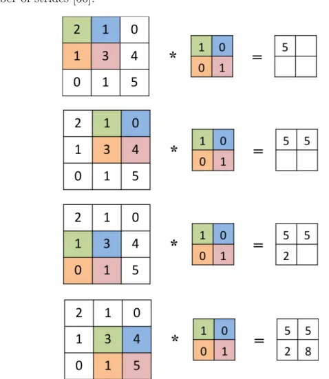
Figure 3.3 demonstrates the convolution of a kernel, which is a 2×2 matrix, with a one-channel 3×3 image. The output is a volume of 2×2×1. Generally, the size of output is (nh−f+ 1)×(nw−f+ 1)×nf, wherenh is the height of the input,nw is the width of the input, andnf is the number of kernels. The depth of the kernel is determined by the depth of the input. For the example demonstrated in Figure 3.3, the depth of the input is nc = 1. As a result the depth of kernel is 1. Also, the depth of the output is 1 since there is only one kernel. As can be seen, each output neuron is the weighted sum of the input neurons within the corresponding receptive field, which introduces sparse connectivity in CNNs. Further, the kernel is shared across the layer, which introduces parameter sharing in CNNs. The step by which the kernel slides along the input is called stride. In our example (Figure 3.3), the stride is s = 1, which means that the kernel shifts
one step over the image. It should be noted that the input volume shrinks after each convolutional layer. To avoid this decrease, we can pad the outer edge of the input with zero. Overall, the height and width of the output is determined by
nh+2p−f s + 1×nw+2p−f s
+ 1, wherepis the number of zero padding andsis the number of strides [50].
Figure 3.3: The convolution of a 3×3 image by a 2×2 kernel with a stride of 1. The local filtering that happens in convolutional layers allows detecting differ-ent basic low-level features of interest and generating various feature maps. The deep layers use these feature maps to construct the high-level representation of the inputs.
3.2.2 Pooling Layer
The second important building block of CNNs is a pooling layer. This layer is used to make the outputs less sensitive to the local variation in the inputs.
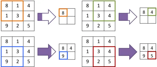
This invariance to small local translation can decrease the spatial resolution and lead to underfitting in some applications. When accurate spatial features are not required, pooling can improve the performance of CNNs in extracting the features of interest. Further, pooling can reduce overfitting since it decreases the number of dimensions and parameters [24]. In a sense, pooling takes subsamples from the outputs [38]. Similar to convolutional layers, pooling layers use a kernel (a rectangular receptive field) to apply an aggregation function such as maximum, average, L2-norm, or weighted average to summarize the values of the neurons within the pooling kernel. To have a pooling layer in CNNs, we need to determine the size of pooling kernels, the step of shifting, and the number of padding. Figure 3.4 depicts max pooling over a 3×3 matrix where the size of pooling kernel is 2×2 and the kernel shifts one pixel over the matrix (i.e., stride of 1).
Figure 3.4: Pooling of a 3×3 image using a 2×2 kernel with a stride of 1; the maximum value of each window is supsampled.
3.2.3 Fully Connected Layer
A typical CNN consists of several convolutional layers where each convolutional layer is followed by a pooling layer. The last building block of CNNs is the fully connected layer, which is basically a traditional MLP. This component is used to either make a more abstract representation of the inputs by further processing of the features or classify the inputs based on the features extracted by preceding
layers [51].
3.2.4 Softmax Unit
A softmax unit is usually used as the output of the fully connected layer. A softmax unit employs softmax function (normalized exponential) to represent the probability distribution of k classes. In fact, softmax function is a generalization of the sigmoid function, σ(z) = 1
1+e−z = e z
1+ez, which manifests the probability
distribution of two possible classes [24]. Equation 3.5 displays the softmax function
softmax(~z)i = ezi
Pk j=1ezj
, (3.5)
where ~z is the output of the k-way softmax unit, softmax(~z)i is the probability that the input instance is in class i, and zi is the ith element of the vector ~z.
3.2.5 Rectified Linear Unit
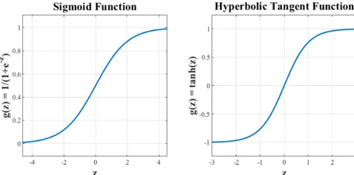
The activation functions have been the linchpin of artificial neural networks (ANNs). That is, they incorporate nonlinearity into ANNs, which makes ANNs an effective tool to learn complex models. Sigmoid function g(z) =σ(z) = 1+1e−z
and hyperbolic tangent function g(z) = tanh(z) = 2σ(2z)−1 are two popular activation functions, especially in traditional ANNs (see Figure 3.5).
Figure 3.5: Sigmoid activation function and hyperbolic tangent activation func-tion.
One disadvantage of these functions is that they saturate for zs that have high absolute values, which adversely affects the gradient-based learning. To overcome this shortcoming, the rectified linear unit (ReLU)—g(z) = max(z,0)—can be employed as an activation function [24]. Figure 3.6 shows the ReLU function. Despite its nonlinearity property around z = 0, it behaves linear for z > 0 and
z <0. ReLU functions provide a compromise between the nonlinearity, needed to
learn complex models, and linearity, needed to facilitate gradient-based learning. As a result, ReLU functions are widely used as the activation function in deep learning models. In convolutional layers of CNNs, ReLU functions are applied on the feature maps before subsampling of the pooling layers. The main drawback of the ReLU functions is the zero output for thezs with negative value. This problem is known as the dying ReLUs [38]; that is, the output of the neurons becomes zero during the training and remains zeros. As a result, the neurons become ineffective. To eliminate this problem, a variant of ReLU function, named leaky ReLU has been introduced, ReLUα(z) = max(αz, z), where α determines the slope of the ReLU function for z < 0 [52, 38]. Previous research has shown that using leaky ReLU may increase the likelihood of overfitting the training data for the small number of the training instances [38]. This is because the number of parameters will increase, which consequently increases the sensitivity of the network to the nuisance variances.
3.2.6 Cross-entropy
The cross-entropy between labels, provided by training data, and the outputs, generated by softmax function, is used as a measure of the loss function. The cross entropy is
H(l, s) = H(l) +DKL(l||s), (3.6) wherel denotes the true probability distribution of the labels andsdenotes the es-timated probability distribution of the labels by softmax unit. H(l) is the entropy of l and DKL is the Kullback-Leibler divergence of s froml.
In communication theory, entropy is a measure of information that reflects the degree of uncertainty or choice in a system; that is, a greater randomness or uncertainty is associated with a larger degree of freedom of choice that indicates the greater information in a system [53]. The definition of entropy is
H =X
x∈X
p(x) log 1
p(x), (3.7)
whereX is a random variable with probability distribution ofpand possible values of {x1, x2, . . . , xn}.
The Kullback-Leibler divergence measures how well the classifier estimateslby using s [54]. The more s diverges from l, the more the predictions are uncertain. The objective of learning is to set the parameters such that they minimize the cross-entropy orDKL. The discrete entropy can be written as
H(l, s) = −X
x
l(x) logs(x). (3.8)
In convolutional neural networks (CNNs) where softmax unit is used to esti-mate the probability distribution of the classes, the cross-entropy is considered a better loss function than the mean squared error (MSE) [24] mostly because MSE is more effective in the regression problems when the outputs have real continuous value.
3.2.7 Mini-batch Learning
The large number of training examples in deep learning models hampers the speed of learning and poses challenges for computing resources. The idea of using mini batches of examples from the training set seeks to ameliorate the problem of the enormity of the data [24]. That is, the network is trained over several batches instead of one batch of training data for each iteration. Specifically, the optimization problem occurs on several error subfunctions instead of one single error function. Mini-batch learning lies between two extremes of batch learning and stochastic learning. In batch learning, to which we alluded earlier, all training instances are used to train the model for each iteration. However, in stochastic learning, every instance is used separately to form an error function to train the model for each iteration. The primary benefit of stochastic and mini-batch learning is preserving time and computing resources. However, they never converge to the global optimum; instead, the stochastic or mini-batch algorithms either approach or fluctuate around the global optimum [42, 38]. The mini-batch learning is more accurate than stochastic learning since it takes a larger portion of training data into consideration while optimizing the error functions. Albeit, stochastic learning can escape local optima easier than mini-batch leaning [38]. The size of mini batches is usually set to 64, 128, 256, 512, or 1024 in deep leaning models such as convolutional neural networks (CNNs) [42].
3.2.8 Dropout
Variance and bias are two competing properties of gradient-based learning [37]. The estimated underlying model of a system can be changed depending on the training set used for learning. Variance is a concept that refers to these changes. Ideally, the goal is to have a model that is a general representative of the system behavior and, hence, it is less sensitive to the the specific training set. Models with high variance follow the noise-induced changes in training set and overfit the training data. Generally, complex models suffer from high variance. On the other
hand, the models built over the assumptions that simplify the real behavior of the system have high bias. These models fail to capture the underlying complexity of the system and underfit the training data.
There is a high risk of overfitting the training set (high variance) in deep learn-ing models due to the excessive amount of trainlearn-ing data and model parameters of deep neural networks. In traditional machine learning, there is a trade-off be-tween variance and bias; that is, decreasing variance leads to increasing bias and vice versa. However, training deep architectures, along with big training sets, has resolved this long-standing variance-bias dilemma. So long as the deep networks are properly regularized, the variance can be reduced without hurting the bias [42].
Models with high variance perform well on the training set, but they are un-successful to generalize well on the test set. L1-norm regularization andL2-norm regularization are two common traditional approaches to remedy overfitting. That is, the objective function incorporates weight decay into the the loss function as shown below for L1-norm regularization and L2-norm regularization [42, 24], re-spectively J(w, b) = 1 m m X i=1 L(l(i), s(i)) + λ 2mkwk1, (3.9) J(w, b) = 1 m m X i=1 L(l(i), s(i)) + λ 2mkwk 2 2, (3.10)
wheremis the number of training data,L denoted the loss function such as cross-entropy or mean squared error (MSE), l(i) is the true label of the ith training instance, s(i) is the predicted label of the ith training instance, w denotes the parameters of interest, andλ is a hyperparmeter that controls the strength of the regularization. Incorporating the regularization term constraints the optimization to the small values of w. This may yield weight assignment to a smaller number of features, which consequently decreases the complexity of the model.
powerful regularization technique to reduce overfitting. Dropout is a strong and highly effective algorithm that regulates the deep neural networks by randomly omitting the neurons in the hidden layers during training. The neurons are omitted with an assigned probability, say,p[55]. The outputs and the error function of the networks can be cast as random variables. In other words, dropout approximates bagged ensemble training where training data is used to train multiple networks [24]. Therefore, the output of the network with dropout can be viewed as an average ensemble of multiple networks with different architectures [38]. Baldi and Sadowski [56] have proven that the expected value of the error function of the network with dropout includes a regularization term similar to weight decay in L1-norm and L2-norm regularization. Further, they have argued that the highest level of regularization can be achieved when the hidden neurons are omitted with the probability of p= 0.5.
3.2.9 Data Augmentation
Deep learning models strive for data because their actual power is magnified when they are trained with large data sets [57]. In fact, increasing the size of train-ing set has been an effective way to fight overfitttrain-ing and to improve generalizability of deep learning models [24]. However, acquiring new data is an expensive, time-consuming endeavor. To tackle the data collection problem, data augmentation— which is a regularization technique—is employed to artificially synthesize new training data and increase the size of training sets [38]. Recent years have wit-nessed a major success of data augmentation in several machine learning tasks, especially in classification [24, 58, 59, 60, 43, 61]. In supervised learning, data aug-mentation includes transformation techniques to which the classifier of interest is invariant. That is, the class label of data is not affected by data augmentation. For instance, rotation of images for object recognition task or embedding speech signals in background noise for speech emotion recognition task effectively boosts the size of training sets without vitiating the labels of instances.
3.3 k-Fold Cross-Validation
Cross-validation is a model assessment technique that is used to evaluate the performance of machine learning models. In this technique, the data is randomly divided intok distinct non-overlapping subsets, or folds with approximately equal sizes. The first fold is used as the validation set to evaluate the performance of the model whereas the remaining k−1 folds are used as the training set to train the model. This procedure is repeated k times wherein the kth fold is treated as the validation set and the remainder of the folds are treated as the training test for each kth trial. Ultimately, the average of performance accuracy across these k test sets is used to estimate the performance of the model [37, 38, 24].
Chapter 4
Experimental Setup
In the current study, we implemented convolutional neural networks (CNNs) to classify speech utterances based on their emotional contents. In addition to three widely used benchmarks for recognition of emotion from speech utterances [62, 63, 64], we used a private database to train and evaluate our models. We used TensorFlow (an open-source library written in Python and C++ [65]) as the pro-gramming framework to implement our CNN models. This chapter describes the experimental setup of the current work. The first section introduces the databases administered in our study (summarized in Table 4.1). The second section explains the preprocessing procedure. The third section describes the training and test setup used to train and evaluate our models. Finally, this chapter ends by intro-ducing the baseline architecture of the CNNs implemented in the current work.
4.1 Databases
4.1.1 EMODB: German Database
The Berlin Database of Emotional Speech (EMODB)1 is a public German
speech database that incorporates audio files with seven emotions: happiness, sad-ness, anger, fear, disgust, boredom, and neutral [62]. The German utterances were recorded by five men and five women (9 of them had passed an acting schooling) producing 10 utterances for each emotion. Twenty listeners evaluated the emo-tional labels of the utterances. The sentences had emoemo-tionally neutral contents and were recorded with a sampling rate of 48 kHz and downsampled to 16 kHz.
1
The sentences with recognition accuracy of greater than 60% were chosen for fur-ther analysis. This lead to 71 happy, 62 sad, 127 angry, 69 scared, 46 disgusted, 81 bored, and 79 neutral speech utterances for a total of 535 speech samples.
4.1.2 SAVEE: British English Database
The Surrey Audio-Visual Expressed Emotion (SAVEE)2 is a public British English speech database that has audio files with seven emotion labels: happi-ness, sadhappi-ness, anger, fear, disgust, surprise, and neutral [63]. Four English male actors generated 15 utterances for each emotion. Three of these utterances were common among all emotions. Two of them were emotion specific. The remain-ing utterances were generic sentences that were different across six emotions but neutral. The three common and two emotion specific sentences of each emotion were used to record neutral emotions. The sampling rate of all recordings was 44.1 kHz. Overall, there are 60 utterances for each emotion except neutral and 120 utterances for neutral for a total of 480 utterances. We randomly selected 60 utterances from 120 neutral utterance. Therefore, we used 420 utterances of this database.
4.1.3 EMOVO: Italian Database
EMOVO3 is a public Italian speech database that includes audio files with
seven emotion labels: happiness, sadness, anger, fear, disgust, surprise, and neutral [64]. Six Italian actors (three female and three male) generated 14 utterances for each emotion. The sentences were either emotionally neutral or nonsense and were consistent across emotions. All sentences were recorded with sampling rate of 48 kHz. There are 84 utterances for each emotion for a total of 588 utterances.
2
http://personal.ee.surrey.ac.uk/Personal/P.Jackson/SAVEE/
3
4.1.4 BTNRH: American English Database
BTNRH is a private American English speech database that was developed in Auditory Prosthesis and Perception Laboratory at Boys Town National Research Hospital, furnished by Dr. Monita Chatterjee (personal communication). It has audio files with five emotional states: happiness, sadness, anger, fear, and neutral. We used utterances generated by 12 American speakers (seven female and five male) in our experiments. The speakers uttered 12 sentences with each of the 5 emotion states. We used 144 utterances for each emotion for a total of 720 utter-ances. The sentences were emotionally neutral and were recorded with sampling rate of 44.1 kHz.
4.1.5 All-Inclusive: Language-Independent Database
All databases were integrated to form a language-independent database across German, Italian, British English, and American English languages. In doing so, we first identified the shared emotion classes across all languages. All databases had happy, sad, angry, scared, and neutral speech utterances. Therefore, the bored and disgusted speech instances were removed from the EMODB database, and the surprised and disgusted speech examples were removed from the SAVEE and EMODB databases while the speech sounds with joint emotion classes were preserved. This led to the all-inclusive database with 5 emotional states.
Table 4.1: A summary of the databases used in the current study—the number of utterances for each emotional state and the total number of utterances.
Database Happy Sad Angry Scared Neutral Disgusted Surprised Bored Total
EMODB 71 62 127 69 79 46 - 81 535
SAVEE 60 60 60 60 60 60 60 - 420
EMOVO 84 84 84 84 84 84 84 - 588
BTNRH 144 144 144 144 144 - - - 720
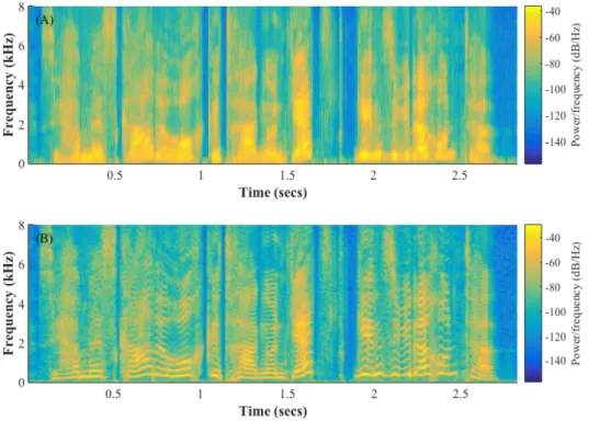
4.2 Preprocessing
In order to have a consistent sampling rate across all databases, all utterances were resampled and filtered by an antialiasing FIR lowpass filter to have frequency rate of 16 kHz prior to any processing. All audio utterances were then converted into spectrograms. A spectrogram is an image that displays the variation of en-ergy at different frequencies across time. The vertical axis (ordinate) represents frequency and the horizontal axis (abscissa) represents time. The energy or in-tensity is encoded either by the level of darkness or by the colors. There are two general types of spectrograms: wide-band spectrograms and narrow-band spectro-grams. Wide-band spectrograms has a higher time resolution than narrow-band spectrograms. This property enables the wide-band spectrograms to show individ-ual glottal pulses. In contrast, narrow-band spectrograms have higher frequency resolution than wide-band spectrograms. This feature enables the narrow-band spectrograms to resolve individual harmonics [66, 67]. Figure 4.1 depicts the wide-band and narrow-wide-band spectrogram images of a speech utterance.
Considering the importance of vocal fold vibration, along with the fact that glottal pulse is associated with one period of vocal fold vibration [66], we decided to convert all utterances into wide-band spectrograms. In doing so, the length of Hamming windows were set to 5 ms with 4.4 ms overlap. The number of DFT points was set to 512. Also, we discarded the frequency information greater than 4 kHz from spectrograms since frequencies below 4000 Hz are sufficient for speech perception in many situations [68]. In pilot studies, eliminating energy above 4000 Hz improved the performance of the algorithms. This gave 129 frequency points. All spectrogram images were, first, resized to have 129 ×129 pixels and, then, z-normalized to have zero mean and standard deviation close to one.
Figure 4.1: (A) Wide-band spectrogram with 5 ms Hamming window; (B) narrow-band spectrogram with 25 ms Hamming window.
4.3 Training and Test Sets
Our models were trained and evaluated using 5-fold cross-validation. That is, the data were partitioned into 5 folds. The first fold was used as a test set whereas the other folds were used to train our models. Then, the second fold was used to test our models while the remainder of the folds were used for training, and so on. To reduce overfitting and the adverse effect of small size of databases, the data sets were augmented by adding white Gaussian noise with +15 signal to noise ratio (SNR) to each audio signal either 10 times or 20 times. The SNR is defined as 10 log10(Pspeech
Pnoise ), where P is the average power of the signal. The data
augmentation resulted in two types of data sets used to train our models: data sets with 10 times augmentation (10x) and data sets with 20 times augmentation (20x). We used the original data without noise to test our models. The augmented data were used only for training. Finally, the labels of the training and the test data were encoded as one-hot vectors. Table 4.2 shows the class labels of each
database. The number of training epochs was varied between 100 to 4000. The favorable training epoch was set to 100 due to the computation and time expenses.
Table 4.2: Class labels of each database. Stimulus Type
Emotion EMODB SAVEE EMOVO BTNRH
happy 1 1 1 1 sad 2 2 2 2 angry 3 3 3 3 scared 4 4 4 4 bored 5 - - -surprised - 5 5 -disgusted 6 6 6 -neutral 7 7 7 5 4.4 Architecture
The baseline architecture of the deep neural network that was implemented in the current study was a convolutional neural network with two convolutional layers and one fully connected layer with 1024 hidden neurons. Depending on the number of classes, either a 5-way or a 7-way softmax unit was used to estimate the probability distribution of the classes. Every convolutional layer was followed by either a max-pooling or average-pooling layer. Rectified Linear Units (ReLU) were used in convolutional and fully connected layers as activation functions to introduce nonlinearity to the model. The initial kernel size of convolutional layers was set to 5×5 with stride of 1. The initial number of kernels was set to 8 and 16 for the first and the second convolutional layers, respectively. The kernel size of pooling layers was set to 2×2 with stride of 2. Cross-entropy was used as the loss function and the Adam optimizer was employed to minimize the loss function over the mini batches of the training data. The size of the mini batches was set to 512. The number of training iteration was 100. The networks developed in this study took between 30 minutes to 2 days to be trained using Graphics Processing Units (GPUs). Broadly speaking, GPUs are used instead of CPUs to accelerate the speed
Figure 4.2: The baseline architecture of the CNN used in the current study to classify speech utterances based on their emotional states.
of computation since GPUs have several cores and can handle a large number of concurrent threads. We used the Crane cluster of the Holland Computing Center at University of Nebraska-Lincoln to run our experiments. Further, we incorporated the dropout algorithm into the fully connected layer to improve the performance of our networks whenever the symptoms of overfitting were diagnosed. Figure 4.2 illustrates the fundamental building blocks of the CNN model in the current work.
Chapter 5
Results & Discussion
We ran several language-dependent, gender-independent experiments on each database. We embarked on our study by implementing the baseline CNN archi-tecture introduced in Chapter 4. Subsequently, we modified the hyperparameters such as the size of convolution kernels and the deletion probability of the dropout algorithm hing on the performance of the models. This chapter aims to present the results of these experiments and to discuss the outcomes.
5.1 Results
5.1.1 EMODB: German Database
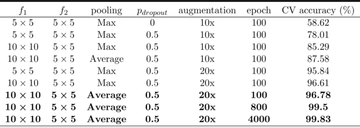
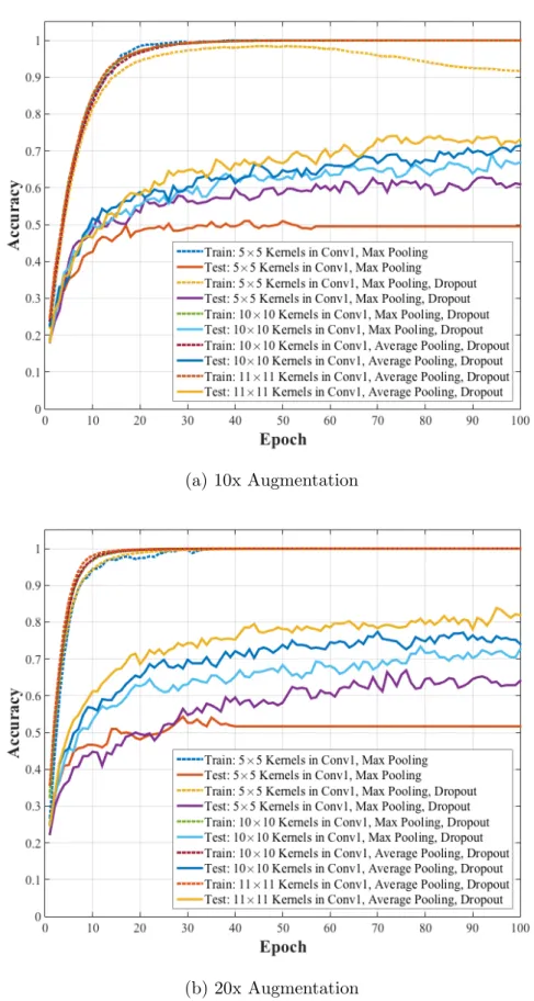
We ran several experiments on the EMODB database. In all experiments, our networks learned the training data with accuracy 100%. However, the accuracy on the test data was varied across different architectures. Table 5.1 summarizes the architectures and their corresponding accuracy on the test data. The accuracy on the test data is the average of accuracy of the test data across the 5 folds of the cross-validation evaluation. Figure 5.1 demonstrates the accuracy of the CNN models over training and test for each iteration of learning.
As demonstrated, the first significant boost in the performance of our network occurred when dropout was employed. Applying dropout increased the test accu-racy from 58.62% to 78.01%. Increasing the window size of the first convolutional layer from 5×5 to 10×10 also improved the performance of the network. Fur-ther, using average pooling instead of max pooling enhanced the performance. The second significant boost occurred by increasing the number of augmentation
Table 5.1: The summary of the architectures and the results of the experiments ran on the EMODB database; f1 is the size of the kernels in the first convo-lutional layer, f2 is the size of the kernels in the second convolutional layer, pdropout is the deletion probability of dropout, epoch denotes the number of training iterations, and CV stands for cross-validation.
f1 f2 pooling pdropout augmentation epoch CV accuracy (%)
5×5 5×5 Max 0 10x 100 58.62 5×5 5×5 Max 0.5 10x 100 78.01 10×10 5×5 Max 0.5 10x 100 85.29 10×10 5×5 Average 0.5 10x 100 87.58 5×5 5×5 Max 0.5 20x 100 95.84 10×10 5×5 Max 0.5 20x 100 96.61 10×10 5×5 Average 0.5 20x 100 96.78 10×10 5×5 Average 0.5 20x 800 99.5 10×10 5×5 Average 0.5 20x 4000 99.83
Figure 5.1: The performance accuracy of the CNN models that were trained and tested on the EMODB database.
from 10 times augmentation to 20 times augmentation. This increase yielded a test accuracy of 95.84%. Increasing the window size of the first convolutional layer enhanced the performance from 95.84% to 96.61%. Using average pooling in lieu of max pooling changed the performance from 96.61% to 96.78%. Taken together, the highest performance was associated with the architecture with 10×10 kernels
in the first convolutional layer, 5×5 kernels in the second convolutional layer, average pooling, dropout with p= 0.5, and training data with 20x augmentation. Figure 5.2 illustrates the color-map confusion matrix for the architecture with the highest accuracy after 100 training epochs. Table 5.2 shows the corresponding numerical values of this color map. As can be seen, the network classified un-seen angry utterances with 100% accuracy. Bored and disgusted emotions were classified with the poorest accuracy compared with other emotions.
Figure 5.2: The color-map confusion matrix of the CNN with the highest perfor-mance and 100 training epochs on the EMODB database.
Moreover, the architecture with the highest performance, as given in Table 5.1 (10×10 kernels in the first convolutional layer, 5×5 kernels in the second convolutional layer, average pooling, dropout with p = 0.5), was trained and tested with 800 and 4000 training epochs. The results indicated an improvement in the test accuracy as the number of training epochs increased. Figures 5.3 and 5.4 illustrates the color-map confusion matrices of the CNN with 800 and 4000 training epochs, respectively. Tables 5.3 and 5.4 show the corresponding numerical values of these color maps. As demonstrated, increasing the number of training improved the performance of the model on the test data.
Table 5.2: The numerical confusion matrix of the CNN with the highest perfor-mance and 100 training epochs on the EMODB database. The diagonal numbers show the percent of each class that was correctly identified. The off-diagonal numbers displays the percent of each class that was incorrectly identified as other classes.
Predicted Labels
happy sad angry scared bored disgusted neutral
Actual Lab els happy 95.77 0 4.23 0 0 0 0 sad 0 96.77 0 0 0 0 3.23 angry 0 0 100 0 0 0 0 scared 0 0 2.9 97.10 0 0 0 bored 2.47 0 0 0 92.59 1.23 3.70 disgusted 0 0 2.17 2.17 0 93.48 2.17 neutral 0 0 0 1.27 1.27 0 97.47
Figure 5.3: The color-map confusion matrix of the CNN with the highest perfor-mance and 800 training epochs on the EMODB database.
Further, to underline the effect of data augmentation on the performance of the CNN model, the CNN architecture with the highest performance (10×10 kernels in the first convolutional layer, 5×5 kernels in the second convolutional layer, average pooling, dropout with p = 0.5) was trained on the original EMODB database and the augmented (20x) EMODB database, separately. Figure 5.5 depicts the accuracy of the CNN models on the test data. As demonstrated, the CNN that
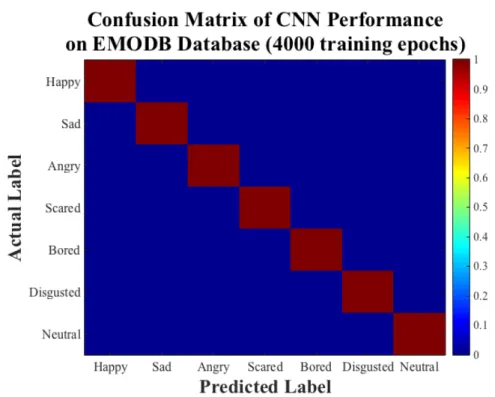
Figure 5.4: The color-map confusion matrix of the CNN with the highest perfor-mance and 4000 training epochs on the EMODB database.
Table 5.3: The numerical confusion matrix of the CNN with the highest perfor-mance and 800 training epochs on the EMODB database. The diagonal numbers show the percent of each class that was correctly identified. The off-diagonal numbers displays the percent of each class that was incorrectly identified as other classes.
Predicted Labels
happy sad angry scared bored disgusted neutral
Actual Lab els happy 98.59 0 1.41 0 0 0 0 sad 0 100 0 0 0 0 0 angry 0 0 100 0 0 0 0 scared 0 0 0 100 0 0 0 bored 0 0 0 0 100 0 0 disgusted 0 0 4.35 0 0 95.65 0 neutral 0 0 0 0 0 0 1
was trained on the original database classified the test data with accuracy of approximately less than 55% whereas the CNN that was trained on the augmented database classified the same test data with accuracy close to 99.5%. This highlights the crucial role of data augmentation in enhancing the CNN performance.
Table 5.4: The numerical confusion matrix of the CNN with the highest per-formance and 4000 training epochs on the EMODB database. The diagonal numbers show the percent of each class that was correctly identified. The off-diagonal numbers displays the percent of each class that was incorrectly identified as other classes.
Predicted Labels
happy sad angry scared bored disgusted neutral
Actual Lab els happy 100 0 0 0 0 0 0 sad 0 100 0 0 0 0 0 angry 0.79 0 99.21 0 0 0 0 scared 0 0 0 100 0 0 0 bored 0 0 0 0 100 0 0 disgusted 0 0 0 0 0 100 0 neutral 0 0 0 0 0 0 100
Figure 5.5: A comparison between the CNN performance on the original EMODB database and the augmented EMODB database.
5.1.2 SAVEE: British English Database
Table 5.5 summarizes the experiments performed on the SAVEE database. The outcomes reveal that the network with 11×11 kernels in the first convolutional layer, 5×5 kernels in the second convolutional layer, average pooling, dropout with p= 0.5, and 20 times augmentation of the training data had the best performance