Pattern Recognition Using Spiking Neural Networks

(1)

Scholarship at UWindsor

Electronic Theses and Dissertations Theses, Dissertations, and Major Papers

7-7-2020

Amir Javid Talaei

University of Windsor

Follow this and additional works at: https://scholar.uwindsor.ca/etd

Recommended Citation Recommended Citation

Talaei, Amir Javid, "Pattern Recognition Using Spiking Neural Networks" (2020). Electronic Theses and Dissertations. 8402.

https://scholar.uwindsor.ca/etd/8402

This online database contains the full-text of PhD dissertations and Masters’ theses of University of Windsor students from 1954 forward. These documents are made available for personal study and research purposes only, in accordance with the Canadian Copyright Act and the Creative Commons license—CC BY-NC-ND (Attribution, Non-Commercial, No Derivative Works). Under this license, works must always be attributed to the copyright holder (original author), cannot be used for any commercial purposes, and may not be altered. Any other use would require the permission of the copyright holder. Students may inquire about withdrawing their dissertation and/or

(2)

Using

Spiking Neural Networks

By

Amir Javid Talaei

A Thesis

Submitted to the Faculty of Graduate Studies

through the Department of Electrical and Computer Engineering

in Partial Fulfillment of the Requirements for

the Degree of Master of Applied Science

at the University of Windsor

Windsor, Ontario, Canada 2020

c

(3)

Using

Spiking Neural Networks

By

Amir Javid Talaei

APPROVED BY:

A. Edrisy

Department of Mechanical, Automotive & Materials Engineering

E. Abdel-Raheem

Department of Electrical & Computer Engineering

M. Ahmadi, Advisor

Department of Electrical & Computer Engineering

(4)

I hereby certify that I am the sole author of this thesis and that no part of this thesis has been published or submitted for publication.

I certify that, to the best of my knowledge, my thesis does not infringe upon any-one’s copyright nor violate any proprietary rights and that any ideas, techniques, quotations, or any other material from the work of other people included in my the-sis, published or otherwise, are fully acknowledged in accordance with the standard referencing practices. Furthermore, to the extent that I have included copyrighted material that surpasses the bounds of fair dealing within the meaning of the Canada Copyright Act, I certify that I have obtained a written permission from the copyright owner(s) to include such material(s) in my thesis and have included copies of such copyright clearances to my appendix.

I declare that this is a true copy of my thesis, including any final revisions, as approved by my thesis committee and the Graduate Studies office, and that this thesis has not been submitted for a higher degree to any other University or Institution.

(5)

Deep learning believed to be a promising approach for solving specific problems in the field of artificial intelligence whenever a large amount of data and computation is available. However, tasks that require immediate yet robust decisions in the presence of small data are not suited for such an approach. The superior performance of the human brain in specific tasks like pattern recognition in comparison to traditional neural networks convinced neuroscientists to introduce a biologically plausible model of the neuron, which is known as spiking neurons. In opposition to conventional neuron, spiking neurons use a short electrical pulse known as a spike to transfer the information. The complexity and dynamic of these neurons allow them to perform complex computational tasks. However, training a spiking neural network does not follow the rule of conventional ANN, and we need to devise new methods of training that are compatible with the unsupervised nature of these networks. This thesis aims to investigate the unsupervised approaches of training spiking networks using spike time-dependent plasticity (STDP) and assess their performance on real-world machine learning applications like handwritten digit recognition.

(6)

to

My Parents

for Their Unconditional Love

and Support

(7)

I wish to express my sincere gratitude to my advisor, Dr. Majid Ahamdi. His continuous support, encouragement, and patience have been instrumental to this thesis.

I am also inclined to express my profound appreciation to my committee members, Dr. Esam Abdel-Raheem of the Department of Electrical and Computer Engineering and Dr. Afsane Edrisy of the Department of Mechanical, Automotive & Materials Engineering for their insightful comments during the development of this thesis. Special gratitude belongs to my family, my parents, and my brother, for providing me with incredible support and encouragement throughout the years of my study. This work would not have been possible without their sacrifice and continued care.

(8)

DECLARATION OF ORIGINALITY iii ABSTRACT iv DEDICATION v ACKNOWLEDGMENTS vi LIST OF TABLES x LIST OF FIGURES xi

LIST OF ABBREVIATIONS xiii

1 INTRODUCTION 1

1.1 Introduction . . . 1

1.1.1 Why SNN? . . . 4

1.2 Dynamic of a Biological Neuron . . . 5

1.3 Models of a Single Neuron . . . 9

1.3.1 McCulloch-Pitts Model . . . 9

1.3.2 Hodgkin-Huxley Model . . . 10

1.3.3 Integrate-And-Fire Models . . . 13

1.3.4 Izhikevich Model . . . 18

1.3.5 Spike Response Model(SRM) . . . 21

1.4 Neural Coding . . . 24

(9)

1.4.3 Sine Wave Encoding . . . 27

1.4.4 Spike Density Code . . . 27

1.5 Synaptic Plasticity . . . 28

1.5.1 Mathematical Formulation of Hebb’s Rule . . . 29

1.5.2 Pair-based Models of STDP . . . 30

1.5.3 Triplet model of STDP [38] . . . 33

1.6 Unsupervised Learning [15] . . . 34

1.6.1 Rate model learning . . . 35

1.6.2 STDP Learning Equations . . . 38

1.7 Summary . . . 39

1.8 Outline of the thesis . . . 40

2 SURVEY OF RELEVANT LITERATURE 41 2.1 A Review of Supervised Learning in SNN . . . 41

2.2 Unsupervised Learning in SNN . . . 43

2.3 Summary . . . 46

3 PROPOSED SNN FOR IMAGE CLASSIFICATION 48 3.1 Introduction . . . 48 3.2 Network Architecture . . . 49 3.2.1 MNIST dataset . . . 50 3.2.2 Input Encoding . . . 51 3.2.3 Neuron Model . . . 52 3.2.4 Learning Rule . . . 55 3.2.5 Parameters Tuning . . . 60 3.3 Simulation Results . . . 61 3.4 Conclusion . . . 67

4 HANDWRITTEN DIGIT RECOGNITION USING STDP 69 4.1 Introduction . . . 69

(10)

4.2.1 Neuron and Synapse Model . . . 70 4.2.2 Network Architecture . . . 71 4.2.3 Learning Rule . . . 72 4.2.4 Adaptive Threshold . . . 76 4.2.5 Training . . . 77 4.3 Results . . . 78 4.4 Conclusion . . . 84 5 CONCLUSION 87 5.1 Future Works . . . 88 BIBLIOGRAPHY 90 VITA AUCTORIS 96

(11)

1.1 Comparison of the SNN and other machine learning techniques [25]. . 5 3.1 Comparison of three SNN. . . 68 4.1 Parameters for simulation of the SNN. . . 84 4.2 Performance of different methods on the MNIST dataset. . . 85

(12)

1.1 A model of Spiking Neuron [37]. . . 3

1.2 Diagram of a Neuron [10]. . . 6

1.3 Scheme of synaptic transmission [3]. . . 8

1.4 McCulloch and Pitts Model. . . 10

1.5 Hodgkin-Huxley Model. . . 11

1.6 Electrical properties of the Integrate-And-Fire neuron. . . 14

1.7 Potential of the cell membrane (bottom) when a step current (top) injected to the membrane. . . 16

1.8 Izhikevich neuron model. . . 19

1.9 Comparison of different neuron models [24]. . . 21

1.10 Spike Response Model [16]. . . 23

1.11 Illustration of the temporal coding principle [37]. . . 25

1.12 Definition of mean firing rate by temporal average. . . 26

1.13 Spike-Timing Dependent Plasticity (schematic) [42]. . . 31

1.14 The triplet STDP rule with local variables [16]. . . 34

2.1 Unsupervised learning rule in SNN proposed in [35]. . . 43

2.2 Architecture of the memristor-based SNN proposed in [39]. . . 45

2.3 Architecture of the Diehel & Cook network [13]. . . 46

3.1 Proposed SNN architecture for image classification. . . 50

3.2 Sample images from MNIST test set. . . 51

(13)

input spike train. . . 55

3.5 STDP curve of (Eqn.3.6). . . 57

3.6 Neuron B (Winner) sends lateral signals to Neuron A and C. . . 59

3.7 Receptive field of output neurons. . . 62

3.8 Membrane potential of the neuron 4 in response to input images. . . . 63

4.1 Two-layer SNN based on the architecture proposed in [40]. . . 71

4.2 Schematic of the STDP based on equation (Eqn. 4.5) and (Eqn. 4.4). 73 4.3 STDP weight change based on pre ans postsynaptic spike timing [43]. 74 4.4 Encoding the input image to Poisson-distributed spike train. . . 77

4.5 Raster diagram of SNN network with 400 output neurons. . . 79

4.6 Selectivity of the neuron. . . 80

4.7 2D receptive field of the network with 625 output neuron. . . 81

4.8 2D receptive field of the SNN network with 400 output neuron. . . 82

(14)

AI Artificial Intelligence ANN Artificial Neural Network

EPSP Excitatory Postsynaptic Potential GA Genetic Algorithm

IF Integrate And Fire Neuron IPSP Inhibitory Postsynaptic Potential LIF Leaky Integrate And Fire Neuron LTD Long Term Depression

LTP Long Term Potentiation MLP Multilayer Perceptron PSP Postsynaptic Potential SNN Spiking Neural Network SOM Self Organizing Map SRM Spike Response Model

STDP Spike Timing Dependent Plasticity WTA Winner Takes All Strategy

(15)

INTRODUCTION

1.1

Introduction

Recent advances in the field of artificial intelligence and machine learning affected various aspects of human life. With the emergence of self-driving cars, the prolifer-ation of virtual assistants, and highly intelligent search engines, we feel the presence of AI in our life more than ever.

One of the milestones in the history of artificial intelligence happened when Hinton and Osindero [20] published their work about deep neural networks. In their paper, they proposed a method to pre-train deep neural networks one layer at a time and lay the foundation for the field of deep learning, which finds its way for widespread industrial use.

In comparison with the first generation of neural network with linear activation func-tion, the second generation (deep networks) consist of neurons with non-linear activa-tion funcactiva-tion (sigmoid funcactiva-tion) which can perform much more complicated machine

(16)

learning tasks than the previous generation.

However, comparing the performance of the best deep neural networks with human-level performance highlights the need for a more biologically plausible model of a neuron, which known as spiking neuron. Spiking neural networks are a class of neuron models developed to mimic the behavioral dynamics of the biological neurons. The ability to exhibit the dynamics of one or more variable states enabled them to capture phenomena not seen in artificial neural networks. These spiking neurons communicate by sending short period, high amplitude pulse of activity referred to as spikes [1]. In the spiking neurons, the output of activation function computed by each neuron not only depends on the value of its inputs but also on the timing of input arrival. Such temporal coding allows a spiking neuron to surpass its sigmoidal counterpart in terms of flexibility of computational tasks. The dynamics of a spiking neuron influenced by the incoming spikes determines the condition and time for sending spikes.

(17)

Figure 1.1: A model of Spiking Neuron [37].

Figure 1.1 illustrates a model of spiking neuron; neuron Nj generates an action po-tential (spike) whenever the weighted sum of incoming PSP (postsynaptic popo-tential) approaches the threshold value. The diagram below shows the changes in membrane potentials of Nj in response to four incoming spike.

There are different types of dynamical SNN models with varying levels of sophisti-cation. However, training a spiking neural network is not as straightforward as the conventional neural networks with the backpropagation algorithm, and the question of training a spiking neural network is still wide open. Recent studies have shown that precise spike encoding broadly used by the brain, providing a higher transformation speed and metabolic efficiency [46].

(18)

1.1.1

Why SNN?

SNN hold exceptional qualities that make them superior in a few aspects in compar-ison with traditional machine learning techniques [25]:

• Effective modeling of processes that include various time scales • Event prediction

• Parallel information processing • Compact information processing

• Low energy consumption on neuromorphic hardware

Dharmendra Modha manager and lead researcher of the Cognitive Computing group at IBM highlights the significance of brain-inspired computing as follow:

“The goal of brain-inspired computing is to deliver a scalable neural network substrate while approaching fundamental limits of time, space, and energy”.

Table 1.1 illustrates a comprehensive comparison of the spiking neural networks with other machine learning methods over different inclinations.

(19)

Method/Features Statistical Method

ANN SNN

Information Scalars Scalars Spike sequences

Data

Representation

Scalars, vectors Scalars, vectors Whole TSTD patterns

Learning Statistical, limited Hebbian rule STDP

Dealing with TSTD Limited Moderate Excellent

Parallel Computation

Limited Moderate Massive

Hardware Support Standard VLSI Neuromorphic VLSI

Table 1.1: Comparison of the SNN and other machine learning techniques [25].

1.2

Dynamic of a Biological Neuron

Although neurons are only one of many brain cells, they have attracted more attention than other brain cells because of their fundamental role in computational operations. The fundamental function of a neuron is simple: the neuron receives input signals from other neurons via connections called Synapses, and if the input signals excite them sufficiently, they will fire an action potential (spike) that propagates through synapses to other neurons.

Neurons consisted of three main parts: the dendrite, the soma, and the axon. Den-drites considered as the receiver of input signals, and neurons receive input current via their dendrites. This input current then transmitted to the main body of the cell, called the soma. When a neuron generates an action potential, it sends current down its axon, causing neurotransmitters to release at the synapses, which are connections

(20)

from a neuron’s axon to the dendrites of other neurons. This neurotransmitter release causes the flow of dendritic currents in other connected neurons.

The main body of the neuron called soma. From a computational perspective, this is where all the incoming currents from dendrites integrated. The process of producing an action potential also occurs in the soma.

Figure 1.2: Diagram of a Neuron [10].

When a neuron is in resting state, the soma has a negative potential called the resting potential and controlled by ion pumps that maintain a particular concentration of ions (mostly sodium Na+, potassium K+, and calcium Ca2+) inside the cell. The incoming current from dendrites causes the cell membrane to depolarize.

(21)

connection. The single output of this neuron is an action potential (spike) which emits whenever the membrane voltage reaches a threshold.

Whenever the potential in the soma becomes high enough, it starts to trigger sodium channels, which allow sodium ions to enter the cell and further depolarizing it. The process continues until the electrical gradient of the sodium channel opposes the chemical gradient of imbalance in sodium charge inside and outside of the cell. This process causes a considerable change in membrane potential and alters the membrane potential from a negative to a positive charge.

The considerable depolarization of the membrane potential triggers the potassium channels and let them reach out of the cell and eventually repolarize it. At the same time, the sodium channels become inactivated. The open potassium channels finally bring the cell to a potential lesser than its resting potential, which called the hyperpolarized state. Here process continues for a short while in which the neuron is not capable of generating spikes, which called the absolute refractory period.

(22)

Figure 1.3: Scheme of synaptic transmission [3].

Figure 1.3 demonstrates the schematic of synaptic transmission in a neuron. In part (a), the neuron is ready to transmit a signal. Part (b) presents the sending of spike upon arrival of the spike into the terminal. Here, calcium appears as a second messenger hence triggering a cascade of biochemical responses.

The difference in ionic concentrations inside the cell membrane is considerably small during a single spike, but throughout many spikes, the ion pumps require to maintain the proper concentrations of sodium and potassium. The immediate depolarization of membrane potential triggers the sodium channel in axonal parts and generates a voltage wave that moves down the axon. Eventually, this voltage wave triggers the synaptic vesicles proximate to the ends of the axon and let them release neurotrans-mitters.

(23)

1.3

Models of a Single Neuron

1.3.1

McCulloch-Pitts Model

In 1943, McCulloch and Pitts published their famous model of a neuron, which known as the logic threshold unit. The computational ability of their two-state neural model presented in [31]. In such a model, the neuron can be either in an active or inactive state. Whenever the current value of the neuron surpasses a predefined value known as the threshold, neuron’s state will change from inactive to active. They also used the structure of inhibitory synapses in which a neuron connected to inhibitory synapses is not able to become active by itself.

One of the great results of their works is that we can implement some of the most fundamental logical gates using their model. This property attracted much attention among computer scientists and lay the foundation for what we know as Von Neumann architecture.

However, the McCulloch and Pitts model does not represent the full functionality of an actual neuron and has its limitations. The input to this neuron model is in binary form, and inputs with real value do not apply to this neuron. In addition to this, the McCulloch and Pitts model is only able to perform linearly separable functions, and we can not implement linearly non-separable functions like XOR using this neuronal model.

Figure 1.4 demonstrates the McCulloch-Pitts neural model with a set of inputx1,x2,

...,xnand one outputy. The output is in binary form. We can represent the function of the neuron using (Eqn.1.1) and (Eqn.1.2).

(24)

Figure 1.4: McCulloch and Pitts Model. g = n X i=1 xiwi (1.1) y=f(g) (1.2)

Where w1, w2, ..., wn are weight values normalized in range (0,1). The function f expressed as f(x) = h(x−T), where h is the Heaviside step function, and T is the threshold value.

1.3.2

Hodgkin-Huxley Model

In 1952, following a comprehensive set of experiments on the giant axon of the squid, Hodgkin and Huxley presented their mathematical model for describing the dynam-ics of a neuron. In their model, action potentials are the result of currents that pass through ion channels. They used differential equations to describe the dynamic behavior of these ion channels. Their model immediately acknowledged as a ground-breaking achievement in neuroscience society and eventually led to the Nobel Prize

(25)

in 1963 [21].

For decades, neuroscientists successfully used this model to simulate the actual op-eration in the human brain. However, the computational cost is the main barrier for simulating a network consisting of a large number of neurons.

Hodgkin and Huxley described the dynamic of a neuron using three different ion channels consisted of the potassium channel, sodium channel, and a channel that handles other types of ions known as the leakage channel. The cell body acts as a semipermeable membrane and allows only specific ions to pass through it. The flow of those ions across the membrane defines the internal potential concerning the potential outside of the cell [15].

Figure 1.5: Hodgkin-Huxley Model.

The model explained by the aid of Figure 1.5. The cell membrane separates the interior of the cell from the extracellular environment. This membrane, therefore, can think of as a capacitor in an electrical circuit. If we introduce the input current I(t) into the cell, it may increase the charge of capacitors or leak into ionic channels of the cell membrane. Each ion channel outlined in the Figure 1.5 using a resistor. The resistance of sodium, potassium and leakage channel indicated by respectively

(26)

RNa,RK, and R. We denote the potential across this membrane by u. Three current

components of their model formulated, as shown in (Eqn.1.3). The channels char-acterized by their respective conductance, which denoted by gNa, gK and gL. The

value of conductance for sodium and potassium is at its maximum level when those channels are open.

X

k

Ik =gNam3h(u−ENa) +gKn4(u−EK) +gL(u−EL) (1.3)

ENa, EK, and EL are respectively, the reversal potential of sodium, potassium, and

leakage channel. We can express the activation of each channel of the model in terms of voltage-dependent transition ratesα and β as:

˙ m=αm(u) (1−m)−βm(u)m ˙ n=αn(u) (1−n)−βn(u)n (1.4) ˙ h=αh(u) (1−h)−βh(u)h

The terms m andh are controlling variables for the sodium channel while the potas-sium channels constrained by the term n. Here ˙m, ˙n and ˙h are respectively the derivative of the m, n and h with respect to the time.

The differential equations in (Eqn.1.5) determine how the gating variables m, n and h evolving over time. This gating variable defines the probability for which a particular channel is open since most of the time; one of these channels is blocked.

(27)

˙

x=− 1 τx(u)

[x−x0(u)], (1.5)

Hodgkin-Huxley model can successfully describe the dynamic of the squid neuron (their experimental subject); however, experiments confirm that there are other kinds of electrophysiological properties in cortical neurons of the vertebrates, which need additional channels to explain the behavior of the neuron sufficiently. Detailed mod-els of these types of neurons developed over the years, however, the computational demand of these models made the Hodgkin-Huxley model the first choice for neuro-scientific investigations.

1.3.3

Integrate-And-Fire Models

Integrate-and-Fire models represent action potentials as events in which if the volt-age ui(t) (which comprises the summed effect of all inputs) reaches a threshold ϑ, the neuron fires a spike. The shape of the action potentials is not of the highest importance in this model. To describe the dynamics of the neuron, integrate and fire models use two separate components; first, an equation that defines the evolu-tion of the membrane potentialui(t); and second, a mechanism for generating action potentials [16].

(28)

Figure 1.6: Electrical properties of the Integrate-And-Fire neuron.

The variableui represents the membrane potential of neuroni. Usually, the potential is at its resting value urest when there is no incoming input to the cell membrane.

Whenever the neuron receives synaptic input from other neurons, the potential will be different from its resting value.

Figure 1.6 illustrates the electrical properties of the integrate-and-fire neuron. We can link the instantaneous voltage of the cell membrane to the input current from synaptic input using the elementary laws of electricity. Considering the neuron which surrounded by a cell membrane, we can think of it as a capacitor which will charge if a short current pulse I(t) injected into the neuron. Since the insulator is not ideal, we have a slow leakage of potentials through the cell membrane. Finally, we can characterize the cell membrane by a finite leak resistance R.

The basic integrate-and-fire model consists of a capacitor C in parallel with a resistor R and input current I(t).

(29)

Using the law of current and splitting it into two elements we have:

I(t) =IR+IC (1.6) Using Ohm’s law, we can rearrange (Eqn.1.6) to the equation presented below:

I(t) = u(t)−urest

R +C

du

dt (1.7)

Multiplying (Eqn.1.7) by R and using the time constantτm =R C yields the standard form:

τm du

dt =−[u(t)−urest] +R I(t). (1.8) The solution to this differential equation considering the initial condition u(t0) =

urest+ ∆uis in form: u(t)−urest= ∆u exp −t−t0 τm fort > t0. (1.9)

When there is no incoming input to the membrane, the potential exponentially decay to its resting value. The membrane time constant determines the characteristic time of the decay.

(30)

Figure 1.7: Potential of the cell membrane (bottom) when a step current (top) injected to the membrane.

Figure 1.7 demonstrates the smooth reaction of the cell membrane in response to a step input current. We can interpret the result considering the electrical diagram of the RC-circuit in Figure 1.6. Whenever the circuit enters a steady-state, the charge on the capacitor no longer increases, and all the incoming input current should pass through the resistors.

Leaky Integrate-and-fire model [14]

A specific case of integrate and fire neurons which incorporates the notion of leakage channel in membrane potential is leaky integrate and fire model. The leakage channel reflects the diffusion of ions that happens through the membrane when some equi-librium condition is not satisfied in the cell. The differential equation of the leaky integrate-and-fire model represented as:

(31)

dv dt =−

v−veq

τ +I(t) (1.10)

Where veq is the is the equilibrium potential, τ = RC is the time constant of the membrane, and v represents the membrane potential. Integrating the differential equation over an arbitrary input current I we have:

u(t) =η(t−_tˆ_{) +}

Z ∞

0

Θ(t−_tˆ₋_s_{) exp(}₋_s/τ₎_I₍_t₋_s₎_ds _(1.11) Where ˆt is the firing time of the last spike of the neuron, u=v−veq is the potential following the reset after each spike, Θ is the Heaviside step function, and η is the spike shape function which determines the mean shape of spike and represented as:

η(t−ˆt) = (vreset−veq) exp[−(t−ˆt)/τ] (1.12) The leaky integrate and fire is a simplified model of an actual neuron, and it misses several characteristics which neuroscientists have observed when they study neurons in the living brain. However, this model considered as a reliable model for generating spikes since it is surprisingly precise for simulating timed events phenomena [16]. The study suggests that after each spike neurons enter a refractory period during which they are incapable of generating new spikes. In addition to refractoriness, neurons show adaptation, which constitutes over hundreds of milliseconds. We can increase the accuracy of the simple leaky integrate-and-fire model by adding adap-tation and refractoriness to a much higher degree. A simple method to satisfy this property is to consider a dynamic threshold for the neuron model. The neuron thresh-old will increase by constant value θ after each spike and will approach to its stable

(32)

value in the quiescent period. Using the delta function, we can formulate this idea: τadapt d dtϑ(t) = −[ϑ(t)−ϑ0] +θ X f δ(t−t(f)) (1.13)

Wheret(f) =t(1), t(2), t(3)...are firing time of the neuron, andτadaptis the time constant

for adaptation. ϑ(t) and ϑ0 are respectively, membrane and resting potential of the

neuron.

1.3.4

Izhikevich Model

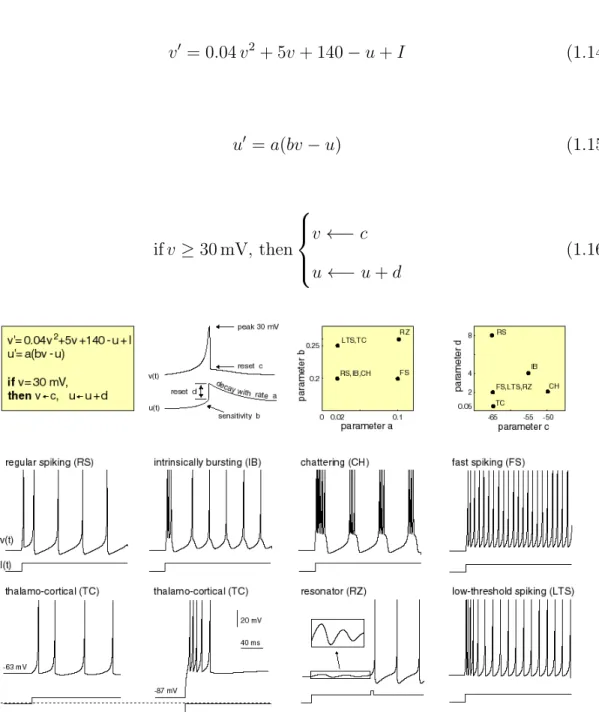
The Izhikevich neuron model is a simplified model of the biological neuron which can describe the dynamic properties of the cell membrane using two distinct differential equations. This model of the neuron is capable of generating various kinds of action potentials observed in biological neurons, which include regular spiking, intrinsically bursting, chattering, and many others [23].

Differential equations in (Eqn.1.14) and (Eqn.1.15) used to describe the Izhikevich model. Here, v is the membrane potential, anduis the membrane recovery variables, which provides negative feedback to v. These two variables are dimensionless. The threshold value set to 30 mV and if the voltage v is larger than the threshold, v and u will reset as (Eqn.1.16). There are four additional dimensionless parameters which are a,b,c, andd. The parametera represents the time scale on which the membrane potential u operates and parameterb represents the sensitivity ofuto fluctuations in v. The parametercused to define the reset potential ofv after a spike and parameter d specifies the reset potential of the variable u after producing an action potential.

(33)

v0 = 0.04v2 + 5v+ 140−u+I (1.14) u0 =a(bv−u) (1.15) ifv ≥30 mV, then      v ←−c u←−u+d (1.16)

Figure 1.8: Izhikevich neuron model.

The input current to the system denoted using parameter I. By adjusting the model parameters a, b, c, and d, we can present different kinds of spiking patterns. Figure

(34)

1.8 demonstrates the ability of the Izhikevich neuron to produce various kinds of ac-tion potentials, including intrinsically bursting (IB), chattering (CH), thalamocortical (TC), and resonator (RZ).

As a consequence of simplification, the Izhikevich model does not reflect the refractory period after generating spikes, which may lead to unrealistic behavior of the neuron under specific situations. A solution to this problem proposed in [44].

To incorporate a refractory period, we need to interrupt the dynamic equation in (Eqn.1.16) whenever v reaches the threshold value at time tf. Therefore we need to modify the (Eqn.1.16) adding a new constraint as shown in (Eqn.1.17) and (Eqn.1.18)

ifv ≥30 mV,andt−tprev ≥∆(abs)

     v ←−c u←−u+d (1.17) else ifv ≥30 thenv ←−30 (1.18)

Possessing a strong biological characteristics and regarding the computational effi-ciency, the Izhikevich neuron is a liable candidate for big network simulations. Figure 1.9 is a comparison between different neuronal model which presented in [24].

(35)

Figure 1.9: Comparison of different neuron models [24].

1.3.5

Spike Response Model(SRM)

There is another approach rather than using the system of differential equations to describe the behavior of the cell membrane, and that is replacing parameters of the model by a (parametric) function of time called filters. Spike response model is a generalized version of the integrate-and-fire model formulated using filters. In contrast to the leaky integrate-and-fire model, this model incorporates the notion of the refractoriness [17].

In the spike response model, the membrane potential denoted by u, which is an essential factor for determining the state of the neuron. In the absence of the input cuurent, the membrane potential is at its resting state urest. Adding a short current

(36)

return to its resting state.

Because of the linear characteristics of the membrane potential below the threshold value, we can express the voltage response h of the membrane to a time-dependent simulating current by (Eqn.1.19).

h(t) =

Z ∞

0

κ(s)Iext(t−s) ds (1.19) Here the functionκ(s) defines the time scale of the voltage response to a short current pulse at time s = 0. Since many ion channels are still open immediately after the spike, the membrane time constant is shorter during that brief period.

We can represent the evolution ofuin regards to incoming spike trains using equation in (Eqn.1.20). Here, the functionη, represents various forms of the action potentials, including depolarizing, hyperpolarizing, and resonating spike-after potential [2].

u(t) =X f η(t−t(f)) + Z ∞ 0 κ(s)Iext(t−s) ds+urest (1.20)

We can rearrange the sum over all past firing times to a convolutional form as in (Eqn.1.21) u(t) Z ∞ 0 η(s)S(t−s)ds+ Z ∞ 0 κ(s)Iext(t−s) ds+urest (1.21)

It is essential to specify that in the SRM model, the threshold value is a time-dependent variable, which differs from the leaky integrate-and-fire model with a fixed threshold (Eqn.1.22). Here we observe an increase in the threshold voltage shortly

(37)

ϑ −→ ϑ(t). (1.22) Whenever the membrane potentialuapproaches the dynamic thresholdϑ(t) from the below, the neuron will generate an action potential (Eqn.1.23).

t=t(f) ⇔ u(t) = ϑ(t) and d[u(t)−ϑ(t)]

dt >0. (1.23)

Figure 1.10: Spike Response Model [16].

Figure 1.10 describes the spike response model (SRM). Input current passes through the filter κ(s) and creates the potential h. If the membrane potential reaches the thresholdϑ, the neuron generates an action potential. After each spike, the membrane threshold increases by θ1. Furthermore, each spike produces a voltage contribution η

to the membrane potential.

The Spike Response Model is incapable of explaining the following properties of the biological neuron:

(38)

• In comparison with the Hodgkin and Huxley model, the spike response model is incapable of describing the biophysics of membrane potential explicitly and therefore performs poorly on the prediction of the individual ion channel. This model considers the effect of several ion channels and predict their spike shape using function η and filter κ. For explaining the behavior of an individual ion channel, Hodgkin and Huxley is a more reliable choice [14].

• As observed in the biological neuron, the action potential delay differs according to the amplitude of the input pulse. We can not see this property in the spike response model. There are another type of neurons, such as the quadratic [28] or exponential integrate-and-fire model [6], which can represent this characteristic.

1.4

Neural Coding

Spiking neural networks employ precise timing of spikes for transferring information, which is significantly different from what we saw in conventional neural networks. Therefore, a different approach for presenting input stimuli to the network required. Various procedures for converting input data to an understandable stimuli for SNN proposed, here we discuss different techniques of neural coding.

1.4.1

Rate vs Temporal Coding

The rate coding refers to encoding the input to a stimulus in terms of firing rate or frequency of action potentials. Contraction of the muscle which is in accordance with the number of spike per time unit, considered as an example of the rate coding in the nervous system [33].

(39)

However, studies suggest that the human brain employs a different procedure for interpreting visual stimuli considering the response time of the visual receptors to these stimuli, which is remarkably short, and no time will remain for ascertaining the average firing rate by the neural system [15]. Though this is not the case in temporal coding, and the timing of individual spikes is equivalently important. Role of precise spike timing for localization of sound in the auditory system is an example of temporal coding [7].

Figure 1.11: Illustration of the temporal coding principle [37].

Figure 1.11 Illustrates the temporal coding procedure for encoding and decoding of real vectors into spike trains. The network supplied by serial of n-dimensional input vectorsX = (x1, x2, ..., xn) which translates to the train of spikes within the successive temporal window. In each time window, a pattern X is temporally coded relative to the timing of the spike emission of the neuron.

To understand the limitation of the current definition of the rate and temporal coding, we should consider the case of two neurons with the same firing rate but different timing for generating spikes. The first neuron generates all its spikes at the beginning of the period and is silent afterward. The second neuron generates its spikes in an

(40)

evenly distributed time during the given period.

To differentiate between these neurons, we should consider the notion of the instan-taneous firing rate. It seems clear that the instaninstan-taneous firing rate is higher for the first neuron at the beginning, however, the second neuron has a fixed instantaneous firing rate for the whole period [12]. If a rapid change in the instantaneous firing rate observed, which contains essential information about input stimuli, the method used called temporal coding.

Figure 1.12: Definition of mean firing rate by temporal average.

Figure 1.12 presents the definition of the mean firing rate ν based on the number of spikes nsp in a period T. Generally, Using the temporal code, neurons have a

fluctuating firing rate in response to constant stimulus, whereas using rate code, the neurons exhibit the same firing pattern during the entire given period.

1.4.2

Population Coding

In opposition to rate and temporal coding, which consider the firing rate of an in-dividual neuron, population coding illustrates the encoding behavior of a population of neurons. Regarding a large population of neurons that all execute the same code constitutes a high degree of redundancy between neurons. In population coding, we

(41)

have different groups of neurons that respond to a specific pattern of stimulus. For instance, if the aim is to identify the direction of an arrow in a picture, there are neurons that represent the direction fully turned to left, others to the right and a group of neurons that are specific to centered direction.

There is a direction for which a neuron has the highest firing rate. We call this direction the preferred direction of the neuron. Generally, neurons respond to the inputs which are close to their preferred direction, and they infrequently fire for the direction which is not similar to their preferred course.

1.4.3

Sine Wave Encoding

There is a specific type of encoding for supervised learning in spiking neural networks, known as sine wave encoding. In this method, the amplitude of the sine wave is proportional to the normalized feature of the raw input. We present this sine wave input for some portion of the simulation time. This method is quite similar to what we have seen in conventional neural networks as here, the amplitude of the sine wave is equivalent to the intensity of the input [41].

1.4.4

Spike Density Code

Spike density code is a specific form of population coding which consider the number of firing neuron during a given period. The aim is to set up a population of neurons such that the number of firing neurons is proportional to the input size. Therefore, the input information encoded as the density of the spikes produced by the population of the neurons [37].

(42)

The problem associated with this method appears when we use a large population of neurons to encode a relatively small input. The increased number of neurons and consequently increase in synaptic connection add more computational complexity to the system.

1.5

Synaptic Plasticity

In conventional neural networks, we optimize the performance of the network, mod-ifying the connection weight wij between neurons i and j. The procedure of weight modification referred to as learning rule. A well-known method used to modify the connection weights in spiking neural networks is base on the work done by Konorski in 1948 [27] and Donald Hebb in 1949 [19].

Experiments confirm that the amplitude response of a postsynaptic neuron is not fixed and changes over time. In neuroscience, this change of the synaptic strength referred to as synaptic plasticity. In the presence of a proper stimulation paradigm, we can observe a persistence change in postsynaptic response, which may last for several hours.

If a persistent strengthening of synapses observed, the effect described as long-term potentiation of synapses (LTP). In opposition to long-term potentiation is long-term depression when we witness a reduction in the efficacy of neuronal synapses.

Hebb and Konorski described the change procedure in connection from presynaptic neuron A to a postsynaptic neuron B.

If an axon of the neuron A, which is in the proximity of the neuron B, persistently contributes to firing it, a rapid metabolic change occurs in both neurons such that

(43)

the synaptic efficiency of their connection increase. An oversimplified summary of their law presented in the following sentence [19].

“Neurons that fire together wire together.”

However, this sentence does not precisely describe the Hebbian rule as we know the presynaptic neuron has to be active just before the latter one.

1.5.1

Mathematical Formulation of Hebb’s Rule

Considering a single synapse with efficacy denoted by wij, we can present a mathe-matically formulated learning rule based on Hebb postulate. The synapse transmits electrical pulses from the presynaptic neuron i to the postsynaptic neuron j. Here, νi and νj represent the activity of the presynaptic and postsynaptic neurons in terms of the mean firing rate.

In Hebbian postulate, the changes of synaptic efficacy only depend on local variables and not on the activity of other neurons. Employing this characteristic, we can write a general formula (Eqn.1.24) for synaptic efficacy, having variables like pre and postsynaptic firing rates and the actual value for synaptic efficacy.

d

dtwij =F(wij;νi, νj) (1.24) Here, d

dtwij denote the rate of change in synaptic strength, and F is a function that describes the synaptic change based on the local variable.

Other features of Hebb’s postulate indicate that the change in synaptic weight hap-pens when we have both pre and postsynaptic neurons active simultaneously.

(44)

Assuming that F is a well-behaved function we can use Taylor series to expand the function (Eqn.1.25) d dtwij =c0(wij) +c pre 1 (wij)νj +cpost1 (wij)νi+cpre2 (wij)νj2 +cpost₂ (wij)νi2+c corr 11 (wij)νiνj +O(ν3). (1.25)

In general, the Hebbian learning rule requires either the bilinear termccorr₁₁ (wij)νiνj or higher-order term (c21(wij)νi2νj) that includes both pre and postsynaptic activity. If we disclude these terms form the equation (Eqn.1.25), we would have a non-Hebbian learning rule.

1.5.2

Pair-based Models of STDP

Employing a spike description for synaptic plasticity, we can present a pair-based update rule for synaptic strength. Assume that tpre and tpost are respectively the

time in which pre and postsynaptic spike happen. The change in synaptic weight is a function of temporal difference |∆t|=|tpost−tpre|. a simple pair based update rule

presented in (Eqn.1.26).

∆w+ =A+(w)·exp(− |∆t|/τ+) at tpost fortpre < tpost

∆w− =A−(w)·exp(− |∆t|/τ−) at tpre fortpre > tpost (1.26)

WhereA±(w) represents the update dependency on the current value of the synaptic

weight. A+(w) and A−(w) normally have a positive and negative value respectively.

(45)

Figure 1.13: Spike-Timing Dependent Plasticity (schematic) [42].

Figure 1.13 presents the diagram of spike-timing-dependent plasticity. The STDP rule describes the changes in synaptic weights as a function of timing of pre and postsynaptic spikes.

Generally, we can specify a pair-based model by:

• the weight-dependence parameters A+(w) and A−(w)

• The choice of pairs which have to take into consideration for performing the update.

(46)

apart rarely participate in each others firing because of fast exponential decay of the update amplitude [43]. A reasonable choice is to consider pre and postsynaptic spike which are in proximity with each other.

ConsideringSj =P_fδ(t−t(jf)) andSj =P_fδ(t−t(jf)) as pre and postsynaptic spike trains, we can represent the update rule as follow:

d dtwij(t) = Sj(t) apre₁ + Z ∞ 0 A−(wij)W−(s)Si(t−s) ds +Si(t) apost₁ + Z ∞ 0 A+(wij)W+(s)Sj(t−s) ds (1.27)

Here apre₁ and apost₁ are non-Hebbian parameters and and W±(s) represent the time

scale of the learning window [26].

In the standard pair-based STDP rule, we can write: W±(s) = exp(−s/τ±) andapre1 =a

post 1 = 0

Studies suggest that the pair-based STDP rule can not provide a satisfactory descrip-tion of experimental results with synaptic plasticity protocols. One of the principal deficiencies of the pair-based model is its inability to produce dependence of plasticity on the spike frequency [16].

To address the issues associated with the pair-based model, Pfister and Gerstner introduced the triplet rule of STDP, which can resolve the problem of the frequency dependence [38].

(47)

1.5.3

Triplet model of STDP [38]

In the triplet model, every spike in the presynaptic neuron, j participates in the generation of a trace xj. Denoting the firing time of presynaptic neuron with t

f j, we can implement the triplet model of STDP model as (Eqn.1.28):

dxj dt = xj τ+ +X tf_j δt−tf_j, (1.28)

Using this model, we need a combination of three spikes (one presynaptic and two postsynaptic) for simulating LTP.

dyi,1 dt =− yi,1 τ1 +X f δ(t−tf_i) (1.29) dyi,2 dt =− yi,2 τ2 +X f δ(t−tf_i) (1.30)

Here, there are two different traces yi,1 and yi,2 for individual postsynaptic spike j.

The time scale of these two traces are different, and we have τ1 < τ2 [38].

Now, we can represent the weight change rule based on the presynaptic trace xj im-mediately after a postsynaptic spike and also postsynaptic traceyi,2 from the previous

postsynaptic firing. ∆w_ij+tf_i=A+(wij) xj tf_iyi,2 tf_i− (1.31) The term tf_i− implies that we should calculateyi,2 before its increase due to the effect

(48)

seen in the pair-based model [16].

The experiments confirm the full compatibility of this model with explicit triplet experiments [36].

Figure 1.14: The triplet STDP rule with local variables [16].

Figure 1.14 describes the triplet STDP rule using local variables. xj(t) is the spike trace of presynaptic neuron j, while yi,1(t), and yi,2(t) are respectively fast and slow

spike trace of postsynaptic neuronj. The update of the weight wij at the moment of a presynaptic spike is similar to pair based model of STDP.

1.6

Unsupervised Learning [15]

In contrast to supervised learning where the network parameters optimized for every input stimuli to achieve the least error, unsupervised learning refers to the change of

(49)

have N input neurons with index of 1≤ j ≤ N. We denote the firing rate of these neurons by νj. These firing rates belong to a set of P different firing rate pattern with the index of 1≤µ≤P.

In a static pattern scenario, we present an input pattern likeξµ= (ξ₁µ, . . . , ξ_Nµ) to the network for a predefined period ∆t. Note that here, the firing rates of the neurons in the input layer are νj =ξjµ.

Using the Hebbian learning rule of the form (Eqn.1.32), we can take advantage of competitive learning.

d

dtwij =γ νi[νj −νθ(wij)], (1.32) Here, γ is a positive constant, and νθ is the firing rate reference, which depends on the current value of the synaptic weight.

Considering a group of active neurons that connected to the postsynaptic neuron j, we will observe an increase in the strength of the synaptic connection. The firing of the postsynaptic neuron leads to long term potentiation(LTP). At the same time, the firing of the postsynaptic neuron causes the long term depression(LTD) on inactive synaptic pathways. The procedure here is similar to the “winner takes all” strategy in competitive learning.

1.6.1

Rate model learning

For a rate-based learning model, we can use a simple Hebbian rule to illustrate the joint activity of pre and postsynaptic neurons which leads to change in synaptic weights as (Eqn.1.33):

(50)

∆wi =γ νpostνipre. (1.33) Where γ called learning rate and has the range of 0< γ 1. In the general form of the rate-based model, we can represent the postsynaptic firing rate as a function of the input stimuli (Eqn.1.34).

νpost =g X j

wjνjpre

!

; (1.34)

To gain a better understanding of the learning equation in (Eqn.1.33), we consider a simple linear model for the firing rate of the postsynaptic neuron. Suppose that g is a linear function, we can write (Eqn.1.34) as:

νpost=X j

wjνjpre=w·ν

pre_, _(1.35)

Note that using a linear function, we can represent the firing rate of the postsynaptic neuron as the projection of the input vector onto the weight vector. Coupling the learning rule in (Eqn.1.33) and linear rate model of (Eqn.1.35) we have:

∆wi =γ X j wjν pre j ν pre i =γ X j wjξ µ j ξ µ i . (1.36)

Then, we can illustrate the change in the weight vector after each iteration by equation (Eqn.1.37): wi(n+ 1) =wi(n) +γ X wjξjµnξ µn i , (1.37)

(51)

Using the equation (Eqn.1.37), we update the synaptic weight after presentation of each input pattern. For this reason, the method called the online learning rule of the rate-based model, which is in contrast to presenting a large number of the input pattern to the network.

We can consider the situation when we present all input patterns to the network before an update happens.

wi(n+ 1) =wi(n) + ˜γ X j wj P X µ=1 ξ_jµξ_iµ (1.38)

Here ˜γ = γ/P is the new learning rate called the batch learning rate. We can rearrange equation (Eqn.1.38) as:

wi(n+ 1) =wi(n) +γ

X

j

Cijwj(n), (1.39)

Where Cij is the correlation matrix of the form:

Cij = 1 P P X µ=1 ξ_iµξ_jµ=hξµ_i ξ_jµiµ. (1.40)

It is clear now that the change in synaptic weights determined by the correlation of input vector.

(52)

1.6.2

STDP Learning Equations

In a pair-based STDP, we can use a Poisson model to generate the output spike train at the postsynaptic neuron. The firing rate of this Poisson group determined by:

νi(ui) = [α ui −ν0]₊ (1.41)

Hereuis the membrane potential,αis the scaling factor, andν0is the threshold value.

Note that the positive sign at the right side of the equation, denotes a piece-wise linear function in which: [x]+ =x for x >0

Supposing all input spike trains as Poisson group of the firing rateνj, we can represent the expected firing rate of the postsynaptic neuron as (Eqn.1.42)

hνii=−ν0+α¯

X

j

wijνj, (1.42)

Where ¯is the area under the postsynaptic potential of an excitatory neuron denoted by ¯=R (s)ds.

Finally, the correlation between pre and postsynaptic spike train estimated as:

hw˙iji=νjhνii[−A−(wij)τ−+A+(wij)τ+]

+αwijνjA+(wij)

Z

W+(s)(s)ds

(53)

1.7

Summary

Neurons use a short voltage pulse called action potential (spike) to communicate with each other. These pulses distributes to several postsynaptic neurons where they excite postsynaptic potentials. If a sufficient number of spikes reaches to the postsynaptic neuron, its membrane potential exceeds a critical voltage (threshold), and neuron generates an action potential (fire a spike). This spike consider as the output signal of the neuron and transmits to other neurons.

There are different models of neurons with various levels of sophistication. The Hodgkin-Huxley model explains the generation of action potentials using three ion channels and ion current flow. The model stands paramount in describing the dy-namic behavior of the biological neuron and incorporates most of the fundamental properties of an actual neuron. However, the complexity of the Hodgkin-Huxley neu-ron convinced neuroscientists to seek a more simplistic but computationally efficient model of neurons.

A simple model of a spiking neuron is the leaky integrate-and-fire (LIF) model, which applies a linear differential equation to represent how input currents integrated and converted into a membrane voltage u(t). The simple model does not incorporate the notion of refractoriness. Including the mechanism of adaptation, the model can successfully predict spike times of cortical neurons.

Experiments demonstrated that the relative timing of the pre and postsynaptic spike plays an essential rule in determining the amplitude and direction of change in synap-tic efficacy. To demonstrate the spike timing effects, standard pair-based models of STDP (synaptic time-dependent plasticity) formulated, which consider a learning window for modification of synaptic weights. If the presynaptic spike occurs before a

(54)

postsynaptic one, the synaptic weight will increase. In the case when a presynaptic spike arrives after a postsynaptic one, synaptic efficacy decrease. Nevertheless, classi-cal pair-based STDP models ignore the frequency and voltage dependence of synaptic plasticity. Modern variants of STDP like triplet rule proposed to fix deficiencies of the pair-based model.

1.8

Outline of the thesis

This thesis has organized into five chapter. Chapter 2 presents a brief review of supervised and unsupervised learning in spiking neural networks.

A computationally efficient SNN for classification of images of handwritten digit has proposed inChapter 3. Chapter 4belongs to an unsupervised SNN for recognition of the MNIST dataset. Conclusion and potential future work delivered inChapter 5.

(55)

SURVEY OF RELEVANT LITERATURE

2.1

A Review of Supervised Learning in SNN

The first supervised algorithm which used a gradient-based technique to transfer information in the timing of the single spike was SpikeProp [4]. In this model, each neuron can produce at most one action potential during the spike interval. If the neuron fires more than one spike during the period, the algorithm only considers the first spike as the exact firing time. The model comprised of the connections with different synaptic delays and weights, which enable them to solve linearly inseparable problems(like XOR function) and attain high-grade results on the problem with a small dataset. However, having multiple connection weights per synapse and adopting a single spike optimization procedure restricted its application to the problems with small datasets.

McKennoch, Liu, and Bushnell [32] proposed the method to enhance the convergence rate of the SpikeProp, though their approach was not expandable to large datasets. An alternative method to SpikeProp proposed in [34] which specially designed for

(56)

non-leaky integrate and fire models. The model replaced the multi delay elements of the SpikeProp model with an exponential connection between each pair of neurons. The model replaced the multi delay elements of the SpikeProp model with an exponential synaptic connection between each pair of neurons. The single and two-layer model of the proposed network achieved the test error of 2.45% and 2.86%, respectively. The main associated problems with the proposed method is a dropout since most of the regularization techniques do not apply to the network and some times prevents neurons from firing.

Stromatias and Marsland [45] used a different approach than the previous works and employed the genetic algorithm to optimize multiple spikes of each neuron instead of considering only the first spike. However, this method only applies to small networks with less than ten neurons in the hidden layer. One of the main reasons is the limitation of the genetic algorithm for scaling to problems with so many parameters. Lee, Delbruck, and Pfeiffer [30] proposed a different method for optimizing multiple spikes of the neuron, assuming the output of the neuron as a linear function of its input. This simplification allows them to train the network in the forward direction and still can perform backpropagation in the backward direction. The method ignores the refractory period following the generation of a spike and use the property of lateral inhibition to enhance the performance of the network. Despite all the simplification, the model still able to achieve good results on the MNIST dataset, obtaining a test error of 1.30% using stochastic gradient descent.

(57)

2.2

Unsupervised Learning in SNN

During recent years, various strategies for unsupervised learning in spiking neural networks developed, which often based on variants of the Hebbian method. Inspired by the Hopfield’s idea, Natschl¨ager and Ruf [35] introduced an unsupervised clustering method in spiking neural networks. Their approach is analogous to the radial basis function (RBF) except the input, which is in terms of spike timing.

A winner-takes-all learning rule used to adjust the synaptic weights between the source neuron and the first firing neuron in the target layer. If the start of the postsynaptic potential occurs immediately before the spike in the target neuron, the weights of the synapse will increase. On the other hand, the synaptic weights of the earlier and later synapses will decline, which indicates their negligible impact on the firing of the target neuron. Employing this learning procedure, we can encode input patterns into synaptic weights in such a way, the spike timing of the output neurons indicates the difference between the evaluated pattern and the learned input pattern, which is quite similar to unsupervised learning in RBF neuron.

Figure 2.1: Unsupervised learning rule in SNN proposed in [35].

(58)

network, Bohte [5] applied a temporal version of population coding. He applied multiple receptive fields to encode the input data into temporal spike-time patterns. Bohte proved using such an encoding technique, spiking neural networks are capable of performing efficient clustering tasks. Figure 2.1 presents the unsupervised SNN proposed by Natschl¨ager and Ruf in which individual connection considered as mul-tisynaptic. The weights are random and a set of increasing delays introduced to facilitate unsupervised learning of input patterns.

Querlioz and his colleagues [39] introduced a simplified and customized spike time-dependent plasticity (STDP) scheme for unsupervised learning in memristive devices. Their network comprised of an unsupervised layer that extracts features of the inputs images utilizing a rectangular shape of STDP and achieves the accuracy comparable to traditional supervised learning models with the same number of parameters. They imployed homeostasis and lateral inhibition to encourage competition among neurons. The neuron used in their network is a current based leaky integrate and fire model with the equation presented in (Eqn.2.1)

τdX

dt +gX =γIinput (2.1)

Where τ is the time constant of the leakage, and Iinput describe the flowing current

through the crossbar lines connected to the neuron. g and γ are also other constants of the equation which describe the dynamic of the neuron. They illustrated the high adaptivity of their systems to various environments, which can lay the foundation for circuit design with compact and low power consumption.

Figure 2.2 displays the crossbar layout of the network proposed by Querlioz [39] in which neurons are CMOS silicon devices, and their associated synaptic connections

(59)

are the dots. The synapses serve as adaptive resistors. Employing the crossbar layout, the output calculated directly as the sum of the currents passing through the synapses.

Figure 2.2: Architecture of the memristor-based SNN proposed in [39].

Diehel and Cook [13] proposed an unsupervised method for digit recognition using a conductance-based model of leaky integrate and fire neuron. They introduced an adaptive threshold method which prevents a neuron from dominating the response to the input pattern and facilitate the competition among neurons. Using 3600 exci-tatory neurons, they obtained an accuracy of 95% on the handwritten digits of the MNIST dataset. Their model consists of the same number of inhibitory neurons in the output layer. The neurons in the excitatory layer are connected in a one to one fashion to the corresponding inhibitory neuron in the output layer. The neurons in the inhibitory layer connect to all the other neurons in the excitatory layer except

(60)

their corresponding neuron in the excitatory layer (See Figure 2.3). This architecture allows them to use the property of lateral inhibition in which the first firing neuron inhibits all the other neurons in the output layer plus their corresponding excitatory neuron. The lateral inhibition enables the neuron to adapt its weights according to the input pattern.

Figure 2.3: Architecture of the Diehel & Cook network [13].

2.3

Summary

The first algorithm which performed supervised learning in spiking neural networks was SpikeProp [4]. This algorithm and other similar methods, which referred to as spike-based methods, optimize the firing time of individual neurons to reduce the

(61)

overall error of the network. A problem associated with the spike-based methods is the high nonlinearity of the problem in which a small change in the input of the neuron can push the membrane potential to its firing threshold and substantially change the neuronal output.

In contrast to supervised methods, we have unsupervised approaches that utilize the properties of the Hebbian learning rule and competitive learning for modification of synaptic weights. A biologically plausible spike-timing-dependent plasticity (STDP) rule updates the weights based on the timing of the pre and postsynaptic spikes.

(62)

PROPOSED SNN FOR IMAGE

CLASSIFICATION

3.1

Introduction

In this section, a python implementation of the spiking neural network applied to classify the black and white handwritten digit of the MNIST [29] dataset . The neuron model employed in this section inspired by the simplified spike response model proposed by [22]. The learning method for updating synaptic weights is the pair-based spike time-dependent plasticity (STDP). The proposed method incorporates some of the fundamental properties of the biological neuron, such as homeostasis and lateral inhibition. The later parts belong to the simulation results for classifying of the handwritten digits of the MNIST dataset and the comparison of the suggested network to some of the related works such as [22] and [8].

(63)

3.2

Network Architecture

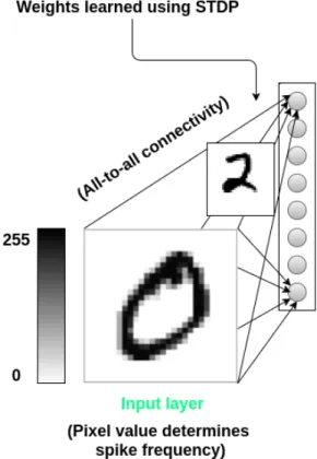
The SNN model presented here is a two-layer feedforward network consisted of 784 neurons in the input layer (equal to the size of an MNIST image which is 28×28), and eight inhibitory neurons in output layer for classifying six different input patterns. Each neuron in the input layer connected to all the neurons in the output layer through a weighted synaptic connection (See Figure 3.1 ). Input neurons in the first layer require spike trains, and we should encode the input image to a train of spikes in which the frequency of the spike pattern is proportional to the intensity of the pixel in the input image. The membrane potential of the neuron updated after each time step according to the learning rule and the associated synaptic weights. First firing output neuron inhibits all the other neuron in the output layer form generating spikes and win the competition for the specific input pattern.

(64)

Figure 3.1: Proposed SNN architecture for image classification.

3.2.1

MNIST dataset

The MNIST database [29] (which stands for Modified National Institute of Standards and Technology database) is a big database of gray scale handwritten digits which widely adopted for training of various image processing methods.

(65)

Figure 3.2: Sample images from MNIST test set.

The database contains 60,000 training and 10,000 testing images, each of the size 28×28 pixels. The intensity of each pixel in the image represented by a number in range 0 to 255 in which higher numbers correspond to bright colors and darker shades represented by small values. Figure 3.2 illustrates sample images of the MNIST test set.

3.2.2

Input Encoding

Input images to the network are six arbitrary images of the MNIST dataset illustrated in Figure 3.3. Each image is of size 28×28 pixels and represented as a matrix in

(66)

which the value of each position is proportionate to the intensity of the corresponding pixel in the input image.

Figure 3.3: Sample images used for classification.

Since this input representation is not understandable for our spiking neural network, we should encode the image input to train of spikes in which the frequency of the spike train is proportional to the intensity of the pixel in the image. This type of encoding in which the information represented as the firing rate of the neuron called rate coding.

3.2.3

Neuron Model

Considering a spike response model (SRM), the postsynaptic neuron generates a potential (postsynaptic potential) whenever it receives a presynaptic spike. This potential is excitatory whenever the membrane potential increased and is inhibitory when it decreased. To determine the instant value of membrane potential, we need to aggregate all existing PSP at the neuron input. When the membrane potential exceeds the critical threshold value, neuron generates an action potential and enter its refractory period. During the refractory period, neuron is overpolarised and is not able to generate action potentials. After this short period, membrane potential resets to its resting value and can produce spikes again. Input neurons in the first layer require spike trains, and we should encode the input image to a train of spikes in which the frequency of the spike pattern is proportional to the intensity of the pixel

(67)

in the input image.

We can describe the postsynaptic function as follow:

PSP(t) =e(−τmt )−e(− t

τs) (3.1)

Where τm and τs are the time constants that describe the steepness of the curve for LTP, and LTD respectively, andtis the time after the arrival of the presynaptic spike. Denoting the threshold value by υ, we can present the refractory ηfunction by equa-tion

η(t) = −υe(τrt )H(t) (3.2)

HereH is the Heaviside function, andτris the time constant for the refractory period. Considering a train of spikes Fi =

n

t(_ig), ... , t(_iK)o arriving at a postsynaptic neuron, we can write the potential equation for j-th neuron as (Eqn.3.3)

Pj = K X i X t(_ig)∈Fi wijPSP(∆tij) X t(_jf)∈Fj ηt−t(_jf) (3.3)

Where ∆tij is the time difference between presynaptic spike and the change in post-synaptic potential considering the delay dij, and described by equation

∆tij =t−t

(g)

i −dij (3.4)

(68)

Simplified SRM Neuron [22]

Without losing the generality of the SRM model, we can consider a simplified model of spike response model as [22] in which the membrane potential of the postsynaptic neuron increases according to incoming spike trains Sit, i = [1, ..., n]. On the other hand, the membrane potential decreases by a constant value D in every time instant (considering time instants as discrete values).

The postsynaptic potential donated by (Eqn.3.5)

Pt=                Pt−1+ n X i=1 WiSit−D, ifPmin < Pt−1 < Pthreshold Prefract ifPt−1 ≥Pthreshold PR ifPt−1 ≤Pmin <0 (3.5)

Figure 3.4 illustrates the membrane potential of the simplified neuron in response to random input spike trains for a duration of 50 time units.

(69)

Figure 3.4: Membrane potential of the simplified neuron in response to random input spike train.

3.2.4

Learning Rule

A pair-based spike time-dependent plasticity rule employed to update synaptic weight connections. Generally speaking, we can explain the STDP rule as follow:

• All the synaptic connections which contribute in the firing of the postsynaptic neuron should strengthen, and in other words, we should increase their associ-ated weights.

(70)

should weaken, and the learning rule reduces their corresponding weights.

Here, the firing rate of the presynaptic neurons is proportional to the intensity of the input signals. The frequency of the spike train transferred to the postsynaptic neuron depends on the strength of the synaptic connection. Whenever the membrane potential of the postsynaptic neuron exceeds the threshold value, it generates an action potential. At this moment we should monitor all the presynaptic neuron which have produced spikes immediately before the postsynaptic neuron, and increase their corresponding synaptic weights.

The weight change in the synaptic connection represented in equation (Eqn.3.6). Note that this change is inversely proportional to the time difference between pre and postsynaptic firing. See Figure 3.5.

STDP(∆t) =      A+e−∆t/τ+ if ∆t >0 A−e∆t/τ− if ∆t <0 (3.6)

(71)

Figure 3.5: STDP curve of (Eqn.3.6).

Here,A+andA−are respectively positive and negative constant of the weight change. τ+ _and _τ− _{are time course of the LTP and LTD, which describe the steepness of the}

function.

The total weight change ∆w presented as:

∆w= N X f=1 N X n=1 STDP(tn_i −tf_j