Augmented UAS navigation in GPS denied terrain environments using synthetic vision

(1)

2016

Augmented UAS navigation in GPS denied terrain

environments using synthetic vision

Teng Wang

Iowa State University

Follow this and additional works at:

https://lib.dr.iastate.edu/etd

Part of the

Robotics Commons

This Dissertation is brought to you for free and open access by the Iowa State University Capstones, Theses and Dissertations at Iowa State University Digital Repository. It has been accepted for inclusion in Graduate Theses and Dissertations by an authorized administrator of Iowa State University Digital Repository. For more information, please [email protected].

Recommended Citation

Wang, Teng, "Augmented UAS navigation in GPS denied terrain environments using synthetic vision" (2016).Graduate Theses and Dissertations. 15835.

(2)

vision

by

Teng Wang

A dissertation submitted to the graduate faculty in partial fulfillment of the requirements for the degree of

DOCTOR OF PHILOSOPHY

Major: Computer Engineering

Program of Study Committee: Arun K. Somani, Major Professor

Joseph Zambreno Nicola Elia Namrata Vaswani

Peter Sherman

Iowa State University Ames, Iowa

2016

(3)

TABLE OF CONTENTS

LIST OF TABLES . . . v

LIST OF FIGURES . . . vi

ACKNOWLEDGEMENTS . . . x

ABSTRACT . . . xi

CHAPTER 1. GPS DENIED UAS NAVIGATION . . . 1

1.1 Problem . . . 1

1.2 Overview of Literatures on Vision Based UAS Navigation . . . 3

1.2.1 Related Work: Landmark Based Approach . . . 3

1.2.2 Different Approaches . . . 4

1.3 Motivation . . . 6

1.4 Research Contributions . . . 7

1.5 Thesis Organization . . . 9

CHAPTER 2. REAL-TIME TERRAIN GENERATION . . . 10

2.1 MetaMap . . . 10

2.1.1 Map Source Selection . . . 10

2.1.2 GRRR Organization . . . 11

2.1.3 DEM Interpolation . . . 14

2.2 GPU Render . . . 16

2.2.1 Pixel Displacement Mapping . . . 16

2.2.2 Ray Surface Intercepting . . . 18

2.3 Experiment . . . 22

(4)

CHAPTER 3. NATURE’S SIGNATURE . . . 25

3.1 Definition Of Minutiae . . . 26

3.2 Drainage Pattern Extraction . . . 27

3.2.1 Diffusion Filtering . . . 27 3.2.2 MLSEC Operator . . . 29 3.3 Minutiae Extraction . . . 30 3.3.1 X-Y Coordinate . . . 31 3.3.2 Orientation . . . 31 3.4 Experiments . . . 33

3.4.1 MLSEC-based Drainage Pattern Extraction . . . 33

3.4.2 Minutiae Extraction . . . 36

3.5 Conclusions . . . 37

CHAPTER 4. MINUTIAE BASED LOCATING IN TERRAIN . . . 38

4.1 Shape Context Descriptor . . . 40

4.1.1 Minutiae Shape Descriptor . . . 40

4.1.2 Crease Shape Descriptor . . . 42

4.2 Registration . . . 43

4.2.1 Affine Transform . . . 44

4.2.2 Reference Minutiae Pair Selection . . . 45

4.2.3 Terrain Similarity . . . 48

4.3 Experiments . . . 48

4.3.1 Experiment 1 . . . 49

4.3.2 Experiment 2 . . . 51

CHAPTER 5. GRANULARITY OF DRAINAGE PATTERNS . . . 59

5.1 10m Resolution . . . 59

5.1.1 Hualapai Peak . . . 59

(5)

5.2 5m Resolution . . . 67 5.2.1 Hualapai Peak . . . 67 5.2.2 Kings Peak . . . 71 5.3 2.5m Resolution . . . 76 5.3.1 Hualapai Peak . . . 76 5.3.2 Kings Peak . . . 83 5.4 Conclusions . . . 89

CHAPTER 6. CONCLUSIONS AND FUTURE WORK . . . 93

6.1.1 Minutiae Feature . . . 93

6.1.2 Minutiae-based Terrain Matching . . . 93

6.1.3 Landmark Generation . . . 94

6.2 Future Work . . . 94

(6)

LIST OF TABLES

Table 3.1 Parameter values for terrain valley extraction . . . 34

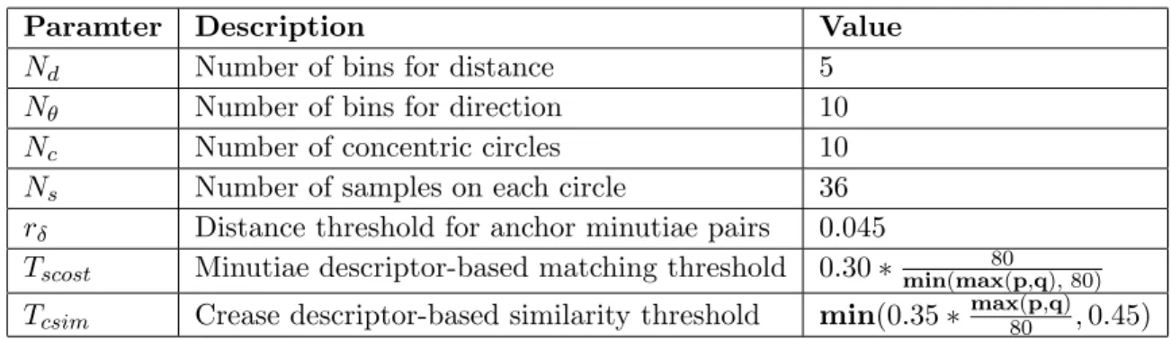
Table 4.1 Parameter values for identifying minutiae pairings . . . 49

Table 4.2 Distribution of similarity scores from PVA matches . . . 56

Table 4.3 Distribution of similarity scores from Non-PVA matches . . . 57

Table 5.1 Match results over Hualapai Peak at 10m resolution . . . 63

Table 5.2 Match results over Kings Peak at 10m resolution . . . 66

Table 5.5 Match results over Hualapai Peak at 5m resolution . . . 71

Table 5.8 Match results over Kings Peak at 5m resolution . . . 75

Table 5.11 Match results over Hualapai Peak at 2.5m Resolution . . . 80

Table 5.14 Match results over Kings Peak at 2.5m Resolution . . . 87

(7)

LIST OF FIGURES

Figure 1.1 Layer-based GIS, with each layer representing one common feature.

While not all layers are useful, a good number of them are, includ-ing Structure, Hydrography, Transportation and Elevation layers. In

our system, we only consider the single elevation layer from USGS. . . 2

Figure 1.2 Functional diagram of our map-aided UAS navigation system . . . 7

Figure 2.1 GRRR of tile N40W111 in ESRI ASCII raster format. . . 13

Figure 2.2 DEM of Kings Peak area in Utah. The DEM data in Fig. 2.2a can be found at http://nationalmap.gov/elevation.html . . . 13

Figure 2.3 Basic idea of displacement mapping. This figure can be found in [51]. . 17

Figure 2.4 Basic idea of displacement mapping on fragment shader. . . 19

Figure 2.5 Ray tracing of the height field. . . 19

Figure 2.6 Sphere tracing of view ray with displaced surface. . . 20

Figure 2.7 Aerial Image of Hualapai Peak in Arizona. . . 22

Figure 2.8 GeoTIFF data of Hualapai Peak before preprocessing. The DEM data can be found at http://nationalmap.gov/elevation.html. . . 23

Figure 2.9 Output of GPU Render. . . 23

Figure 3.1 Minutiae Examples, including Crease Ending, Bifurcation, Dot, Island, Enclosure, Spur, Bridge, Trifurcation, and Crossing. . . 27

Figure 3.2 8-adjacency neighborhood ofPij and their unit normal for MLSEC com-putation . . . 29

Figure 3.3 8-adjacency neighborhood ofP for CN computation . . . 30

(8)

Figure 3.5 One example of crease bifurcation, where the orientation valueθis equal

to the angular direction of the crease from the East. . . 31

Figure 3.6 Terrain valley extraction on Hualapai Peak area. . . 35

Figure 3.7 Valley ending and bifurcation extraction on Hualapai Peak area . . . . 36

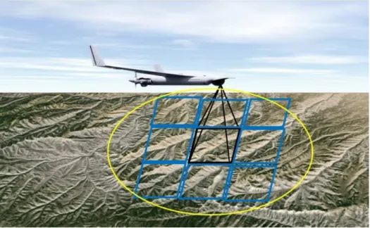
Figure 4.1 The terrain environment shows Kings Peak in Utah. Yellow circle, black rectangle and blue rectangles represents active flight region, aerial image and terrain landmarks, respectively. . . 39

Figure 4.2 Histogram bins used to create minutiae shape descriptor for a given minutiae point. Crease bifurcations and endings are denoted by ‘+’ and ’o’, respectively. . . 41

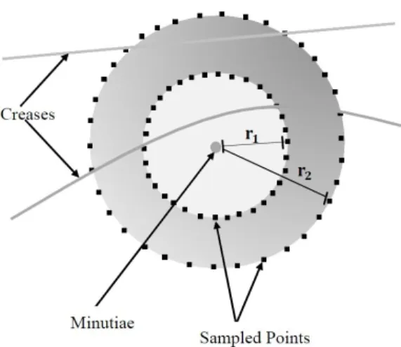
Figure 4.3 Concentric circles to construct local crease shape descriptor of a given minutiae. . . 43

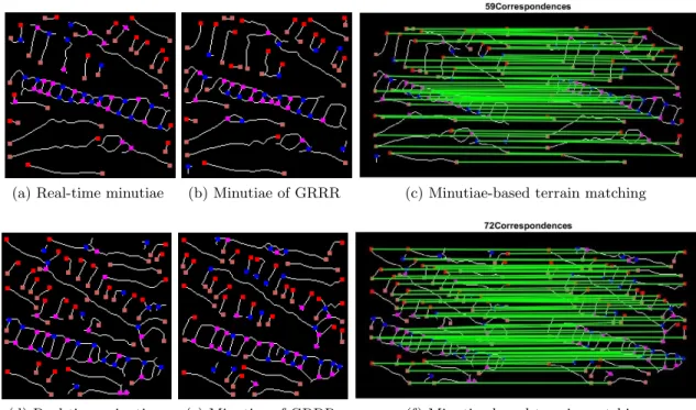
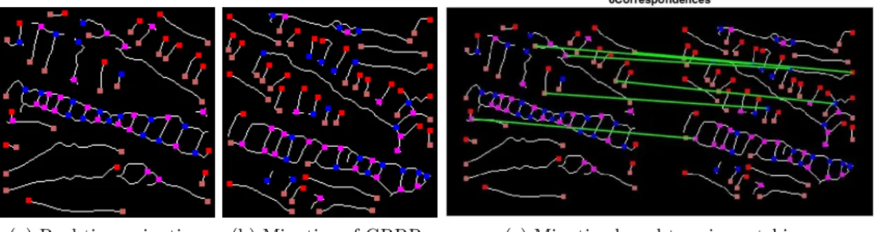
Figure 4.4 Two examples of PVA match over Hualapai Peak area . . . 50

Figure 4.5 An example of Non-PVA match over Hualapai Peak area . . . 51

Figure 4.6 Appearance of one mission section over Ridge Valley Mountain. . . 52

Figure 4.7 Numbers of minutiae in 85 terrain samples over Ridge Valley Mountain. 53 Figure 4.8 Matching results between different terrain blocks over Ridge Valley Mountain . . . 53

Figure 4.9 Appearance of one mission section over Hualapai peak. . . 54

Figure 4.10 Numbers of minutiae in 80 terrain blocks over Hualapai Peak. . . 55

Figure 4.11 Matching results between sample terrains over Hualapai Peak in Arizona 55 Figure 4.12 Frequency histogram of similarity score from PVA matches. . . 56

Figure 4.13 Frequency histogram of similarity score from Non-PVA matches. . . . 57

Figure 5.1 Image data of Hualapai Peak at 10m resolution . . . 60

Figure 5.2 Terrain valleys of Hualapai Peak at 10m resolution . . . 60

Figure 5.3 Numbers of minutiae in nine terrain blocks. . . 61

Figure 5.4 Similarity scores between nine input terrain blocks. . . 62

(9)

Figure 5.6 Frequency histogram of Non-PVA similarity score . . . 63

Figure 5.7 Image data of Kings Peak at 10m resolution . . . 64

Figure 5.8 Terrain valleys of Kings Peak at 10m resolution . . . 64

Figure 5.9 Numbers of minutiae in nine terrain blocks. . . 65

Figure 5.10 Similarity scores between nine terrain blocks. . . 65

Figure 5.11 Frequency histogram of PVA similarity score . . . 66

Figure 5.13 Terrain valleys of Hualapai Peak at 5m resolution. Sizes of both valley images are equal to 1024 by 1024 pixels. . . 68

Figure 5.14 Minutiae numbers in 36 terrain blocks. . . 69

Figure 5.15 Similarity scores between 36 input terrain blocks. . . 69

Figure 5.17 Frequency histogram of Non-PVA similariy score . . . 71

Figure 5.18 Terrain valleys of Kings Peak at 5m resolution. Sizes of both crease images are equal to 1024 by 1024 pixels. . . 72

Figure 5.20 Similarity scores between 36 terrain blocks. . . 73

Figure 5.22 Two terrain blocks missed by our terrain matching algorithm. . . 74

Figure 5.24 This figure shows terrain valleys of Hualapai Peak at 2.5m resolution. Sizes of both valley images are equal to 2048 by 2048 pixels. . . 77

Figure 5.29 25 terrain blocks missed by our terrain recognition approach . . . 81

Figure 5.30 An example of terrain miss . . . 82

(10)

Figure 5.32 Terrain valleys of Kings Peak at 2.5m resolution. Size of both valley

image is equal to 2048 by 2048 pixels. . . 84

Figure 5.37 15 Terrain blocks missed by our terrain recognition approach . . . 88

Figure 5.38 An example of terrain miss . . . 89

(11)

ACKNOWLEDGEMENTS

I would like to take this opportunity to express my thanks to those who helped me with various aspects of conducting research and the writing of this thesis. First and foremost, Dr. Arun K. Somani for his guidance, patience and support throughout this research and the writing of this thesis. His insights and words of encouragement have often inspired me and renewed my hopes for completing my graduate education. I would also like to thank my committee members for their efforts and contributions to this work: Dr.Joseph Zambreno, Dr.Nicola Elia, Dr.Namrata Vaswani and Dr.Peter Sherman. I would additionally like to thank my parents for their supports throughout my whole graduate career.

(12)

ABSTRACT

GPS is a critical sensor for Unmanned Aircraft Systems (UASs) navigation due to its accu-racy, global coverage, and small hardware footprint. However, GPS is subject to interruption or denial due to signal blockage or RF interference. In such a case, position, velocity and altitude (PVA) performance from other inertial and air data sensor is not sufficient for UAS platforms to continue their primary missions, especially for small UASs.

Recently, image-based navigation has been developed to address GPS outages for UASs, since most of these platforms already include a camera as standard equipage. This thesis develops a novel, automated UAS navigation augmentation scheme, which utilizes publicly available open source geo-referenced vector map data, in conjunction with real-time optical imagery from on-board monocular camera to augment UAS navigation in GPS denied terrain environments. The main idea is to analyze and use terrain drainage patterns for GPS-denied navigation of small UASs, such as ScanEagle, utilizing a down-looking fixed monocular imager. We leverage the analogy between terrain drainage patterns and human fingerprints, to match local drainage patterns to GPU (Graphics Processing Unit) rendered parallax occlusion maps of geo-registered radar returns (GRRR). The matching occurs in real-time. GRRR is assumed to be loaded on-board the aircraft pre-mission, so as not to require a scanning aperture radar during the mission. Once a successful match is made, using a known lens model a final PVA solution can be obtained from the extrinsic matrix of the camera [1]. Our approach allows extension of UAS missions to GPS denied terrain areas, with no assumption of human-made geographic objects.

We study the influence of granularity of terrain drainage patterns on performance of our minutiae-based terrain matching approach. Based on experimental observations, we conclude that our approach delivers a satisfactory performance. We identify the conditions to achieve the desired performance for the input images based on UAS flight altitudes.

(13)

CHAPTER 1. GPS DENIED UAS NAVIGATION

1.1 Problem

An Unmanned Aircraft System (UAS), such as drone, is defined as an aircraft without on-board human pilot. Over the past decade, proliferation of small UASs for militiary uses has led to rapid technological advancement. This advancement provides UAS tremendous potential to create new applications in various research areas. These applications range from scientific data collection [2, 3, 5, 4], to provision of military reconnaissance and intelligence gathering as described in [6, 7, 8, 9, 10, 11].

Accurate position information is an important prerequisite for the effective use of UASs. These UAS platforms require accurate and reliable positioning data for guidance and situa-tional awareness. Today various sensor data are utilized to compute the PVA state of UASs, including inertial sensor, barometric altimeter, 3D magnetic sensor and more [12]. GPS (Global Positioning System) is typically the primary source of reliable position information due to its accuracy, global coverage, and small hardware footprint [13, 14]. However, GPS is subject to interruption or denial due to signal blockage or RF interference, such as through canyons or under forest canopy. When GPS is not available, PVA performance from other inertial and air data sensors is no longer sufficient. These sensor equipages integrate the PVA state over time, which results in cumulative measurement error. This degraded position performance is typically not precise enough for UAS platforms to continue their primary missions, especially for small UASs. These small UAS platforms are typically not equipped with high-end naviga-tion components which would provide higher GPS availability as well as better dead-reckoning performance in the absence of GPS.

(14)

navigation, fusing in all available real-time navigation data, such as radar altimeters, passive imaging sensors, and digital elevation map. Recently image-based navigation algorithms have been proposed to address GPS outage for UASs [17, 18, 20, 21, 22, 23], given that most of UAS platforms already include a camera as standard equipage. Performing navigation with real-time aerial images requires georeferenced data, either images or landmarks as a reference. Georeferenced imagery is readily available, but requires a large amount of storage. A collec-tions of discrete landmarks instead are compact, but must be generated by preprocessing. An alternative, compact source of georeferenced data having large coverage area, is open source vector maps, from which meta-objects can be extracted for matching against real-time cam-era acquired images. For terrain environment, we present a novel, automated UAS navigation scheme, which utilizes publicly available open source geo-referenced vector map data, such as U. S. Geological Survey (USGS), in conjunction with real-time optical imagery from an on-board monocular camera to augment UAS navigtaion in GPS-denied environments.

A Geographic Information System (GIS) is a computerized database management system, which captures, stores, manipulates, analyzes, manages, and presents all types of geographical data [15]. GIS is layer based, with each layer representing one common feature, as shown in

Fig.1.1. For example one layer is for buildings, another for roads, and so on. In our research,

we mainly focus on the terrain layer of GIS. That is to say, we work on UAS navigation augmentation in GPS denied terrain environments.

Figure 1.1: Layer-based GIS, with each layer representing one common feature. While not all layers are useful, a good number of them are, including Structure, Hydrography, Transportation and Elevation layers. In our system, we only consider the single elevation layer from USGS.

(15)

1.2 Overview of Literatures on Vision Based UAS Navigation

Recently different vision-based navigation algorithms have been developed to address GPS outage for UASs. Since most of UAS platforms already include a camera as standard equipage, vision-based navigation does not require much additional hardware or payload. It is worth men-tioning that although video cameras can also be “put out” by some adverse weather conditions, such as heavy cloud cover, vision-based navigation is still an attractive supplement to GPS due to the advantages described above. In practice one challenge of vision-based navigation is how to control error accumulation during flight.

1.2.1 Related Work: Landmark Based Approach

A landmark based navigation approach is proposed in [20]. In this approach, each successive image pair is utilized to reconstruct a 3D terrain map through stereoscopic analysis. The position of the aircraft is estimated by matching this reconstructed terrain map to a pre-stored, 3D digital elevation map (DEM). This approach is a two-dimensional extension of the DTS approach as described in [19].

A more recent work is presnted in [21]. It explores practical implementation as well as sys-tem integration issues. In this approach, the syssys-tem is divided into two parts: relative position and absolute position estimation. Relative position estimation extracts relative displacement from two successive aerial images and computes the current position of the aircraft by accumu-lating relative displacement estimates. The position error from relative position estimation is compensated by absolute position estimation. The absolute position estimation is achieved by the following two approaches: (1) matching aerial image directly to reference images when the aerial image contains distinct geometric structures such as roads and large buildings; and (2) matching recovered elevation map (REM) with pstored DEM information in mountain re-gions without artificial structures. Since reconstruction and matching are performed each time that a position estimate is updated, the approaches in [20] and [21] keep correcting position error during flight. However, since stereopsis is often a difficult inverse problem, the terrain reconstruction process itself is potentially error-prone. This can cause position estimation error.

(16)

Recently, some novel image-based navigation algorithms have been developed. These ap-proaches match real-time camera images to template landmarks, instead of DEM information, in storage to achieve precise navigation. For example, Michaelsen et. al [22, 23] developed a testbed to utilize known constructive features and patterns of salient man-made objects from handbook on infrastructure construction or thesauri. The declarative knowledge is presented as production system, and after the instances of most primitive object types are extracted from aerial image, the hypothesis driven parser is used to control the search.

Celik et. al [17] developed a system called “Meta Image Navigation Augmenters (MINA)”, which utilizes real-time camera images in conjunction with open source map data to aug-ment UAS navigation. MINA considered the transportation layer of GIS from OSM (Open-StreetMap). In this system, visual significance of objects, with precise position in 3D world coordinate system, are analyzed. Only visually distinguishing objects are rendered for naviga-tion augmentanaviga-tion purpose. The features of visually distinguishing objects are pre-stored in the training sets as landmarks. During a flight in GPS-denied environments, matching approaches that work with geometric shapes and parametric curves including weighted K-nearest neighbor classifier, thin plate spline transform and principal component analysis, are applied to match aerial images against templates in the training sets. The matching result is used to augment UAS navigation. This system is proved to perform well in urban areas. It keeps correcting position error during flight. However, this approach could not be directly extended to terrain areas, as the representation and matching methods for artificial structures cannot be applied to terrain.

1.2.2 Different Approaches

Merhav and Bresler [24, 25] developed two position estimators for UAS navigation. The first estimator obtains the position information of UASs by integrating instantaneous velocity estimates. The instantaneous velocity is estimated using inter-frame displacement of the input image sequence and the airplane’s height readings. The second estimator obtains the position information through an extended Kalman filter (EKF). For the EKF, the airplane’s position and velocity are defined as its states, and the inter-frame displacement measurements are

(17)

considered as observation data. Using a theoretical analysis, Merhav and Bresler show that the first estimator suffers from error accumulation due to integration operations while EKF that locks on to the available terrain information does not. However, Merhav’s and Bresler’s paper does not report performance of both estimators on video data. In addition, the motion model used in EKF is rather simple: only the translation motion (no rotation) is considered.

Lerner et al. [26] propose an approach that uses the DEM directly to generate a constraint between the camera’s pose and ego-motion. This leads to a set of nonlinear equations from which in principle one can obtain UAS’s pose as well as 3D motion. The focus of the paper was on expressions of estimation error measures as well as their Monte Carlo simulations, since these measures are functions of various parameters and are too complex to evaluate analytically. However, this paper did not describes how to solve these nonlinear equations in detail.

In other works [27, 28, 29], researchers adapt the SLAM (simultaneous localization and mapping) technique to vision-based robot navigation. SLAM was developed for a robot to estimate its own position as well as the positions of a set of landmarks. This is achieved by using an EKF, which utilizes range measurements from the robot to the landmarks as the observation data. One problem with SLAM is that vision sensors generally do not provide range information, additional data is therefore required to generate the needed range measurements. For example, the technique in [27, 29] requires man-made ground landmarks with knowns sizes, and the technique in [28] requires some ground landmarks with known 3D coordinates.

However, these techniques are not scalable to large area, because they use EKF and is n2

computationally expensive.

He at. al [30] proposed a hierarchical framework to deal with uncertainty and noises in motion field analysis. In this approach, images are decomposed into structural blocks containing distinctive features and non-structural blocks. Motion estimation is done for each structural block through feature tracking. A reliable value is assigned to each estimated motion vector, and only motion vectors with higher reliability are used for camera motion estimation. One problem with this approach is that it couldn’t be applied to terrain area which might not contain structural objects.

(18)

combines them with visual updates in an EKF framework to provide precise orientation in-formation. The states of EKF consist of the position, velocity, altitude of UAS, gyroscope biases, and magnitude of the gravity vector. Vehicle height and motion, which are estimated by tracking corner features between consecutive frames via stereo process, are considered as observation data of KEF. This approach only uses a loosely-coupled kalman filter framework to include the vision updates, instead of incorporating the feature tracks themselves in the kalman filter framework, causing an estimation error.

Recently, Zhang et. al [32] proposed an approach that uses the terrain DEM directly to estimate the position and orientation of UASs. In this approach the position and orientation estimation is formulated as a tracking problem and solved by using an extended Kalman filter (EKF). For the EFK, the UAS’s position, orientation, velocity and angular velocity are defined as its states, and the small number of visually salient pixels (feature points) from the aerial images are defined as the observation data. The state and observation models of the EKF are established based on an analysis of the imaging geometry of the UAS’s video camera in connection with a DEM of the flight area. One problem with this approach is that one needs to consider complex aircraft model. Typically the dynamics of the helicopter is described using a conventional six-degree-of-freedom rigid body model, and therefore EKF requires high computational overhead for derivations.

1.3 Motivation

Based on the discussion in Section 1.2, we conclude that specific type of vision-based

nav-igation algorithm, which match the aerial image (recovered elevation map) against landmarks (digital elevation map) pre-stored in databases to estimate position of UAS, are attractive as they keep correcting PVA state error during flight.

For terrain matching, one alternative is to match the recovered terrain elevation map against pre-stored digital elevation model information. Another alternative is to store map data in database and generate life-like appearances of terrain dynamically during flight. Aerial images can be matched directly against map data-rendered terrain images via feature extraction and matching processes to estimate position of UAS. The terrain reconstruction process itself is

(19)

potentially error-prone. This is because stereopsis is often a difficult inverse problem, and this can cause position estimation error. We therefore propose a novel approach that utilizes aerial images combined with open source map data to augment UAS navigation in GPS-challenged terrain environments.

1.4 Research Contributions

This work build a fully automated system of machine vision algorithms for map-aided nav-igation of UASs, such as ScanEagle, in GPS challenged terrain environments. The system can be divided into five major parts: (1) Imaging Component, (2) MetaMap Component, (3) Land-mark Render Component, (4) Feature Extraction Component, and (5) Matching component, as shown in Fig.1.2.

Figure 1.2: Functional diagram of our map-aided UAS navigation system

Imaging components acquire real-time image data. Metamap component loads open source map data on-board the aircraft pre-mission, and output map data of landmarks in ROIs (Re-gions of Interests) during GPS denied flight. Landmark Render component collaborates with a metamap to generate landmarks, i.e., life-like appearance of terrain areas with distinguishing features that the aircraft is expected to encounter. These acquired and rendered images are enhanced and filtered to emphasize certain terrain features by Feature Extraction component. Matching component then matches aerial images to landmarks to find a match. Once a

(20)

suc-cessful match is made, with a known lens model a final PVA solution can be obtained from the extrinsic matrix of the camera. To achieve this goal, we make the following contributions:

1. Landmark Render Component

– Choose an appropriate open source map data for terrain recreation.

– Develop a real-time terrain generation technique based on per-pixel displacement

mapping.

2. Feature Extraction Component

– Identify, develop and analyze a novel minutiae feature which are minor details on

drainage patterns, for terrain recognition purpose.

– Design, develop and analyze a series of filters to extract drainage patterns from

terrain images and identify minutiae on them.

3. Matching Component

– Identify two shape descriptors to describe neighborhood similarity between different

minutiae.

– Develop a matching process to identify minutiae pairings using shape descriptors

from two input minutiae sets.

– Define and identify a criterion to measure similarity of two input terrain images

based on number of minutiae pairings.

4. Granularity of Drainage Patterns

– Study the influences of granularity of drainage patterns on performance of

minutiae-based terrain recognition approach.

– Develop a requirement for minimum minutiae number in two input terrain images

(21)

1.5 Thesis Organization

This chapter starts by describing the challenges of UAS navigation in GPS challenged environments. We then discuss current approaches for UAS navigation augmentation in GPS denied environments. The rest of this document is organized as follows.

Chapter 2 discuss the selection of an appropriate map source for terrain rendering, and

presents a real-time terrain generation technique using per-pixel displacement mapping in

de-tail. In Chapter 3, we define a novel minutiae feature for terrain recognition purpose and

design a series of filters to extract drainage patterns as well as identify minutiae from raw

ter-rain images. Following this, Chapter 4 descibes the minutiae-based terrain matching process

to measure similarity between two input terrain blocks. Subsequently, we study the influence of granularity of drainage patterns, i.e., flight heights, on performance of our minutiae-based

terrain recognition approach in Chapter 5. Finally, Chapter 6 covers the concluding remarks

(22)

CHAPTER 2. REAL-TIME TERRAIN GENERATION

In this chapter, we discuss open source map selection, and describe in detail the generation of life-like appearance of terrain from open source map data using advanced 3D computer graphics techniques.

2.1 MetaMap

2.1.1 Map Source Selection

GIS captures, stores, manipulates, analyzes, manages, and presents all types of geographical

data. GIS is layer based, with each layer representing one common feature, as shown in Fig.1.1.

Terrain and bathymetry are such layers. Our UAS navigation system interprets GIS data at terrain layer to render metamaps, which are later used for terrain recognition purpose.

Natural layers of GIS are collected by professionals and come in structured forms, some of which are highly specialized to specific tasks. We considered and experimented with a variety of maps, before deciding to integrate GRRR from an open source map provider USGS into our UAS navigation system. Accelerated by the proliferation of small, affordable, and lightweight electronically scanning radar systems as well as UAS, GRRR imaging is becoming an incredible source for logistics. GRRR can be characterized as structured, heterogeneous, and scientifically collected map data with consistent amounts of completeness and standardization of resolution. GRRR has the following advantages.

• GRRR is open-cource. USGS provide it in GEOTIFF numerical format, where other

providers will rather provide a raster image of the same tile. More details about GEOTIFF format can be found in [33].

(23)

• GRRR data is based on ASCII, which is both a very convenient debugging feature, and resistant to data corruption.

• While GRRR can be used in quadrilateral tiles that is not an obligation. It can be

downloaded at any size, shape, or proportions, and does not have to be complete.

• GRRR does not carry any watermarks, legends, brand logos, and other artifacts to be

forcibly rendered on map.

• GRRR is customizable, and this is the primary reason it can be made to suit the

appli-cation. With other map providers, the map always look like how the provider wants it to look. Rendering, aliasing, coloring, compression, line-styles, and many more parameters are their proprietary style of map and cannot be modified.

• GRRR allows finer control over emphasizing particular features of interest of terrain area.

For example, it can be height thresholded. Water bodies can be individually colored or removed together. Vegetation can be dynamically modeled, There are no limits.

GRRR has the following disadvantges:

• Because GRRR requires advanced technologies to generate, it is most densely available

for continental U.S. In other countries, it is generally available, but the coverage and resolution varies.

• Also for above reason GRRR is only modified when major natural disasters happen, and

the changes are to be considered negligible.

2.1.2 GRRR Organization

GRRR data provided by USGS are collected by Shuttle Radar Topography Mission (SRTM). SRTM is an international research project, which recorded data of the entire land mass of the

earth from 60◦N to 56◦S using interferometric synthetic aperture radar (InSAR). It generates

the most complete high-resolution digital elevation model (DEM) of the earth. More details about SRTM, including an overview of the mission as well as the DEM production, and an evaluation of the DEM accuracy, can be found in [34, 35, 36].

(24)

SRTM data are arranged into individual rasterized tiles. Each tile covers one degree of latitude by one degree of longitude. Sampling space for individual points in both latitude and

longitude can be either 1/3 arcsecond, 1 arcsecond, 3 arcsecond, or 30 arcseconds, which are

referred to as SRTM1/3, SRTM1, SRTM3 and SRTM30, respectively. In our application, we choose SRTM1/3 data for terrain generation within United States due to its high resolution. The higher resolution of GRRR data, the more terrain details can be captured by the map data. It is worth mentioning that SRTM1/3 is also called “10 meter” data due to the fact that one arcsecond at the equator corresponds to roughly 30 meters in horizontal extent.

SRTM1/3 data are sampled at one-third arcsecond in both latitude and longitude. The resolution of the map data is one-third arcsecond (i.e., 10m) and the data is only released over United States. Each file of one-third arcsecond tile contains 10812 rows, and each row consists of 10812 cells. That is to say, the dimension of the one-third arcsecond tile is equal

to 10812×10812. Each cell stores an elevation value generated by averaging all radar returns

which fall within that cell. The “average” operation is introduced to reduce the primary error from synthetic aperature radar data, which is speckle and has the characteristic of random noise. All elevations are measured in meters referenced to the WGS84/EGM96 geoid.

An example of SRTM data at 10m resolution is given in Fig.2.1, which shows part of GRRR

data from tile N39W111 in ESRI ASCII raster format. It starts with header information, which defines properties of the raster. Raster properities include its dimension, cell size, as well as

coordinate of the origin of the raster. Here, nrows and ncols are numbers of cell rows and

columns, respectively; xllcornerand yllcornerrepresent longitude and latitude value of the

south western (i.e., lower left) corner of the tile, respectively; cellsize represents size of each cell in degree. The header information is followed by an array of cell elevation values (e.g., 2740.487, 2740.767 and so on) specified in space-delimited row-major order, with each row separated by a carraige return.

As shown in Fig.2.1, tile N40W111 covers one degree of latitude by one degree of longitude,

stretching from N39W111 to N40W110. It’s difficult to display the whole terrain scene in detail due to its large area. We take Kings Peak within the tile as an example for explanation. To facilitate observation, we generate 24-bit grayscale DEM of Kings Peak using GRRR data from

(25)

Figure 2.1: GRRR of tile N40W111 in ESRI ASCII raster format.

SRTM. The DEM is shown in Fig.2.2a. Size of DEM is equal to 512 by 512 pixels. Each pixel

corresponds to one terrain cell of size 10m by 10m. Here, the value of a pixel represents an elevation, instead of a luminance intensity. In detail, the brighter the gray level of a pixel, the

larger the elevation value of the terrain point corresponding to this pixel. Fig.2.2b shows the

aerial image of the same terrain block from monocular camera. By comparing the DEM with the aerial image, we make the observation that networks of ridges and valleys in the terrain appear clearly on the DEM. That is to say, GRRR data from USGS-SRTM has the capability to accurately capture the ridge-valley features in this terrain area.

(a) Grayscale DEM (b) Aerial image

Figure 2.2: DEM of Kings Peak area in Utah. The DEM data in Fig. 2.2a can be found at

(26)

2.1.3 DEM Interpolation

As described in Section 2.1.2, we decide to intergate USGS-SRTM data at 10m resolution

into our navigation system due to its high resolution. This data works very well for UAS applications operating at altitudes ranging from 8000 to 10000 meters. However, in some ap-plications UASs need to operate at a relatively lower altitude, and therefore DEM data at a finer resolution are required. ArcGIS Spatial Analyst provides many options for interpolating spatial data to higher resolutions, including Inverse Distance Weighted (IDW), Ordinary Krig-ing and Spline. In this section, we give a brief description of these approaches and compare their performances.

Inverse Distance Weighted is one deterministic interpolation approach using a set of values at scattered sampled locations. It is based on the assumption that the elevation value at a terrain point is more influenced by values at nearby sampled locations compared to those at distant locations. IDW computes the interpolated elevation value at an unknown point using a linear-weighted sum of the values at sampled locations within search neighborhood.

Math-ematically, IDW assign the value ˆz(x0) to an unknown point x0 using the following equation:

ˆ z(x0) = Pn i=1w(di)·z(xi) Pn i=1w(di) (2.1)

where xi represents the ith sampled location;z(xi) is the measured elevation value at terrain

point xi; di is the distance betweenxi and x0; w(di) is the weight assigned to pointxi, where

w(·) is a decreasing function. The general form of weight function is w(d) = d−µ, where

exponentµis commonly set as 1 and 2. The use of higher exponent will create a more localized

interpolator by decreaseing weights of sampling points which are far away fromx0. More details

about IDW can be found in [37, 38, 46].

Kriging is another method of interpolation that use regionalized variable theory to determine the weights of known values at sampled locations. More details about mathematical description of Kriging can be found in [39, 40, 41]. There are several different types of Kriging, including Ordinary Kriging, Simple Kriging, Universal Kriging and so on. Among these different types

(27)

requirements. It is based on the assumption that there exist constant mean over the search

neighborhood around the unknown point x0. The unknown elevtaion valueZ(x0) at point x0,

as well as value Z(xi) at sampled location xi, i = 1,2,· · · , n, are all interpreted as random variables. Ordinary Kriging aims to develop a linear estimator ˆZ(x0), taking in the form of

ˆ Z(x0) = n X i=1 λiZ(xi), (2.2)

whereλi is the weight assigned to the elevation value at sampled locationxi. The weightλi is

chosen to ensure that the following estimation error

(x0) =Z(x0)−Zˆ(x0) (2.3)

has zero expected value and minimal variance. In other words, Kriging gives the best linear

unbiased predication of the elevation value Z(x0) at point x0. By solving the optimization

problem, we obtain that

         λ1 .. . λn µ          =          0 γ(x1−x2) · · · γ(x1−xn) 1 .. . ... γ(xn−x1) γ(xn−x2) · · · 0 1 1 1 · · · 1 0          −1_         γ(x1−x0) .. . γ(xn−x0) 1          , (2.4)

where γ(·) is the variogram function, and µ represents the lagrange multiplier. Aftering

ob-taining weightλi, the interpolated elevation value at x0 is given as follows:

ˆ z(x0) = N X i=1 λiz(xi), (2.5)

where z(xi) represents measured elevation (i.e., observations) at sampled location xi. More

details about Ordinary Kriging can be found in [42, 43, 46].

Spline is an interpolation method that aims to fit a smooth curve to a set of measured elevations {z(xi)}, i = 1,· · · , n, using a spline function. The spline makes a compromise be-tween two quite different objectives of curve fitting: (1) Accurate fitting to data at sampled locations (2) Interpolation function to be as smooth as possible. Spline acheives these two goals by developing a curve estimate which minimizes the following criterion

n

X

i=0

(28)

where S(·) is the spline function; Pn

i=0{z(xi)−S(xi)}2 represents the sum of deviation from

measured elevations at sampled locations;I(S) measures roughness of the interpolation curve.

α is the parameter controlling the trade-off between fitting accuracy and smoothness of the

curve. More details about spline interpolation can be found in [44, 45]. With fitting curve

available, the estimated elevation at non-sampling pointx0 is calculated as

ˆ

z(x0) =S(x0) (2.7)

Guarneri et al [46] compared accuracy of these three interpolation methods using DEM data from the Quachita Mountains in central Arkansas. In detail, they employ each method to interpolate the 10m DEM to 5m, 2.5m, and 1m resolutions. For each resolution, they compare the absolute mean differences of three methods using surveyed control point. Experiment results prove that there is slight difference in the accuracy between these interpolation methods. Given the similarity in accuracy, processing time becomes a more important factor in deciding which method to employ in our application. Based on the observation in [46] that IDW is the fastest among these three interpolators, we prefer IDW interpolation to generate finer resolution DEM of terrain when needed.

2.2 GPU Render

Render component uses the GRRR data to build a digital elevation model (DEM) of the terrain, and renders them to realistic model.

2.2.1 Pixel Displacement Mapping

Computers represent 3D objects with polygons. The more polygons, the more details can be represented. This works very well for geometric volumes such as cube where few polygons can be used to represent very large objects. However, when it comes to a whole mountain it takes billions of polygons to represent it in 3D as in much detail as it is seen from the on-board aircraft camera. This is a huge computational burden.

Using graphic processors, however we can use fewer polygons (hundreds) to represent a 3D mountain, where simulation of lighting of bumps and dents is interpolated according to

(29)

natural models. In other words, we take a low resolution terrain model and statistically fill in the detail to convincingly make it look like a much higher resolution image taken from an on-board aircraft camera. We achieve this via displacement mapping. Main idea of displacement mapping is to employ a macrostructure to approximate a 3D terrain, and add gemotric details to the macrostructure surface using a height map. The height map describes the difference between the macrostructure and the true terrain model in the direction of the macrostructure normal vector. In detail, displacement mapping takes sample points and displace them along the local normal of the macrostructure surface, as illustrated in Fig.2.3. The displaced distance is determined by the value stored in the height map at the given point. More discussion on displacement mapping can be found in [47, 48, 49, 51].

Figure 2.3: Basic idea of displacement mapping. This figure can be found in [51].

Displacement mapping can be implemented in both vertex and pixel shader. In case of per-vertex displacment mapping, the sample points for displacement refer to vertices of the original or tessellated mesh. The usual implementation of per-vertex displacement mapping iteratively tessellates a base surface (i.e., macrostructure surface), and pushes vertices out along the normal of the highly tessellated surface as described in [50]. However, there are some problems with vertex displacement methods as discussed in [51], which are described as follows.

• The number of vertices in the tessellated surface can be very high. This contradicts to

the objective of displacement mapping in hardware accelerated environment, which is to reduce the number of vertex while keeping surface details.

• Vertex processing power of a graphics processor is usually smaller than pixel processing.

(30)

• Pixel shaders are better equipped to access textures. Most graphics cards will prevent texture access within a vertex shader because it has a high performance cost.

• As vextex shader always executes once for each vertex in the terrain model, the work in

vertex shader in evenly distrubuted over the entire terrain geometry, even those invisible parts, where it’s not needed. However, the work in pixel shader is concentrated on nearby visible components, where it is needed most.

A minor disadvantages of displacement mapping using pixel shader is as follows.

• It is not possible to alter a pixel’s screen coordinate within the shader. That means

per-pixel displacement mapping cannot be used for arbitrary large displacement. This is not a major issue because displacements are almost always bounded in a terrain model.

Based on the above discussion, we prefer to implement per-pixel displacement mapping in our Render Component. In per-pixel dispalcement mapping, the samples points for displacement refer to the points corresponding to the texel centers.

2.2.2 Ray Surface Intercepting

In implementation of per-pixel displacement mapping, the macrostructure geomtery of a terrain goes through the graphic pipeline. When it arrived at fragement shader, the height map is utilized to add details to the macrostructure surface in order to make it look like the true terrain surface. However, we are not allowed to change geometry of the terrain at fragment shader, and therefore the visibility problem needs to be addressed through a ray-tracing like algorithm. It can be imagined as tracing the view ray into the height field in order to find the point which is really seen by the camera. The texture coordinate of the visible point will be used to fetch color and surface normal vector, which are later used for computing pixel

intensity. Fig.2.4 shows basic idea of per-pixel displacement mapping.

A brief mathematical description of Per-Pixel displacement mapping based on ray tracing is given as follows. More details can be found in [51]. Suppose the current fragement shader get one point of the macrostructure surface, with texture coordinate of the point equal to [u, v].

(31)

Figure 2.4: Basic idea of displacement mapping on fragment shader.

The coordinate of the processed point in tangent space can be expressed as (u, v,0). For this

pixel point, we define a view ray connecting the eye and the processed point (u, v,0). The

direction of this view ray is defined by view vector V~ in tangent space. The fragment shader

program aims to find the point on the height field, which is really seen by the view ray V~.

Considering the fact that the visible point is on the height field, its coordinate in tangent space can be expressed in the form of (u0, v0, h(u0, v0)) for some unknown (u0, v0). And therefore this visible point can be identified by solving the equation

(u0, v0, h(u0, v0)) = (u, v,0) +V t.~ (2.8)

for some parametert. The equation might have several solutions, i.e., several points (u0, v0, h(u0, v0)) on the height field which are projected onto the same pixel. But only the intersection closest

to the eye, which is called “first intersection” is of interest. Fig. 2.5 shows an example where

there exist three intersections of the view ray with the height field.

(32)

In our work, we employ the Sphere Tracing technique as described in [52] to find the visible point. This approach is attractive as it solved the aliasing problem caused by the commonly used approach of “Uniform Sampling”. Sphere Tracing uses a distance map and an iterative algorithm to guarantee that the first hit will always be found. To construct a distance map, we define a distance functiondist(p, S) =min{d(p, q), q∈S}for any pointpin texture space,

where S represents a displaced terrain surface. dist(p, S) stores the shortest distance from p

to the closest point on the surfaceS. The distance map for a surfaceS is then defined as a 3D

texture that stores the value of dist(p, S) for each point p. More details about the algorithm

of distance map computing can be found in [53].

Figure 2.6: Sphere tracing of view ray with displaced surface.

This distance map gives a measure of the distance between points in texture space and the displaced surface. This distance map provides all the information to intersect a viewing ray with

the displaced surfaceS. Suppose we have a ray with originp0 and normalized viewing direction

vectord~. Using distance information dist(p0, S), we define a new pointp1 =p0+ dist(p0, S)×d~.

One important property of the point p1 is that it will be outside the surface if its previous

point p0 is outside the surface. We repeat the same operation to define another new point

p2 =p1+ dist(p1, S)×d~, and so on. We make the observation that each point pi+1 is a little

bit closer to the surface compared to the previous point pi, as shown in Fig.2.6. That means,

we could always find the first intersection of the ray with the surface (i.e., visible point) by taking enough samples. More discussion about Sphere Tracing can be found in [52]. Once we obtain the texture coordinates of the intersection point, we compute normal-mapped lighting in tangent space.

(33)

Based on the above discussion, the whole terrain generation procedure based on per-pixel displacement mapping can be summarized as follows:

• Approximate the shape of terrain surface using triangles or quads.

• Generate heightmap of the terrain in raster format using GRRR data from USGS-SRTM.

• Compute tangent-space surface normals using the heightmap and store them in a texture.

• Compute 3D distance map using the heightmap and store it directly in a texture.

• Create a vegetation texture based on terrain elevations, and store it directly in a texture.

• Vertex Shader Program:

1. Project vertex position into screen space and pass through the texture coordinate. 2. Transform the eye vector into tangent space. The tangent-space eye vector is later

used in the fragment shader as the direction of the ray to be traced.

3. Transform the light vector into tangent space. The light vector is later used in the fragment shader for tangent-space normal mapping.

• Pixel Shader Program:

1. March the view ray iteratively by querying the distance map to obtain a consec-utive estimate of the distance and moving along the ray until reaching the closest intersection.

2. Compute normal-mapped lighting by multiplying unit light vector with remapped normal vector at intersection point.

More details about Per-Pixel displacement mapping on GPU as well as its shader implemen-tation can be found in [52].

(34)

2.3 Experiment

We utilize an NVIDIA Quadro 5100 graphics processor to achieve the rendering process. We pick Quadro instead of Geforce GTX 480M for terrain generation due to the fact that Quadro is specifically meant for scientific computing and it offers ECC RAM with FP64 IEEE 754. It is optimized for stability and performance in professional applications, like medicine. The CUDA cores can be accessed readily and it uses a Fermi architecture designed to offer higher levels of performance in CPU calculations.

We experiment the terrain generation approach based on displacement mapping over

Huala-pai Peak (35◦0305900N,113◦4505800W) area in Arizona. Image data of Hualapai Peak from

on-board monocular camera is presented in Fig. 2.7. Size of the aerial image is 512 by 512

pixels, where each pixel corresponds to one terrain cell of size 10m×10m.

Figure 2.7: Aerial Image of Hualapai Peak in Arizona.

We start the rendering process with building the DEM of the terrain, directly utilizing

USGS-SRTM data at 10m resolution. 24-bit grayscale DEM of Hualapai Peak is presented

in Fig.2.8, where pixel intensity value is proportional to terrain elevation. The scenery uses a

virtual camera fixed at zenith, and changes the terrain attitude to reflect aircraft orientation. We employ directional light model to simulate sunlight. Sun position is put in direction of

(0.5,1.0,1.0) based on the time information from UAS inertial sensor. We then compute 3D

(35)

tracing to render the terrain. Output of GPU render is displayed at Fig. 2.9. By comparing

Fig. 2.9 with Fig. 2.7, we make the observation that the rendering process has the capability

to accurately capture both ridges and valleys features of Hualapai Peak.

Figure 2.8: GeoTIFF data of Hualapai Peak before preprocessing. The DEM data can be found at http://nationalmap.gov/elevation.html.

Figure 2.9: Output of GPU Render.

We further test the terrain rendering approach using displacement mapping over different terrain areas. In all experiments, image resolution is fixed, with each pixel corresponding to one terrain cell of 10m by 10m. Experiment results show that the rendering process can shade every

(36)

2.4 Conclusions

In this chapter, we first discuss the selection of open source map data and decide to choose GRRR data from USGS-SRTM as our map data for terrain generation purpose due to its high resolution and customizability. We then design a terrain rendering approach using displacement mapping. Experiment results show that the terrain generation approach has the capability to accurately capture drainage pattern features of terrains. In addition, the approach can render

(37)

CHAPTER 3. NATURE’S SIGNATURE

A solution to augment UAS navigation in GPS-challenged terrain environments is decidedly a minutiae-based approach due to the way nature behaves. The following principal observations of the features of nature have led to our proposed approach.

1. Acts-of-nature type terrain features, which present themselves as “detectable” to a ma-chine vision system using some generalizable method, are that of those shaped by flow of water. Water leaves a signature that has a random distribution and can be statistically analyzed. This cannot always be precisely predicted. Common denominator in such prob-lems, where heuristic methods are involved in matching, is that exhaustive approaches (e.g., correlation), and are impractical.

2. The positive artifacts of filtering video signals that contain water-shaped terrain using convolution kernels yield results that visually resemble minutiae formations. Spectral filters for example do not have that type of characteristics. For this reason, they would not work well with nature as they do with human-made scenes.

Observation (1) rules out correlation based approaches because the search would have to be a brute force method. Correlation itself is a second polynomial order computation and is expensive. It also would yield too many false negatives. Only under a perfect and most ideal conditions one would find a match. Observation (2) means that a method cannot guarantee optimal solution. This also means that approaches that work with geometric shapes and para-metric curves have to be eliminated. While some parapara-metric curves are found in nature, they are at a micro level and not a macro level. Mountain size objects tend not to exhibit themselves. This eliminates non-minutiae approaches.

(38)

Once we choose a minutiae-based approach, we need two sources of input that can be represented in minutiae format: (A) a processed image (from monocular camera) to be matched; and (B) templates (from GPU render) to match. The solution needs to be a relaxation of the process of finding a satisfactory correspondence matching between the two via cognitive shortcuts. We can use optimized shortcuts and come up with the most likely matching result in a probabilistic manner.

3.1 Definition Of Minutiae

Minutiae are the minor or incidental details of the terrain that are ambiguous on their own. They have spatial characteristics that can be used to uniquely identify a particular geo-location. These details are found in drainage patterns (a.k.a. creases, ridges, valleys) formed by movement of water flows, and captured in the bathymetry layer of GIS system. Note that we are not assuming presence of water; only that it had once been at that location. Some drainage patterns date as far back as the ice age, and the water that shaped that area is long gone. On the other hand, a small creek or river which still has water flow is still perfectly

applicable. A few minutiae type examples are depicted in Fig.3.1 and described below.

a. Crease Ending: A point at which one terrain crease terminates

b. Bifurcation: A point at which one terrain crease divides into two creases

c. Dot: An isolated crease unit whose length approximates its width in size

d. Island: A terrain crease slightly longer than dots, occupying space between two tem-porarily divergent creases

e. Enclosure: A single terrain crease that bifurcates and reunites

f. Spur: A bifurcation point at which one short crease branches off a longer crease g. Bridge: A connecting crease between two parallel running terrain creases h. Trifurcation: A point at which one terrain crease divides into three creases

(39)

i. Crossing: A point at which two terrain creases cross each other

(a) (b) (c) (d) (e)

(f) (g) (h) (i)

Figure 3.1: Minutiae Examples, including Crease Ending, Bifurcation, Dot, Island, Enclosure, Spur, Bridge, Trifurcation, and Crossing.

Pliability of the underlying rock to water, deposition pressure of water, slippage, roughness of the substrate are just some of the various factors that determine how water forms drainage patterns. Drainage patterns govern how minutia are formed such that no two terrains are exactly alike. Our approach is designed to bring out these signature features, while filtering out minor changes in impressions of the same terrain area recorded at different times with different ambient lightning, orientation, or seasonality.

Although minutiae are readily present in most terrain, they are not in an immediately usable form due to the ambient lighting, color, shadows, and many other factors that they are usually hidden within. As minutiae appear as minor details in drainage patterns, we first employ diffusion filtering followed by MLSEC operator, to expose drainage patterns.

3.2 Drainage Pattern Extraction

3.2.1 Diffusion Filtering

Because minutiae appear as minor details in drainage patterns, we first propose a “crease-ness” measure to extract drainage patterns. A pre-filtering step is required to reguralize the raw terrain image in order to obtain stable and meaningful crease result. We employ an anisotropic nonlinear diffusion process as described in [55] to achieve this. The advantages of this filtering process are that while crease features are enhanced, artifacts are not created and junctions are

(40)

not interrupted. A brief discussion of the diffusion filtering based on structure tensor is given as below. The main idea of the diffusion filtering is to construct a coarse creaseness measure, and control the diffusion strength in the presence of ridges and valleys (i.e., enhancing diffusion

along the crease while avoiding smoothing across crease). For that, we consider normalized

Hessian matrix H of a two-dimensional image I such that

H = p 1 1 +k∇Ik2    ∂2_I ∂x2 ∂ 2_I ∂x∂y ∂2_I ∂y∂x ∂2_I ∂y2    (3.1)

where ∇I is image gradient. Then a multilocal representation Hρ of the normalized Hessian

matrixH is constructed by making a double regularization step as follows:

Hρ=Gρ∗    1 p 1 +k∇Iσk2    ∂2_I σ ∂x2 ∂ 2_I σ ∂x∂y ∂2_I σ ∂y∂x ∂2_I σ ∂y2       (3.2)

whereIσ is Gaussian-smoothed version ofI and σis standard derivation of the Gaussian filter;

Gρ is a Gaussian kernel with standard derivation equal toρ for regularizing the tensor field.

By denoting eigenvalues of the multilocal normalized Hessian matrix Hρ as κ1 and κ2, we

define the following two descriptors

µr=      ˜ κ1−˜κ2 ˜ κ1+˜κ2 if κ1 <0 0 if κ1 ≥0 , (3.3) µv =      ˜ κ1−˜κ2 ˜ κ1+˜κ2 if κ1>0 0 if κ1≤0 , (3.4)

where ˜κ1 = max(|κ1|,|κ2|) and ˜κ2 = min(|κ1|,|κ2|), to detect ridges and valleys, respectively.

It’s worth mentioning that µr and µv reach their highest value of 1 in the presence of ridges

and valleys, respectively, as described in [56, 57, 58, 59].

We denotev1 andv2 as the directions corresponding to the greatest and lowest

eigen-value in absolute eigen-value, respectively. v1 andv2 can also be interpreted as the directions across

and along the local crease, respectively. Thediffusion tensorDis constructed to have the same

eigenvectors v1 and v2 as Hessian matrixHρ. The eigenvalues of Dare chosen as

λ1= ∈(0,1)

λ2=αµr+βµv α, β∈[0,1],

(41)

where α and β control the diffusion strength in the local crease direction in the presence of

ridges and valleys, respectively; the value controls the diffusion strength across the crease.

The positive value ofensures the semidefinite property of the diffusion tensor D.

Using creaseness diffusion tensor D, we filter the terrain image through the following

diffu-sion equation.

∂I

∂t = div(D· ∇I) (3.6)

We employ the discrete method (convolution in discrete domain) as described in [60] to solve the continuous diffusion equation.

3.2.2 MLSEC Operator

The creaseness measure we employ for crease extraction is known as a Multilocal Level-Set Extrinsic Curvature (MLSEC) developed in [61]. This is inspired from medical imaging as it is employed in arterial imaging. We have modified this approach to work with drainage patterns because the model of randomness exhibited by human circulatory system is in parallel to that of the drainage patterns in nature. Creases constructed by MLSEC are invariant with respect to spatial translation, spatial rotations, and uniform spatial magnification, and contain

fewer crease discontinuities. Here, we consider the case in 2D (d = 2) with B composed of

the eight nearest neighbors of each pixel (r = 8). That is, for the pixel Pi,j of coordinates

[i, j], we have B={Pi,j−1, Pi+1,j−1, Pi+1,j, Pi+1,j+1, Pi,j+1, Pi−1,j+1, Pi−1,j, Pi−1,j−1} and N =

{nN,nN E,nE,nES,nS,nSW,nW,nW N}as shown in Fig. 3.2.

(42)

3.3 Minutiae Extraction

Although nine types of minutiae are introduced in Section3.1, we primarily focus on crease

endings and bifurcations, which have been proved to be the most distinguishing in [63, 64]. We

employ the Crossing Number (CN) method from [65] to extract crease endings and bifurcations

from the skeleton crease images. For each crease pixelP, this approach scans its 8 neighbors in

anti-clockwise direction as shown in Fig.3.3, and computes the intensity difference in absolute

value between two adjacent neighbors. TheCN value of a crease pixelP is then defined as the

sum of intensity differences divided by 2, as given in the following equation:

CN = 0.5

8

X

n=1

|I(Pn)−I(Pn+1)|, P9 =P1 (3.7)

where I(Pn) represents the intensity value of pixel Pn. Intensity values of a crease and

non-crease pixel in the non-crease image are equal to 0 and 1, respectively.

Figure 3.3: 8-adjacency neighborhood ofP for CN computation

For this formula, if CN = 1, the pixel corresponds to the crease ending, and ifCN = 3, the

pixel corresponds to a bifurcation, as shown in Fig.3.4. In this figure, blue and white squares

represent crease and non-crease pixels, respectively.

(43)

In our research work, we represent a minutiae using quaternary structure. Each minutiae mk is described as mk = {xk, yk, θk, Tk}, where xk and yk represent the normalized x and

y coordinates of the minutiae, respectively; θk represents the angular direction of the crease

associated with the minutiae as shown in Fig. 3.5; andTk refers to the type of minutiae (e.g.,

endings or bifurcations). Once we identify minutiae mk using CN operator, we compute its

coordinatesxk and yk, as well as orientation θk, as described in Section 3.3.1and 3.3.2.

Figure 3.5: One example of crease bifurcation, where the orientation value θ is equal to the

angular direction of the crease from the East.

3.3.1 X-Y Coordinate

Suppose pixel P of coordinate [i, j] on 2D image plane is identified as minutiae mk, then

X-Y coordinate (xk, yk) of minutiae mk is computed as follows:

xk=j/W, (3.8)

yk= (H+ 1−i)/H, (3.9)

whereW andH represent width and height of the raw terrain image, respectively. It’s easy to

make the observation thatxk∈[0,1] andyk ∈[0,1].

3.3.2 Orientation

Taking advantage of analogy between human fingerpints and drainage patterns, we employ the pixel-wise scheme as described in [67] to estimate the local orientation of creases contained

(44)

in the terrain image. This method is attractive as it produces a finer and more accurate estimation of the orientation field compared to other block-wise approach as described in [66]. The steps for calculating the orientation valueθ(i, j) at pixel P = (i, j) are described below.

1. Identify the block of size W ×W centered at pixel (i, j) in the crease image. For each

pixel (u, v) in the block, compute the graidents in both X and Y directions, denoted

as∂x(u.v) and∂y(u, v), respectively. Here, Sobel operators Gx and Gy are employed to compute∂x(u.v) and∂y(u, v), respectively.

Gx=       1 0 −1 2 0 −2 1 0 −1       Gy =       1 2 1 0 0 0 −1 −2 −1       (3.10)

2. Employ least mean square estimation approach to compute the local orientation θe(i, j)

of pixelP using the following equations.

Vx(i, j) = i+W₂ X u=i−W 2 j+W₂ X v=j−W 2 2∂x(u, v)∂y(u, v) (3.11) Vy(i, j) = i+W₂ X u=i−W 2 j+W₂ X v=j−W 2 ∂_x2(u, v)∂2_y(u, v) (3.12) θe(i, j) = 1 2tan −1Vy(i, j) Vx(i, j) (3.13)

3. Smooth the orientation field in a local neighborhood by converting the orientation field

into a continuous vector field. Gaussian smoothing is performed using the following

equation: Φ0_x(i, j) = w_Φ 2 X u=−wΦ 2 w_Φ 2 X v=−wΦ 2 G(u, v)Φx(i−u, j−v), (3.14) Φ0_y(i, j) = w_Φ 2 X u=−wΦ 2 w_Φ 2 X v=−wΦ 2 G(u, v)Φy(i−u, j−v), (3.15) where Φx(i, j) = cos(2θe(i, j)), (3.16)

(45)

Φy(i, j) = sin(2θe(i, j)). (3.17) Here, Gis a Gaussian filter of size wΦ×wΦ; Φx(i, j) and Φy(i, j) represent the x and y components of the orientation field, respectively.

4. The final smoothed orientation value O at pixel P is defined in Eq.3.18.

O(i, j) =1 2tan −1 Φ 0 y(i, j) Φ0_x(i, j) (3.18)

Once orientation field O is computed, orientation θk of minutiae mk, located at rowiand

columnj is defined in Eq 3.19.

θk =O(i, j) (3.19)

3.4 Experiments

We operate MLSEC-based drainage pattern extraction method as well as CN-based minu-tiae extraction approach on both aerial and GPU-rendered terrain image in order to test effec-tiveness of these two approaches.

3.4.1 MLSEC-based Drainage Pattern Extraction

As map-aided UAS navigation involve matching aerial images against terrain landmarks from GPU render. We experiment MLSEC-based crease extraction approach on both aerial and GPU-rendered terrain images to show its effectiveness. For a terrain, ridges and valleys are dual in the sense that valleys of a terrain image are the ridges of the inverted image. In our work, we focus on terrain valleys. Parameter values for diffusion filtering and crease orientation

estimation are given in Table 3.1. It is worth mentioning that values of parameter K,σ and

w1 depend on spatial resolution of terrain images. σ andw1 control the extent of initial image

smoothing in order to obtain robust derivatives. The higher resolution of the terrain image, the

larger values of σ and w1 are to take more neighboring pixel information into consideration.

K control diffusion strength. The larger value of K, the sharper crease features we obtain.

(46)

this scenario, we experimentally set K as 5 based on the observation that further increase in

K could not help improve performance. Besides, we set σ and w1 as 1 and 5, respectively, in

order to smooth the terrain image while keeping minor drainage patterns. Based on discussion in [55], we set ,α and β as 0.001, 1, and 1, respectively for ridge-valley diffusion.

Table 3.1: Parameter values for terrain valley extraction

Paramter Description Relevance Value

K Total iteration number for diffusion filtering Diffusion process 5

σ Standard derivation of Gaussian filter used to smooth original mountain images Diffusion process 1

w1 Size of Gaussian filter used to smooth original mountain images Diffusion process 5

ρ Standard derivation of Gaussian kernel used to regularize the tensor field Diffusion process 1

w2 Size of Gaussian kernel used to regularize the tensor field Diffusion process 3

Parameter controlling the diffusion strength in the direction across the creases Diffusion process 0.001

α Parameter controlling the diffusion strength along creases in presence of ridges Diffusion process 1

β Parameter controlling the diffusion strength along creases in presence of valleys Diffusion process 1

W Block Size Orientation Estimation 16

σs Standard deviation of Gaussian filter used to smooth orientation field Orientation Estimation 3

wΦ Size of Gaussian filter used to smooth orientation field Orientation Estimation 6∗σs= 18

We experiment with MLSEC based crease extraction approach over Hualapai Peak area (35◦0305900N,113◦4505800W) in Arizona to extract terrain valleys. Terrain images of Hualapai

Peak from monocular camera and GPU render are shown in Fig.3.6aand Fig.3.6d, respectively.

Size of both images are equal to 512 by 512 pixels, where each pixel corresponds to one terrain

cell of 10m by 10m. We apply the crease extraction approach on these two images, and

display the extracted terrain valleys from aerial and rendered images in Fig.3.6band Fig.3.6e,

respectively. To facilitate observation, we overlap extracted valleys from both aerial and

GPU-rendered images with the greyscale terrain image, and present the results in Fig. 3.6c and

Fig.3.6f, respectively. In these two figures, black pixels represent extracted terrain valleys. We make the following observations from experimental results: