Optimal Electric-Power Distribution and Load-Sharing on Smart-Grids: Analysis by Artificial Neural Network
Dr. Dolores De Groff, Ms. Roxana Melendez, Dr. Perambur S. Neelakanta, Ms. Hajar Akif College of Engineering and Computer Science, Florida Atlantic University, Boca Raton, Fl. 33431
Email: [email protected], [email protected], [email protected], [email protected] Abstract
This study refers to developing an electric-power distribution system with optimal/suboptimal load-sharing in the complex and expanding metro power-grid infrastructure. That is, the relevant exercise is to indicate a smart forecasting strategy on optimal/suboptimal power-distribution to consumers served by a smart-grid utility. An artificial neural network (ANN) is employed to model the said optimal power-distribution between generating sources and distribution centers. A compatible architecture of the test ANN with ad hoc suites of training/prediction schedules indicated thereof. Pertinent exercises to determine smartly the power supported on each transmission-line between generating to distribution-nodes. Further, a “smart” decision protocol prescribing the constraint that no transmission-line carries in excess of a desired load. An algorithm is developed to implement the prescribed constraint via the test ANN; and, each value of the load shared by each distribution-line (meeting the power-demand of the consumers) is elucidated from the ANN output. The test ANN includes the use of a traditional multilayer architecture with feed-forward and backpropagation techniques; and, a fast convergence algorithm (deduced in terms of eigenvalues of a Hessian matrix associated with the input data) is adopted. Further, a novel method based on information-theoretic heuristics (in Shannon’s sense) is invoked towards model specifications. Lastly, the study results are discussed with exemplified computations using appropriate field data.
Indexing terms/Keywords: Artificial neural network, Backpropagation algorithm, Load-sharing, Smart-grid, Electric-power grid
Subject Classification: Neural Networks
Type (Method/Approach): Computational research Supporting Agencies:
Introduction
In modern contexts metro areas conform to expanding turfs of electric power utility systems. Relevant expansions via-á-vis growing population and geographical size, correspond to exponentially increasing electric-power consumption in service locales; hence, it has become a necessity to analyze the underlying infrastructure towards establishing an optimal power-sharing protocol at the end-nodes serving domestic, commercial and
node, which is an endpoint or distribution connection point for power transmissions on the network that can process or forward the power transmissions to other nodes meeting the demand posed.
The smart-grid represents the full suite of initiatives, protocols and current as well as proposed responses to demand versus supply challenges in electricity utility systems. The smart-grid, in general, makes use of the technology such as state estimation* that would improve fault-detection and allow self-healing of the network (without the intervention of technicians-in-loop). This will also ensure more reliable supply of electricity and reduce the vulnerability to natural disasters and/or man-made attacks. (State estimation*: Fred Schweppe in 1968 defined state estimator as “a data processing algorithm for converting redundant meter readings and other available information into an estimate of the state of an electric power system”).Although, smartly-designed multiple, new routes are required in smart-grids, the „old grid‟ would also coexist in the infrastructure participating in the multiple routes.
Smartly implied next-generation transmission and distribution infrastructure has the flexibility towards handling bi-directional energy flows; and, it allows distributed generation from a variety of sources (such as, from photovoltaic panels on building roofs, fuel cells, wind farms, and other renewable energy sources). Mostly, existing network infrastructure is not built to allow multiple distributed feed-in points; and, typically, even if some feed-in is allowed at the local (distribution) level, the transmission-level infrastructure may not accommodate it. As such, smart-grid technology has become a necessary condition in order to sustain very large amounts of renewable electricity on the grid facing rapid fluctuations in distributed generation caused by cloudy or gusty weather [1].
Based on the broad definition of a smart power-grid as above, this study focuses on developing an optimal/suboptimal electric-power distribution across the complex and expanding metro power-grids. An artificial neural network (ANN) is used for optimal decisions of load-sharing on a smart grid. Relevantly, for the grids to operate economically and reliably, demand-forecasting on the service profile is essential inasmuch as, it could enable predicting the amount of optimal power required to be distributed to consumers. Need for such a demand-forecasting effort has motivated this study.
Hence, a traditional multilayer ANN architecture (based on feed-forward and backpropagation techniques) with a fast convergence algorithm is developed and used for the said demand-forecasting; and, the ANN simulations done include using pseudo-forms of power-line data established via statistical bootstrapping. The results of simulation experiments so obtained illustrate and validate the proposed method.
Optimal Power Distribution
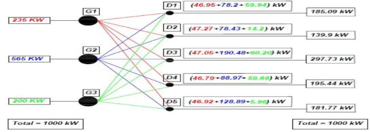
In all, the scope of this study, the problem is to indicate a smart forecasting strategy on optimal/suboptimal power distribution to consumers. Pertinent details are as follows: The proposed method is illustrated in Figure 1 where, the schematic details of an optimal power-distribution system envisaged between generating sources and distribution stations are shown with reference to a hypothetical power distribution scenario.
Figure 1. Schematic of the proposed method of optimal power distribution: Example problem
As illustrated in Figure 1 scenario, there are three power sources designated as generating stations G1, G2, and G3. Assuming a total available power of 1000 kW by the set {G1,G2, and G3} supplying 235 kW, 565 kW, and 200 kW, respectively, it is further considered that there are five distribution centers: D1, D2, D3, D4, and D5 to which the available 1000 kW power has to be “smartly” distributed via transmission-line set {Wij}. That is, there
are fifteen transmission lines interconnecting i = 1, 2 and 3 generating stations with j = 1,2,3,4 and 5 distribution centers.
In order to evolve an optimal/suboptimal electric power-distribution in question, the test ANN being adopted corresponds to a feedforward architecture facilitated with backpropagation of the error. It consists of nine input neuron units, one hidden layer (with nine neuronal units) and one output unit. The supervising teacher value corresponds to the normalized value of the sum of the powers from nine power sources (total available power) of the input set. The test ANN is illustrated in Figure 2.
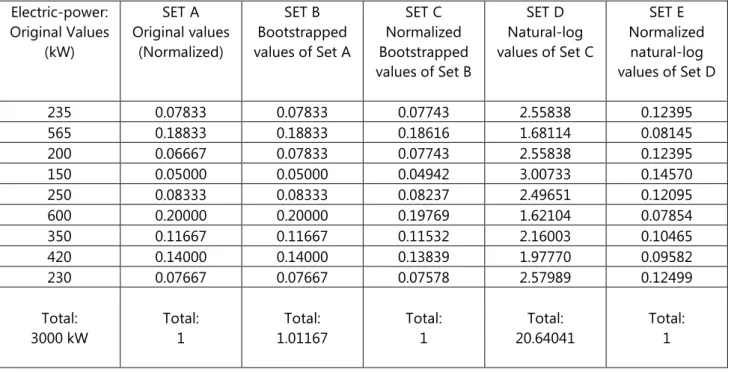
Step I: Suppose the available power generated is given by a set of nine inputs (from each of nine power sources). These data are shown in column 1 (Original values) of Table 1. This original set is then normalized (with respect to the total power generated). This result is shown in column 2 (SET A) of Table 1.
Step II: Using the normalized values as indicated in Step I, construct bootstrapped, pseudoreplicates (of at least twenty) of normalized values from SET A. One example is shown in column 3 (SET B) of Table 1. Results in column 3 are then normalized as shown in column 4 (SET C).
Step III: Obtain natural-log of the constructed normalized pseudoreplicates (SET C above) and take their absolute values. Results are shown in column 5 (SET D). The reason behind this normalization procedure is as follows: The availed ex post input data and prediction phase details should preferably be specified in a demeaned and log-transformed format, so that the underlying log-transformation would allow filtering or data-smoothing of these details; and, this would (partially) minimize the computational burden (due to any outliers). Further, demeaning procedure would allow avoiding the need to specify an intercept term in the estimation of the model. Also the log-formatted data implicitly transforms the details into entropy perspectives (or information-theoretic heuristics in Shannon’s sense [3].
Step IV: Normalize SET D to obtain SET E (column 6). SET E is the input set for the ANN. Twenty such sets are used here for training.
The pseudoreplicates presented in Table 1 denote exemplars of shuffled values of the original set [4]. The cardinality of each pseudoreplicate set is same as the original set; and, for each original set, the number of bootstrapped pseudoreplicates could be as large as 200 [4]. However, it can be limited to 20. That is, the number of pseudoreplicate sets for each original set could be as large as 200 or even higher; however, in this study it is limited to 20 (corresponding to 20 training iterations adopted in the test ANN as described later).
Table 1: Pseudo-forms of Power-line Data Established via Statistical Bootstrapping Electric-power: Original Values (kW) SET A Original values (Normalized) SET B Bootstrapped values of Set A SET C Normalized Bootstrapped values of Set B SET D Natural-log values of Set C SET E Normalized natural-log values of Set D 235 0.07833 0.07833 0.07743 2.55838 0.12395 565 0.18833 0.18833 0.18616 1.68114 0.08145 200 0.06667 0.07833 0.07743 2.55838 0.12395 150 0.05000 0.05000 0.04942 3.00733 0.14570 250 0.08333 0.08333 0.08237 2.49651 0.12095 600 0.20000 0.20000 0.19769 1.62104 0.07854 350 0.11667 0.11667 0.11532 2.16003 0.10465 420 0.14000 0.14000 0.13839 1.97770 0.09582 230 0.07667 0.07667 0.07578 2.57989 0.12499 Total: 3000 kW Total: 1 Total: 1.01167 Total: 1 Total: 20.64041 Total: 1
Backpropagation is effected with the mean-square error () obtained at the output and applied to the weight vector matrix [Wij] as shown in Figure 2 [5]. The values addressed at the input units progressively pass via interconnected inner and hidden layers and provides a summed output, which is squashed by a nonlinear
sigmoid (so to assume a limited level); and, the sigmoid-compressed output is finally compared against a teacher value (representing the desired output prescribed as an objective). The resulting error is sensed and applied to the interconnection weights by a backpropagation gradient algorithm. That is, the sigmoid-compressed value indicates an output, O which is compared against a teacher/supervisory (reference) value, T (representing the desired output objective). The resulting error corresponding to (O − T) expressed in terms of an error-function such asdenoting the mean-squared value of (O − T); and, is then sensed and backpropagated. The
backpropagation (BP) algorithm adopted facilitates typically a steepest descent based gradient that modifies the
set of weight-vector values (either to increase or decrease), when the error-function is applied to the interconnection weights, Wij. The ANN operation as above is as outlined below:
In Figure 2, the summed value (zi) at the output unit corresponds to rth ensemble of inputs {yi}, weighted
across the input-layer (with i = 1, 2, 3 ... I = 9 units) and the hidden-layer (with j = 1, 2, 3 ... J = 9 units). Its linearly-scaled value, K× zi (with K denoting a linear-scaling constant) is subsequently squashed by a hyperbolic tangent (sigmoidal) function, f(.), yielding an output, Oi = f(K× zi). Further, the coefficients of weighting of interconnections between input- and hidden-layers are specified by the set: {Wij}. The topology of the ANN, in
using several ensemble of input-sets, r = 1, 2, 3 ... R. For each ensemble input, the ANN is rendered to a state of convergence via iterative backpropagation of the error. This procedure refers to training or learning phase of the ANN.
Determination of the Learning Rate
As mentioned above, a gradient-based method is employed to adjust the weights proportional to the magnitude of the error, the sign of the error, and the learning rate according to the following equation:
(
)
(
)
(
)
r( )(learning rate)
rw new
w old
w old
sign
(1)
Iterations are repeated towards convergence. The error, r, versus the number of iterations is plotted to get the
learning curve.
De Groff and Neelakanta [6] have shown that the learning rate can be set as inversely proportional to the maximum eigenvalue of the input data set. Convergence depends on the gradient and curvature of the squared error versus the weights. A large eigenvalue would result in a low learning rate and the training would be more reliable. However, it is possible that the result may lead to a smaller eigenvalue and thus a larger learning rate. Such a larger learning rate may result in the training not converging or diverging. Thus, for applications when the learning rate is too large, to avoid divergence; instead, by setting the learning rate = max , it mostly leads
to an optimal solution as indicated in [6].This strategy is implemented in this work.
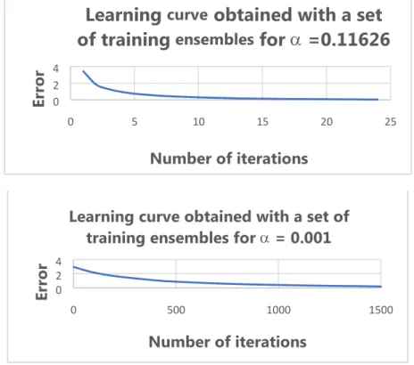
In this study, a comparative assessment of convergence performance of the test ANN is done in terms of number of iterations (towards convergence) ascertained with an arbitrary learning rate (= 0.001)versus the corresponding number of iterations obtained with the learning rate, max. That is, for each of the twenty input
sets, the Hessian eigenvalue is computed; and, the largest of the Hessian eigenvalues, max is chosen and
adopted as the learning rate in training/learning phases. The maximum eigenvalue obtained for the test inputs set ismax = 0.116266 and as such, the learning rate is taken in the simulations as, = 0.116266. (A comparison
of simulated data in terms of relevant learning-curves for an exemplar training ensemble of r = 1 is presented in the later section of Results. )
Prediction Phase of the Test ANN
When all the ensembles of the training (input) set are exhausted, the net is conformed to a final set of
“trained/learned” interconnection weights specified by the matrix, [Wij]tr. That is, the net is now presumably
“trained” and ready to take a fresh set of input data so as provide a (sub) optimal solution or an output comparable to the desired target depicting the objective value, set forth by the supervisory reference. In other words, subsequent to training phase, the test ANN with its trained interconnection weights (specified by the matrix, [Wij]tr) is ready to accept a set of new input values, for which the prediction output is sought. Hence, with
a new input set, the test ANN can be run with the [Wij]tr values; and, using the same teacher value, Ti (adopted
as a supervisory reference in the training phase) under the converged state, the test ANN yields an output (Oi)
value depicting the output being predicted for the new input set addressed. The net operation as above refers to the prediction phase of the test ANN.
In this prediction/testing phase, as stated above, the test ANN is assigned with the converged weight matrix deduced in the training phase[ and, a set of nine inputs is generated randomly using bootstrapping method as discussed earlier. The test inputs are normalized values and [Wij]tr is used to calculate the outputs
of each neuron. For each of the nine test inputs and with the activation function applied to each of the outputs the corresponding summed and squashed value is compared against the teacher objective and the error-value is computed for backpropagation.
Results and Discussion
Developing optimal/suboptimal electric power-distribution and load-sharing across the expanding, complex metro power-grid infrastructure via an ANN-based approach is conceived in this study. The following are pertinent results derived from the simulations performed.
I. Training Phase Results
As said before, the training phase is done with twenty pseudoreplicate sets (of input data) applied to the test ANN. The final weight matrix [Wij]tr obtained at the convergence of the 20th training set is then stored. Relevant
weight matrix corresponds to a fast-convergence performance of the test ANN as described in [6].
As discussed earlier, the learning rate adopted in the aforesaid training schedules refers to = max.
The efficacy of using ( = max) for the learning rate (in lieu of traditional, arbitrarily specified value say, =
0.001) is demonstrated by relevant learning curves deduced. Examples of such comparisons via learning curves obtained for an exemplar training ensemble of r = 1 are presented in Figure 3 considering training phase for forecasting on power distributions smartly across a generating station set {G} and a distribution center set {D}.
Figure 3: Learning curves obtained with the set of training ensembles r =1 using arbitrary learning 0 2 4 0 5 10 15 20 25
Number of iterations
Learning
curve
obtained with a set
of training
ensembles
for
=0.11626
0 2 4
0 500 1000 1500
Number of iterations
Learning curve obtained with a set of
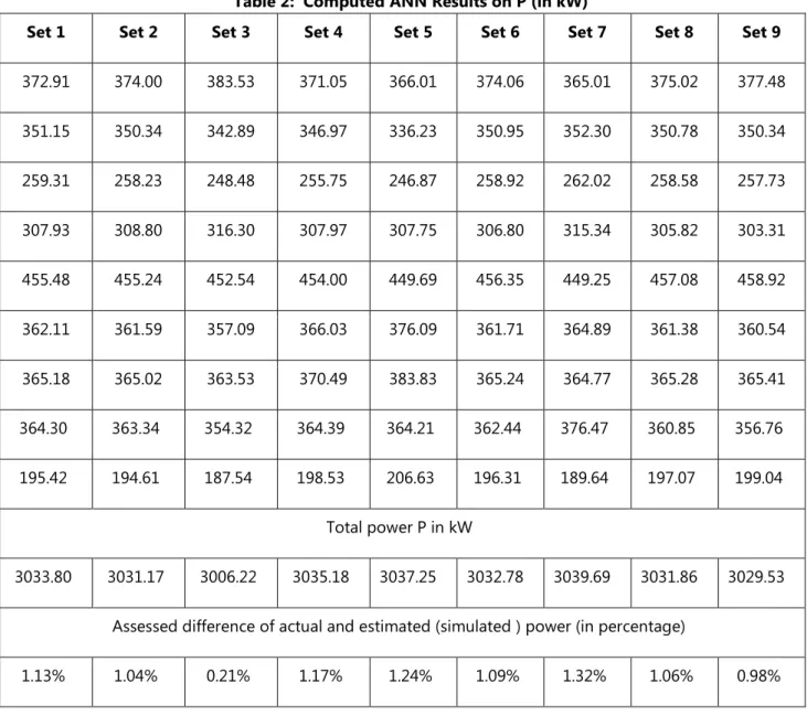
Table 2: Computed ANN Results on P (in kW)
Set 1 Set 2 Set 3 Set 4 Set 5 Set 6 Set 7 Set 8 Set 9 372.91 374.00 383.53 371.05 366.01 374.06 365.01 375.02 377.48 351.15 350.34 342.89 346.97 336.23 350.95 352.30 350.78 350.34 259.31 258.23 248.48 255.75 246.87 258.92 262.02 258.58 257.73 307.93 308.80 316.30 307.97 307.75 306.80 315.34 305.82 303.31 455.48 455.24 452.54 454.00 449.69 456.35 449.25 457.08 458.92 362.11 361.59 357.09 366.03 376.09 361.71 364.89 361.38 360.54 365.18 365.02 363.53 370.49 383.83 365.24 364.77 365.28 365.41 364.30 363.34 354.32 364.39 364.21 362.44 376.47 360.85 356.76 195.42 194.61 187.54 198.53 206.63 196.31 189.64 197.07 199.04 Total power P in kW 3033.80 3031.17 3006.22 3035.18 3037.25 3032.78 3039.69 3031.86 3029.53 Assessed difference of actual and estimated (simulated ) power (in percentage)
1.13% 1.04% 0.21% 1.17% 1.24% 1.09% 1.32% 1.06% 0.98%
Conclusions
As indicated before, the scope of this study is to formulate an optimal power-distribution forecasting smartly across a set of generating stations {G} and a set of distribution centers, {D}. The “smartness” considered here refers to realizing an optimum (maximum) power that can be placed intelligently (on real-time basis) across the distribution-lines interconnecting the sets {G} and {D} with reference to fluctuating supply-demand scenarios. Hence, a model based on real-time, fast predictions as needed via an ANN plus a relevant algorithm is developed. The application is demonstrated using a problem with an example set of hypothetical data/details. The convergence on the optimal criterion observed validates the model proposed.
In view of the results presented in Table 2 and Figure 3, the maximum percentage difference between the theoretical total power (kW) versus ANN-based simulation results is, 1.32%, and the rest of the percentage differences are even lower. This implies ANN-based method of forecasting power distribution proposed is valid and adoptable in practical smart-grids.
Further, it is observed that the convergence rate can be speeded up by using the learning rate ( = max) derived on the basis of Hessian matrix applied to the input data as in [6]. It improves the ANN convergence
deliberated via feedforward of input data and backpropagation of the error obtained toward achieving the objective cost. The simulation experimental results show that this new algorithm offers a much higher speed of convergence than the conventional algorithm.
The present example is only demonstrative and it can be expanded to include a larger database with a compatible computer program written for on-line, real-time applications on a practical system.
REFERENCES
1. Borberly, A., Kreider, J. D., Distributed Generation: The Power Paradigm for the New Millennium. CRC Press, Boca Raton, Fl. 2001.
2. Neelakanta, P. S., Yassin, R.,“A Co-evolution of Competitive Mobile Platforms: Technoeconomic Perspectives”, Journal of Theoretical and Applied Electronic Commerce Research, Vol. 6, Issue 2, pp. 3149, 2011.
3. Shannon, C. E., “A Mathematical Theory of Communication”, The Bell System Technical Journal, Vol. 27, pp. 379-423, 623-656, 1948.
4. Efron, B., “Bootstrap Methods: Another Look at the Jackknife”, Annals of Statistics, Vol 7, No. 1, pp. 126, 1979.
5. Neelakanta, P.S., De Groff, D., 1994. Neural Network Modeling: Statistical Mechanics and Cybernetic
Perspectives. CRC Press, Boca Raton.
6. D. De Groff, P.S. Neelakanta, “Faster Convergent Artificial Neural Networks”, International Journal of
Computers and Technology, Vol. 17, No. 1, pp. 7126-7132, 2018.https://cirworld.com/index.php/ijct/article/view/7106