Counting Causal Paths in Big Times Series Data on Networks
Luka V. Petrovi´c1 and Ingo Scholtes2Data Analytics Group Department of Informatics (IfI)
University of Zurich Z¨urich, Switzerland
Abstract
Graph or network representations are an important foundation for data mining and machine learning tasks in relational data. Many tools of network analysis, like centrality measures, infor-mation ranking, or cluster detection rest on the assumption that links capture direct influence, and that paths represent possible indirect influence. This assumption is invalidated in time-stamped network data capturing, e.g., dynamic social networks, biological sequences or financial transactions. In such data, for two time-stamped links (A,B) and (B,C) the chronological order-ing and timorder-ing determines whether a causal path from node A via B to C exists. A number of works has shown that for that reason network analysis cannot be directly applied to time-stamped network data. Existing methods to address this issue require statistics on causal paths, which is computationally challenging for big data sets.
Addressing this problem, we develop an efficient algorithm to count causal paths in time-stamped network data. Applying it to empirical data, we show that our method is more efficient than a baseline method implemented in an OpenSource data analytics package. Our method works efficiently for different values of the maximum time difference between consecutive links of a causal path and supports streaming scenarios. With it, we are closing a gap that hinders an efficient analysis of big time series data on complex networks.
1
Introduction
Graph or network models are an important foundation for data mining and machine learning in relational data. Social network analysis, node ranking, graph mining, and node embedding techniques help us to identify influential actors in social networks, find cluster or community structures in graphs, or detect nodes that exhibit anomalous behaviour. Many of those techniques are grounded in the notion ofpathsin a network. PageRank [1], e.g., computes visitation probabilities of a surfer following random paths across hyperlinks. The clustering algorithm InfoMap [2] compresses paths generated by a random walker to detect community structures in graphs. Similarly, node embedding algorithms like node2vec [3] use random paths to embed nodes into low-dimensional vector spaces.
A fundamental assumption behind those techniques is that links capture direct influence, while paths capture the possible indirect influence between nodes. However, a growing amount of data not only captures direct node interactions but also at which specific times those interactions occur. Examples include time-stamped data on user interactions in social media, temporal neuronal activ-ities, time-stamped financial transactions, or temporal sequences of flights between airports. This time information complicates the mining oftemporal network data [4]. A major source of complexity is that transitive paths that are assumed to exist in network models might actually be infeasible in the temporal interaction sequence. As an example, if Alice communicates with Bob and Bob com-municates with Carol, a rumour can only spread from Alice via Bob to Carol, if the Alice interacted with Bob before Bob interacted with Carol. If the chronological order of interactions is reversed, a transitivetime-respecting orcausal pathfrom Alice via Bob to Carol does not exist. Hence, temporal
information can invalidate the implicit assumption of static network models that paths aretransitive, thus questioning the application of graph mining and network analysis techniques [4, 5].
To address this challenge, a growing number of works utiliseshigher-order network models, which can be used to generalise network analysis and graph mining techniques to time series data [6, 7, 8]. The basic idea behind such higher-order models is, rather than exclusively focusing on direct interactions, to additionally model the causal paths by which nodes can indirectly influence each other [5]. The inference of higher-order models requires statistics of causal paths, which enables us to reason about the causal topology, i.e. who can influence whom, in temporal networks.
The application of this approach is currently hindered by a lack of scalable algorithms to efficiently count causal paths in big time series data. Addressing this gap, the contributions of our work are:
• We introduce and formalize the problem of counting causal paths in temporal networks, which generalises the counting of time-stamped links commonly used to construct weighted links in time-aggregated network models.
• We propose the streaming algorithm to count causal paths up to a given maximum length in big time series data on temporal networks. We theoretically and experimentally show that the computational complexity of our algorithm linearly scales with the number of time-stamped links in time series data.
• We show that our algorithm works efficiently for different maximum time differences between consecutive links that allow to tailor the definition of causal paths to the time scale of data. • We demonstrate our method in real-world data and show that it outperforms a baseline
algo-rithm implemented in an OpenSource data analytics package for temporal network analysis.
2
Problem and Background
We first specify the type of time-stamped network data and define the notion of causal paths un-derlying our work. We then formally define the problem addressed by our algorithm.
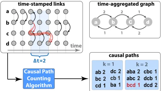
We consider a set D of (directed) time-stamped links (s, d, t) ∈ V ×V ×N where s, d ∈ V are the source and target node of the link respectively, and t∈N is the discrete time stamp of an instantaneously occurring link (s, d) (see left panel in Fig. 1). We call a sequence
p:=n# ”0n1. . . nl
of nodesni ∈V acausal path for a maximum time differenceδ ∈Niff ∀i∈ {0, . . . , l−1} 1. ei:= (ni, ni+1, ti)∈D,
2. ti+1 > ti, and 3. ti+1−ti ≤δ
We highlight that the second condition in the definition above forces sequences of time-stamped links on a causal path to respect the chronological order. Ignoring this restriction would lead to a definition of paths by which nodes can influence each other backwards in time. For any δ <∞, the third condition limits the maximum time difference between any two consecutive links on a causal path. Clearly, different systems require different values for δ, e.g. for the propagation of rumours in social networks the value of δ is linked to the “memory” of actors, while for the propagation of an epidemic it is linked to the time to recovery from an infectious disease. The detection of the optimal time scaleδ to analyse a given data set is an important problem by itself [9] that we do not address, i.e. for the purpose of our work, we treat the parameter δ as given.
We further define the length kpk of path p = n# ”0n1. . . nl as the number l of traversed links. Moreover, we call any sequence of time-stamped links (e0, . . . , el−1) that constitute a causal path
p one instance of the causal path p in D. With this, we formulate the problem addressed by our algorithm: Given a data set Dof time-stamped links, a maximum time differenceδ, andK ∈N we want to calculate the number of instances C(p) of all causal paths p with kpk ≤K. Formally, we define
C(p) =|{(e1, . . . , ek)|(e1, . . . , ek) is an instance of p in D}|
A toy example for a set of time-stamped linksDand the resulting outputC(p)forδ = 2andK= 2 is shown in Fig. 1. For illustrative purposes, in the left panel of Fig. 1 we show a so-called time-unfolded representation of a temporal network, where each node is represented by multipletemporal copies. We note that for a maximum time difference of δ = 2 time units, this example contains two instances ((a, b,1),(b, c,3))and((a, b,2),(b, c,3))of the causal pathabc# ”and thusC(abc# ”) = 2. This captures the fact that, e.g., an epidemic can spread in two different ways from node avia node
b to node c.
The rationale behind our definition ofC(p) – and thus the motivation of our work – is that we want to count in how many different ways nodes can (indirectly) influence each other in a temporal network. It provides a natural generalisation ofweighted links, which count instances of time-stamped links in time-aggregated network models [4]. Since each time-stamped link is an instance of a causal path with length one, C(p) extends the notion of link weights to causal paths of arbitrary length. This is an important basis to generalise static network models to higher-order models [5].
Causal Path
Counting
Algorithm
2 2 2 1 1 1aba
2
abc
2
bcd
1
time-stamped links
causal paths
k = 1
ab
2
bc
2
cd
1
Δt=2k = 2
a
b
c
d
time
time-aggregated graph
dc
2
cb 1
ba
1
cbc
1
dcb
1
dcd
2
a b C dFigure 1: For a set of time-stamped links between nodes in a graph, our algorithm efficiently counts
causal paths up to a given length K (right) for maximum time difference δ. In the example above, for δ = 2 the time-stamped links (b, c, t = 3) and (c, d, t = 5) contribute to a causal path bcd# ” of length two, of which a single instance occurs in the data.
Related Work Approaches to find patterns in temporal networks that are related to our work exist in several research areas, namely (i) works using time-respecting paths in temporal network analysis, (ii) approaches calculating or estimating the statistics of paths as a basis for higher-order network models, and (iii) methods to efficiently analyse so-called network motifs in temporal data.
Algorithms to calculate causal or time-respecting paths in area (i) have generally focused on generalisations of path problems in graph theory to temporal networks [10]. As such, most works in this line of research have considered algorithms to compute shortest or fastest causal paths [11], the accessibility of nodes via causal paths with at most length k [12, 13], or the generalisation of path-based centralities to causal paths in temporal networks [14].
While the works in area (ii) are an important motivation for our algorithm they have not focused on algorithmic aspects of efficiently counting causal paths. They have thus either used heuristic approaches to generate causal path statistics based on simple stochastic models [15] or adopted simple algorithms that do not scale to large data sets [16].
Taking a different perspective, counting paths in a temporal network can be considered a special case of counting temporal motifs [17]. We highlight that, while the causal paths counted by our method for a given K andδ are necessarily K-edge K·δ temporal motifs as defined, e.g., in [17], the opposite is not true. Hence, our work focuses on a computational problem that, while being less general then the problem of counting arbitrary temporal motifs, is nevertheless of crucial importance to studycausal topologies in temporal networks. To the best of our knowledge, our work is the first to provide a fast streaming algorithm to count causal paths in temporal networks for given maximum time differenceδ and maximum path lengthK.
3
Counting Causal Paths
We now introduce an efficient streaming algorithm, which counts all instances of causal paths of lengths k ≤ K for a given maximum path length K and a maximum time difference δ between subsequent links on causal paths (cf. section 2). It uses an iterative approach that incrementally extends causal paths by moving a sliding time window of lengthδ over the data. Initially, each time-stamped link (n1, n2, t) is a causal path n# ”1n2 of length one that can be extended by time-stamped links in time window(t, t+δ]. To denote the extension of a causal path, we define a binary operator
⊕on a path n# ”0. . . nk and a node nk+1 as follows:
# ”
n0. . . nk⊕nk+1 :=n# ”0. . . nknk+1
We assume that the time-stamped links in the dataDare chronologically ordered, whereei refers to thei-th link in the ordered sequence. Our proposed algorithm performs a single pass through this sequence and, for each time-stamped linkei, computes the countCi of causal path instances ending with link ei. We define Ci(p) := m, where m counts different instances of causal path p that end with ei.
To calculate the output C, we iteratively aggregate path counters Ci by a simple addition, i.e. we sum two path counters C andC0:
Csum =C+C0 ⇐⇒ ∀p:Csum(p) =C(p) +C0(p)
We denote the operationextK(C, n)that takes a path counterC and nodenand extends each path in C with n, thus obtainingCext:
Cext=extK(C, n) ⇐⇒ ∀p,kpk< K:Cext(p⊕n) =C(p)
Our method can now be formulated as shown in Algorithm 1. We explain it step-by-step and illustrate it in Fig. 2, using the toy example from Fig. 1. We assume time-stamped links to be stored in a listD with length N, while δ and K are integers. We further assume that the path counts Ci as well as the overall output C are implemented as dictionaries ci and c respectively, which have causal paths p as keys and integer counts as values. We do not store paths whose count is zero. In lines 1 and 2 we initialise the path count dictionary c as well as the time window W. In line 3 we iterate through the ordered sequence of time-stamped links (s, d, t). In each iteration we first initialize the dictionaryci that representsCi (line 5). Since a time-stamped link (s, d, t) is a causal path sd#” of length one we set its counter to one (line 6). We then iterate through the time window
W (line 7 and 8), which contains tuples(sj, dj, tj, cj)representing all time-stamped links (sj, dj, tj) and causal path counts cj that could be continued as a causal path by link (s, d, t). The red box in Fig. 2 highlights the time-stamped links and path counts in time window W at iteration i = 6 for δ = 2. If the time-stamped link (sj, dj, tj) in the time-window is outdated (lines 9 and 10), we
Algorithm 1 Calculate occurrences of all causal paths in data D that are at most K steps long, assuming parameter δ Require: D,δ, K 1: c←dict() 2: W ←list() 3: foriin 1toN do 4: (s, d, t)←D[i] 5: ci←dict() 6: ci[sd#”]←1 7: for j in1toW.length()do 8: (sj, dj, tj, cj)←W[j] 9: if tj< t−δthen 10: W ←W.remove((sj, dj, tj, cj)) 11: else 12: if dj =s∧t > tj then 13: for pincj.keys() do 14: ifkpk< K then
15: if p⊕dnot inci.keys()then
16: ci[p⊕d]←cj[p]
17: else
18: ci[p⊕d]←ci[p⊕d] +cj[p]
19: for pinci.keys()do
20: if pnot inc.keys()then
21: c[p]←ci[p]
22: else
23: c[p]←c[p] +ci[p]
24: W.append((s, d, t, ci))
25: return C
remove both the link and its dictionary cj fromW. Otherwise, if a time-stamped link (sj, dj, tj) in
W is continued by(s, d, t)(lines 11 and 12) each causal pathpthat ends with(sj, dj, tj)is extended by node d. We thus found new causal paths p⊕dand update ci such that Ci ←Ci+extK(Cj, d) (lines 13-18). We next updatecsuch thatC←C+Ci (lines 19-23) and extend the window by one time-stamped link D[i]and path countsci (line 24). Once we have completed a single pass over the time-stamped links, the dictionaryc contains counts of all causal path instances with length k≤K
and maximum time difference δ.
Computational Complexity In the following, we briefly comment on the computational complexity of our algorithm.
Assuming that the maximum number of links in the time window ismδ for δ <∞, and that the input sequenceDis ordered, the computational complexity of our method isO(N|V|K2[mδλKmax−2+
λKmax]), where λmax is the largest eigenvalue of the binary adjacency matrix of the time-aggregated network G = (V, E). We note that the maximum eigenvalue λmax is called algebraic connectivity and is linked to the sparseness of a graph topology. λmax takes a maximum value of|V|for a fully connected graph G= (V, E). For the special case ofδ → ∞,mδ scales asN and the scaling is at most quadratic in the size of the input sequence D.
For the more detailed derivation of the bounds above, we first consider that the maximum number of links that have the same time-stamp t is bounded above by a constant m for all t. The upper bound for the number of links in any time window is then mδ = mδ for δ < ∞. Assuming the number Λ(K) is the upper bound for the possible number of causal paths with length up to K
computational complexity is:
O(N ·K·[mδδΛ(K−2) + Λ(K)])
i si di ti ci 0 a b 1 ab#”: 1 1 a b 2 ab#”: 1 2 b a 3 ba#”: 1,aba# ”: 2 3 b c 3 bc#”: 1,abc# ”: 2 4 d c 3 dc#”: 1 5 d c 4 dc#”: 1 6 c d 5 cd#”: 1,bc# ”d: 1,dc# ”d: 2 7 c b 6 cb#”: 1,dcb# ”: 1 8 b c 7 bc#”: 1,cbc# ”: 1
Figure 2: Illustration of one iteration of our algorithm in the example shown in Fig. 1. The left columns contains the data, while the right column shows path counters ci for δ = 2and maximum path length K = 2. The red box shows time window W of links that could be continued by the considered link (iteration i = 6, highlighted in blue). The right column shows causal path counts stored in ci after iteration i= 6, with paths fromW extended in i= 6 shown in red.
of the underlying graph. The maximum number of paths on a time-aggregated, directed graph is bounded above by the number of paths in its undirected version G. We can thus derive an upper bound for Λ(K) based on the topology of the time-aggregated, undirected, graph G = (V, E) of time-stamped links in D. We note that the number of paths of length k in a graph G can be calculated as
X
i,j
(Ak)ij,
whereAis the binary adjacency matrix ofGandAkis thek-th matrix power of A. AssumingAis positive semi-definite, we can decompose it toA=QΛQT whereΛis a diagonal matrix, consisting of positive eigenvalues. We can decompose Λto Λ=√Λ√Λ, and insertQTQ=1 in between:
A=Q
√
ΛQTQ
√
ΛQT
We denoteQ√ΛQT asS, thereforeA=STS. The maximum eigenvalue ofS,λmax(S)is equal to the square root of λmax(A). Then, by the definition of the induced norm for matrices, we have:
∀x,kSk2> kSxk2 kxk2 SincekSk2 =λmax(S),kSxk2 = √ xTSTSx andkxk 2 = √ xTx we have: q
λmax(A) =λmax(S)>
√
xTSTSx
√
xTx
In particular for x= (1,1,1, . . . ,1)T, where xis n-dimensional, andxTx=n: q λmax(A)> q P i,jSTS √ n = q P i,jAi,j √ n Thus nλmax(A)> X i,j Ai,j
We can can thus derive an upper bound for the number of paths of lenth k: X
i,j
Akij ≤ |V| ·λkmax
where λmax is the largest eigenvalue of the adjacency matrix A, which is also called the algebraic
connectivity of a graph. ForΛ(K) we thus obtain
Λ(K) = K X l=1 X i,j Alij ≤ K X l=1 |V| ·λlmax
Assuming λmax>1, we find the upper bound:
ON · |V| ·K2·hmδδλKmax−2+λKmax
i
We note that the worst case complexity holds for a fully connected graph, where all sequences of k
nodes constitute a possible causal paths of lengthk. In this case we haveλmax =|V|and the upper bound is
ON ·K2·hmδ·δ· |V|K−1+|V|K+1 i
In the extreme case of δ = ∞, mδ scales as N and the complexity of our algorithm thus scales quadratically with N, i.e.
ON ·K2·hN · |V|K−1+|V|K+1i.
This shows that, for any finite maximum time differenceδ used in the definition of causal paths, the runtime of our algorithm scales linearly with the size of the data N. The multiplicative factor in the term grows exponentially with the maximum causal path length K, with the base that depends on the sparsity of the graph captured in the leading eigenvalue. We finally highlight that in real-world settings we are typically interested in causal path statistics for small values of K, corresponding to the maximum order of higher-order graphical models of causal paths.
4
Experimental Results
We present results of preliminary experiments in which we asses the runtime of our algorithm for different sizes N of data, for different maximum time differences δ, and for different values of the maximum lengthK of causal paths. We compare the runtime of our method to a baseline algorithm, which has been used to compute causal paths in time-stamped data [16]. We chose this baseline since (i) other works focus on computingshortest causal paths, which is a different problem, and (ii) it is available in the Open Source package pathpy1. To count causal paths, the baseline algorithm performs three steps: First, adopting an approach similar to [10], time-stamped links are represented as direct acyclic graph (DAG). Second, the DAG is used to compute all causal paths between root and leaf nodes. And third, all shorter paths of length k contained in those longest causal paths are counted. Different from the sliding window approach of our method, this algorithm is not suitable for streaming scenarios.
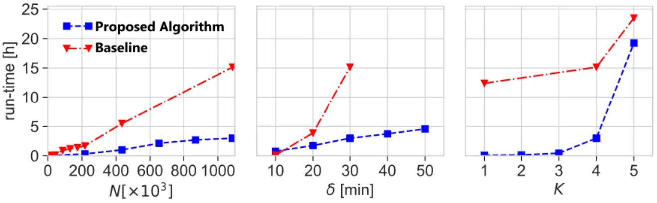
We assess the runtime of our algorithm in empirical data capturing time-stamped proximities between students, which was collected by the RealityMining project [18]. It captures N = 1086404 time-stamped links over a period of more than six months between |V| = 96 nodes. Due to the density of the data, calculating causal paths in this data is challenging with the baseline algorithm, in particular as δ increases.
Fig. 3 shows the results of our preliminary experiments. The left panel shows the runtime for a fixed value of δ that corresponds to 30 minutes, and a fixed maximum causal path length K = 4.
1
We show the dependency of the runtime on the size N of the data by running the algorithm on the first N time-stamped interactions in the RealityMining data set. The results clearly show that our approach outperforms the baseline algorithm for all values of N. They further support the linear scalability of our algorithm found in section 3.
The middle panel shows the dependency of the runtime on the maximum time difference δ for
K = 4. Supporting the theoretical analysis in section 3, we find that the runtime of our algorithm linearly depends on δ. Due to the calculation of causal paths between root and lead nodes in the DAG, the runtime of the baseline algorithm superlinearly grows withδ, which makes it unsuitable for big data. For the baseline algorithm we had to skip values of δ larger than 30 minutes due to the prohibitively long runtime of those experiments.
Finally, the results in the right panel show the dependency of the runtime on the maximum length
K of causal paths. The result again supports our theoretical analysis, which yields a multiplicative factor that exponentially scales in K. We highlight that this exponential scaling in K is due to the growth of the output calculated by our algorithm, i.e. the number of causal paths of length up to
K that can exist in the data.
Proposed Algorithm Baseline
Figure 3: The left panel shows how runtime (y-axis) depends on the number of time-stamped links
N (x-axis) for fixed values of δ = 30 minutes and K = 4. The middle panel shows how the time needed to process the whole data (y-axis) for fixed K = 3 depends on δ (x-axis). The right panel shows how the runtime depends onK for fixedδ= 30 minutes.
5
Discussion and Outlook
Causal paths are crucial to understand how nodes in systems with time-varying topologies indirectly influence each other. This has recently been identified as an important problem in the study of time series data on complex networks [5]. Fast methods to count causal paths are needed to fit and select higher-order models, detect paths with anomalous frequencies, model diffusion and epidemic spreading, rank nodes based on centralities, and detect clusters in big time series data on networks. To this end, we present a fast streaming algorithm to count causal paths in temporal networks. The results of our preliminary experiments (i) confirm our theoretical analysis of scalability, and (ii) show that it outperforms a baseline algorithm implemented in an OpenSource package. Since both the baseline method and our proposed algorithm are deterministic, our experimental results are based on a single run in a single data set. More experiments are thus needed to substantiate our findings in a larger number of big time series data. Our method further has considerable parallelisation potential, which we will explore in future work. In the light of these perspective, our work is a promising first step towards scalable data mining techniques for temporal network data.
References
[1] Page, L., Brin, S., Motwani, R. & Winograd, T. The pagerank citation ranking: Bringing order to the web. Technical Report 1999-66, Stanford InfoLab (1999). URL http://ilpubs. stanford.edu:8090/422/.
[2] Rosvall, M. & Bergstrom, C. T. Maps of random walks on complex networks reveal community structure. Proceedings of the National Academy of Sciences 105, 1118–1123 (2008).
[3] Grover, A. & Leskovec, J. node2vec: Scalable feature learning for networks. In Proceedings of the 22nd ACM SIGKDD international conference on Knowledge discovery and data mining, 855–864 (ACM, 2016).
[4] Holme, P. Modern temporal network theory: a colloquium. The European Physical Journal B
88, 234 (2015).
[5] Lambiotte, R., Rosvall, M. & Scholtes, I. From networks to optimal higher-order models of complex systems. Nature Physics 15(2019).
[6] Scholtes, I. et al. Causality-driven slow-down and speed-up of diffusion in non-markovian tem-poral networks. Nat. Comm.5, 5024 (2014).
[7] Rosvall, M., Esquivel, A. V., Lancichinetti, A., West, J. D. & Lambiotte, R. Memory in network flows and its effects on spreading dynamics and community detection. Nature communications
5, 4630 (2014).
[8] Xu, J., Wickramarathne, T. L. & Chawla, N. V. Representing higher-order dependencies in networks. Science advances 2, e1600028 (2016).
[9] Caceres, R. S. & Berger-Wolf, T. Temporal scale of dynamic networks. In Temporal Networks, 65–94 (Springer, 2013).
[10] Kempe, D., Kleinberg, J. & Kumar, A. Connectivity and inference problems for temporal networks. InProceedings of the thirty-second annual ACM symposium on Theory of computing, 504–513 (ACM, 2000).
[11] Wu, H.et al. Path problems in temporal graphs. Proceedings of the VLDB Endowment (2014).
[12] Whitbeck, J., Dias de Amorim, M., Conan, V. & Guillaume, J.-L. Temporal reachability graphs. In Proceedings of the 18th Annual International Conference on Mobile Computing and Net-working, Mobicom ’12 (2012).
[13] Lentz, H. H. K., Selhorst, T. & Sokolov, I. M. Unfolding accessibility provides a macroscopic approach to temporal networks. Phys. Rev. Lett.110, 118701 (2013).
[14] Takaguchi, T., Yano, Y. & Yoshida, Y. Coverage centralities for temporal networks. The European Physical Journal B 89, 35 (2016).
[15] Salnikov, V., Schaub, M. T. & Lambiotte, R. Using higher-order markov models to reveal flow-based communities in networks. Scientific reports 6, 23194 (2016).
[16] Scholtes, I. When is a network a network?: Multi-order graphical model selection in pathways and temporal networks. In Proceedings of the 23rd ACM SIGKDD International Conference on Knowledge Discovery and Data Mining (2017).
[17] Paranjape, A., Benson, A. R. & Leskovec, J. Motifs in temporal networks. In Proceedings of the Tenth ACM International Conference on Web Search and Data Mining, 601–610 (ACM, 2017).
[18] Eagle, N. & (Sandy) Pentland, A. Reality mining: sensing complex social systems. Personal and Ubiquitous Computing 10, 255–268 (2006).