research paper series
Globalisation and Labour Markets
Research Paper 2007/30
Oligopoly, open shop unions and trade liberalisation
by
Paulo Bastos, Udo Kreickemeier and Peter Wright
The Authors
Paulo Bastos is a Postdoctoral Research Fellow in the Leverhulme Centre for Research on
Globalisation and Economic Policy (GEP), University of Nottingham; Udo Kreickemeier is an
Associate Professor in the School of Economics, University of Nottingham, and an Internal
Fellow in GEP; Peter Wright is an Associate Professor and Reader in the School of Economics,
University of Nottingham, and an Internal Fellow in GEP.
Acknowledgements
We would like to thank Rod Falvey, Kjell Erik Lommerud, and participants at the Royal
Economic Society annual conference in Nottingham, European Trade Study Group annual
conference in Dublin, Spring Midwest International Economics Meetings in Lawrence-Kansas
and seminars at the University of Porto and NIPE-University of Minho for helpful comments.
Financial support from the Leverhulme Trust (Programme Grant F114/BF) is gratefully
acknowledged. Paulo Bastos thanks Fundacao para a Ciencia e a Tecnologia for financial
support. A previous version of this paper was circulated under the title ‘Open Shop Unions and
International Trade Liberalisation.’
Oligopoly, open shop unions and trade liberalisation
by
Paulo Bastos, Udo Kreickemeier and Peter Wright
Abstract
In an international oligopoly model, we investigate how trade liberalisation impacts on collective bargaining outcomes when workers are represented by open shop unions. We find that, with intermediate levels of union density, trade liberalisation may lead to higher negotiated wages even if no trade occurs in equilibrium. In addition, we show that union wages may be higher with free trade than in autarky.
JEL classification
: F15, J5, L13
Keywords
: International oligopoly, bargaining, open shop unions, trade liberalisation.
Outline
1.
Introduction
2.
The model
Non-Technical Summary
In spite of the well known potential benefits for aggregate welfare, the labour market effects of trade
liberalisation appear to have become a major source of anxiety in recent years. In the European Union, for
example, negative perceptions towards increased globalisation were pointed out as one of the main
reasons for the recent rejection of the European constitution by French and Dutch voters (Niblett, 2005).
Additionally, opinion polls undertaken in the older member states point to a rising anti-European attitude,
reflecting in part concerns that the European Union may be amplifying the threats of globalisation by
opening borders to cheaper labour and cheaper products from the Eastern neighbours (Dempsey, 2005).
Within this debate, the spectre that freer trade induces trade unions to engage in a race-to-the-bottom in
wages is a particular cause of concern. At the same time, perhaps conflicting with the race-to-the-bottom
argument, collective bargaining institutions continue to be regarded as a major source of downward wage
rigidity, which will potentially generate macroeconomic imbalances as globalisation proceeds.
How might we expect trade liberalisation to impact on collective bargaining outcomes? In this paper we
investigate this question by means of an international duopoly model in which organised labour seeks to
capture a share of the quasi-rents obtained by its employer. Like most of the existing literature, we model
the process of integration as a gradual reduction in the per unit cost incurred by each firm when exporting
to the other country. The main novelty here is that, rather than wages being set unilaterally by monopoly
unions, they are the outcome of a Nash bargaining process in which the fallback position of the firm
depends on the level of trade union density. This framework allows us, therefore, to capture an important
aspect of reality.
We show that, when union density is less than 100%, trade liberalisation impacts on bargained wages
through a previously unnoticed mechanism. Harsher international competition (actual or potential) reduces
the fallback position of the firm in the event of a strike, which serves to help the union in the bargain. In
other words, a labour dispute at home induces a competitive response from the overseas rival, making the
conflict more costly to the local firm. For this reason, the firm is willing to sacrifice a larger share of its
quasi-rents in order to preclude such a dispute. The implications of this mechanism for the impact of trade
liberalisation on wages are profound: firstly, trade liberalisation may lead to higher bargained wages even
if no trade exists in equilibrium; secondly, wages need not fall in absolute terms as the economy moves
from autarky to free trade.
1
Introduction
In spite of the well known potential benefits for aggregate welfare, the labour market effects of trade liberalisation appear to have become a major source of anxiety in recent years. In the European Union, for example, negative perceptions towards increased globalisation were pointed out as one of the main reasons for the recent rejection of the European constitution by French and Dutch voters (Niblett, 2005). Additionally, opinion polls un-dertaken in the older member states point to a rising anti-European attitude, reflecting in part concerns that the European Union may be amplifying the threats of globalisation by opening borders to cheaper labour and cheaper products from the Eastern neighbours (Dempsey, 2005). Within this debate, the spectre that freer trade induces trade unions to engage in a race-to-the-bottom in wages is a particular cause of concern.1 At the same
time, perhaps conflicting with the race-to-the-bottom argument, collective bargaining in-stitutions continue to be regarded as a major source of downward wage rigidity, which will potentially generate macroeconomic imbalances as globalisation proceeds.
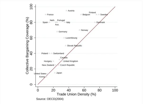
How might we expect trade liberalisation to impact on collective bargaining outcomes? In this paper we investigate this question by means of an international duopoly model in which organised labour seeks to capture a share of the quasi-rents obtained by its employer. Like most of the existing literature, we model the process of integration as a gradual reduction in the per unit cost incurred by each firm when exporting to the other country. The main novelty here is that, rather than wages being set unilaterally by monopoly unions, they are the outcome of a Nash bargaining process in which the fallback position of the firm depends on the level of trade union density. This framework allows us, therefore, to capture an important aspect of reality: As illustrated in Figure 1, trade union density varies considerably across countries, and is typically lower than collective bargaining coverage.2
We show that, when union density is less than 100%, trade liberalisation impacts on bargained wages through a previously unnoticed mechanism. Harsher international competition (actual or potential) reduces the fallback position of the firm in the event of a strike, which serves to help the union in the bargain. In other words, a labour dispute
1Concerns over this issue among the policymaking community are apparent in recent publications of
the OECD (2004, 2005a,b) and European Commission (2005). The importance of this matter for organised labour is evident in ongoing discussions within the trade union movement about the implications of deeper integration for the wage and employment prospects of their members (see, for example, the website of the European Trade Union Confederation, www.etuc.org)
2In reality, open shop arrangement, where the union is recognised for bargaining purposes but
member-ship is not compulsory, are the dominant form of union organisation in most European countries (OECD, 2004).
Aus. Austria Belgium Canada Czech Republic Denmark Finland France Germany Hungary Italy Japan Korea Luxembourg Neth. New Zealand Norway Poland Portugal Slovak Republic Spain Sweden Switzerland United Kingdom United States 0 20 40 60 80 100
Collective Bargaining Coverage (%)
0 20 40 60 80 100
Trade Union Density (%) Source: OECD(2004)
Figure 1: Union density and coverage in the OECD in 2000 (percentage of wage and salary earners)
at home induces a competitive response from the overseas rival, making the conflict more costly to the local firm. For this reason, the firm is willing to sacrifice a larger share of its quasi-rents in order to preclude such a dispute. The implications of this mechanism for the impact of trade liberalisation on wages are profound: firstly, trade liberalisation may lead to higher bargained wages even if no trade exists in equilibrium; secondly, wages need not fall in absolute terms as the economy moves from autarky to free trade.
This paper builds on the work of several predecessors. In an international duopoly model with monopoly unions in both countries, Huizinga (1993) finds that the wage level is lower with free trade than in autarky. This is because, although market expansion as a result of trade liberalisation causes wages to rise, this is more than offset by the increased product market competition which serves to moderate wages. In two influential papers, Naylor (1998, 1999) argues however that the conclusion that trade liberalisation leads to wage reductions is a special, rather than a general, case and results from a comparison of polar ends of the possible range of trade regimes. Modelling the process of integration
as a marginal reduction in trade costs, he arrives at the striking conclusion that, within a context of two-way trade, further liberalisation reduces the labour demand elasticity which leads to unionised labour setting higher wages i.e. with two-way trade, the market expansion effect dominates the market discipline effect. Note however that wages under free trade are still lower than those under autarky.3
Various extensions of Naylor’s results have been made. Munch and Skaksen (2002) distinguish between fixed and variable trade costs when both labour markets are unionised. They conclude that while a fall in fixed trade costs leads to an unambiguous fall in wages, the implication of a reduction in variable costs is ambiguous. Piperakiset al. (2003), unlike Naylor (1998), allow for asymmetry between the countries. They show that if the market size of the two countries differs widely, a reduction in trade costs can lead to decreases in wages, employment and welfare in the country with the larger market. This is because the larger economy has less to gain, relatively speaking, from the market expansion effect. The paper by Lommerud et al. (2003) then shows that if one country is unionised and the other is not, a much wider range of trade regimes is possible than previously considered. Under autarky, all trade is prevented by the level of trade costs, and wages are set in isolation in each country. However, as trade costs fall, the ability of organised labour to obtain higher wages in the unionised country will be limited by the possibility that firms from the low wage (non-unionised country) will begin to export. This leads to what Lommerudet al. (2003) call theimport deterrenceregime. If liberalisation continues, trade costs will eventually fall to such an extent that trade begins and the foreign firm starts to export. One-way trade then continues until trade costs fall to a level such that the unions find it in their best interests to adopt a low wage strategy in order to induce the domestic firm to export as well. Under two-way trade, Naylor’s result prevails as the market expansion associated with further liberalisation causes wages to rise. As with the preceding papers, however, wages are shown to be higher in autarky compared with free (or indeed one-way) trade.4
A common feature of the literature reviewed above is the adoption of the monopoly
3The movement from autarky to two-way trade is triggered when the unions in the two countries find
it optimal to abandon their previous high wage strategies, and instead lower their wage demands in order to allow their firms to compete internationally. This causes a discontinuity in the wage level, as union demands are adjusted downwards. However the union gains from the rapid expansion in employment that results. The wage fall, as the union discretely moves from a high wage strategy to a low wage strategy, outweighs any subsequent expansion in wages.
4Within this framework Lommerud et al. (2003) then examine how wage setting impacts on the location
decisions of multinational firms. They argue that if the firm has plants located in both countries then this would serve to simplify the wage schedules, since the union no longer gains by adopting a low wage strategy in order to induce its plant to export. Thus wages fall continuously from autarky to free trade. More generally, the option of locating abroad serves to weaken the position of the union.
union model to characterise wage determination in unionised sectors. Within such setting, equilibrium wages are governed by the elasticity of labour demand with respect to the wage rate. Therefore, trade liberalisation impacts on wages if and only if it affects the trade-off between wages and employment faced by the union. The present paper extends this literature by adopting a framework in which wages are the outcome of a Nash bargain between a firm and an open shop union. Since a firm may continue to operate with its non-union workers in the event of a strike, its fallback position depends on union density. The possibility also exists that the foreign rival will export to meet a shortfall in product supply as a result of a strike, which acts as a discipline on the firm and serves to boost the union’s position. Thus, unionised wages may rise with trade liberalisation even if no trade occurs in equilibrium. This is what we call theimport threat regime, which is new to the literature.
In contrast to the previous literature, wages may also be higher with free trade than under autarky. With low levels of density the union is only able to capture a small proportion of the relatively large surplus under autarky. Its position under free trade is stronger. Although the surplus to be bargained over is smaller, a strike not only causes disruption to production but also elicits a competitive response from the overseas firm. This reduces the firm’s strike profits further and serves to bolster the position of the union. Hence, when workers are represented by open shop unions, wages need neither fall monotonically as trade liberalisation occurs, nor indeed to fall in absolute terms as an economy moves from autarky to free trade.
The remainder of the paper is organised as follows. Section 2 presents the basic model setup and solution. Section 3 then analyses the impact of reductions in trade costs on negotiated wages, for different levels of union density. In Section 4 we discuss some extensions of our model. Section 5 concludes.
2
The model
2.1 Basic setup
Consider an international duopoly industry. Firm 1 is located in country 1 and firm 2 in country 2. The firms produce a homogeneous commodity under constant returns to scale with labour as the only input, and output per worker being normalised to unity. Product demand is linear, with the inverse demand function in countryigiven by:
where, a, b >0,pi is the price in country i and yii and yij denote, respectively, the sales of the firm located in country i to markets i and j. In line with Brander (1981), we assume that each producer views each country as a separate market and that there is a constant trade cost of tper unit of commodity exported. Competition in the two markets is Cournot.
In country 2 the firm recruits workers from a competitive labour market at a wage rate
wc
2, which for simplicity is normalised to zero. In country 1, there is a single open shop
union that represents all workers employed at firm 1.5 Union densityµcan vary between 0
and 1. All workers covered by the union receive the same bargained wagew, independent of their membership status.6
Union density is exogenously given when collective bargaining takes place. Therefore, we are implicitly assuming that the individual decision to become a union member is independent of wage formation. Here we note that this assumption is consistent with the literature on open shop unions. Since the bargained wage is a pure public good and union membership involves a private cost (the membership fee), there is a free-rider problem associated with the individual decision to become unionised. In order to explain voluntary union membership in the context of an open shop union, the existing literature typically assumes that the union provides a private good to its members. Examples of this excludable good, available only through membership, are privileged access to grievance procedures or reputation gains from complying with a social custom. The valuation of these benefits are assumed to vary across individuals, and a worker will become a union member if the utility gain associated with the private good provided by the union more than compensates for the utility loss caused by the membership fee. In this context, the individual membership decision may be independent of the collective wage.7
In country 1, there is also a perfectly competitive sector where workers can earn the
5Examples of international oligopoly models in which the labour market is unionised in one country and
perfectly competitive in the other include Lommerudet al. (2003, 2006) and Straume (2003). The model could be extended by allowing for an industry-level open shop union covering workers inn >1 domestic firms. Whilst that would change our quantitative results, it can be shown that it would not affect our main qualitative findings.
6The pure public good nature of the bargained wage is a distinctive feature of open shop unions - see,
for example, Naylor and Cripps (1993) and Naylor and Rauum (1993).
7Naylor and Cripps (1993) and Booth and Chatterji (1995) argue that membership is increasing in
the collective wage. This result, however, hinges on the assumption that the indirect utility function of each worker is concave, which guarantees that the utility loss by paying the membership fee is decreasing in the wage. Under this assumption, a higher wage ensures that even workers that place a relatively low valuation on the union excludable good rationally decide to become union members. However, this (restrictive) assumption is not common to all papers on ‘open shop’ unions. Naylor and Rauum (1993), Corneo (1993, 1995) assume that the marginal utility of income of each member is constant, which implies that the individual decision to become a union member is independent of the collective wage.
competitive wagewc
1 =wc2= 0. Profits for the two firms are given by:
π1= [a−b(y11+y21)−w]y11+ [a−b(y22+y12)−w−t]y12 (2)
π2= [a−b(y22+y12)]y22+ [a−b(y11+y21)−t]y21 (3)
Following Naylor and Cripps (1993) and Naylor and Raaum (1993), we consider a sequence of contract periods. In the event of a strike the firm is able to employ only that fraction of its workers who are not union members under the terms of the contract negotiated in the previous period, and furthermore that the firm neglects the impact of its current employment decisions on future wage negotiations.
Denote the output of firm 1 in marketjin the previous contract period byy1j.8 Under
these assumptions, when firm 1 only supplies the home market, its output under a strike is given by ys
11= (1−µ)y11, while it is given by ys11+ys12= (1−µ) (y11+y12) if firm 1
serves both markets.9 Firm 1’s profits in case of a strike are then given by
π1s= [a−b(y11s +y21s )−w]ys11+ [a−b(ys22+y12s )−w−t]y12s , (4) where w is the wage rate negotiated in the previous contract period andys
2j is the sales
volume of firm 2 in market j in the case of a strike in firm 1.
We adopt a standard right-to-manage model where the firm is allowed to set employ-ment to maximise profits given the wage. In each contract period, the outcome is modelled as a two-stage game. In Stage 1 the unionised firm and bargains over wages through a Nash bargaining process, for a given level of union density. In Stage 2, both firms decide on their level of production, and hence employment, taking as given the wage of the other firm and taking into consideration their labour demand schedule. In order to solve the model analytically, we proceed by backwards induction. We begin by examining Stage 2 and solve for the optimal production decisions of the firms. Once these are known we can examine Stage 1, and solve for the steady-state wage level that results from the wage bargain.
8That is, firm 1’s profit maximising level of output for marketj, given the wage rate negotiated in the
previous contract period.
9In the case of a strike, the firm may find it optimal to reallocate output across markets, and hence in
generalys
2.2 Solving for production
Solving the first order conditions for profit maximisation yields the standard reaction functions of both firms:
y11= a−2bw −12y21 (5) y12= a−2wb−t−12y22 (6) y21= a−t 2b − 1 2y11 (7) y22= 2ab− 12y12 (8)
In order to obtain the equilibrium levels of output for each firm in each market, we can solve eqs. (5) to (8) simultaneously. Given the constraint that all production quantities have to be non-negative, this yields the following solutions for equilibrium sales:
y11, y21= ( 1 2b(a−w),0 1 3b(a−2w+t),31b(a+w−2t) ift≥et(w) ift <et(w) (9) y22, y12= ( 1 2ba,0 1 3b(a+t+w),31b(a−2t−2w) ift≥bt(w) ift <bt(w) (10)
with et(w) = (a+w)/2 and tb(w) = a/2−w. Boundary et(w) separates the no-trade and one-way trade regimes, whilebt(w) separates the one-way trade and two-way trade regimes. While the boundaries between trade regimes are therefore dependent on the endogenous wage rate, the outcome of the wage bargain in turn depends on which trade regime we are in. In order to solve this problem of mutual dependency, we proceed as follows: We exogenously specify the respective trade regime, solve the regime-specific bargaining problem and use the resulting wage rates to express the regime boundaries in terms of model parameters.
2.3 Solving the wage bargain
In stage 1, the wage paid by the firm in country 1 is modelled as the outcome of a Nash bargain between the firm and its union:
wr= arg max
w [(U1−U s
where superscriptrdenotes the respective trade regime. Union utility is given byU1, while
Us
1 is the disagreement payoff of the union. For simplicity, we assume that the objective
of the union is to maximise wages, and so by implication, U1s is the wage in event of a strike.10 The strike pay is assumed to be exogenous, and it is set equal to zero without
further loss of generality.11
In the absence of international trade, π1 is given by eq. (2), with y12 =y21 = 0 and
y11substituted from eq. (9). In order to fully specify the Nash bargain we need to findπ1s,
the unionised firm’s profits in the event of a strike. Given that output of firm 1 is reduced during a strike, it is possible that firm 2 would start exporting i.e. y21s could be positive, even with y21 = 0. From eq. (9), firm 1’s production in the event of a strike is given by
ys
11 = (1−µ)(a−w)/(2b), and substitution into the reaction function for firm 2, eq. (7),
yieldsys21= (a(1 +µ) +w(1−µ)−2t)/(4b). The value forπs1 is found by substituting into eq. (4).
The situation whereys
21 is strictly positive is labelled theimport threat (it) case. Even
though there is no trade in equilibrium, the fact that firm 2 will export in the event of a strike affects πs
1 and hence the outcome of the bargaining process. It is easily checked
that ys
21≥0 holds for
t≤ a(1 +µ) +w(1−µ)
2 (12)
Fortabove the threshold, what we call thepure autarky (a) case, the disagreement payoff is given by eq. (4) with ys
12 =y21s = 0, since the high trade costs preclude any impact of
the foreign firm on the domestic firm’s conflict payoff. To solve the wage bargain in both regimes, we substitute for π1 and πs
1 in eq. (11), and useU1 =w and U1s = 0. In the first
order condition for a maximum, we furthermore impose the condition that in a steady state equilibrium the wage has to be constant, and we therefore have w=w. Solving for
10We show in Section 4 that the main results of the model go through if the union maximises rents
instead of wages. The assumption of wage maximisation might be justified in situations in which the representative union member is protected against redundancy by a seniority rule or insulated from layoffs by a sufficiently high turnover (see Oswald, 1985).
11While the absolute size of the strike pay does not matter for any of the main results, some results
derived in the following depend on the fact that, by setting to zero both the inside and outside options of the worker, we have assumed them to be equal. This assumption is relaxed in Section 4 below.
the wage in these two situations yields:12 wit= a(1 +µ 2)−2t(1−µ) µ(µ+ 2) + 3 (13) wa= aµ 2 µ2+ 2 (14)
Substituting either eq. (14) or eq. (13) into eq. (12) gives the threshold level of t that separates the true autarky and the import threat in steady state:
tA= µ(µ+ 1) + 1
µ2+ 2 a (15)
We can also find the lowest level of trade costs for which the import threat regime is an equilibrium solution. Substituting wit from eq. (13) into the boundary conditionet(w) =
(w+a)/2 gives:
tB = µ(µ+ 1) + 2
µ(µ+ 1) + 4a (16)
In order for eq. (16) to be the actual borderline between the no-trade and one-way trade regimes, it must also be the solution of et(w) for the wage bargained under one-way trade. We now check whether this is the case.
Under one-way trade firm 1 produces for its own market and firm 2 sells to both markets. From eq. (9), firm 1’s sales to its own market in the event of a strike are given by ys
11 = (1−µ)(a−2w+t)/(3b). Substituting ys11 into eq. (7) gives firm 2’s exports
in the event of a strike as ys21 = [a(µ+ 2) + 2w(1−µ)−t(4−µ)]/(6b). Solving the Nash bargaining problem as outlined above for the no-trade situation, the steady-state bargained wage under one-way trade is:
wow = (a+t)(µ+ 1)µ
2µ(µ+ 1) + 8 (17)
We can find the highest level of trade costs for which the foreign firm finds it profitable to export to the domestic market by substituting eq. (17) into the boundary conditionet(w), giving:
tC = 3µ(µ+ 1) + 8
3µ(µ+ 1) + 16a (18)
It can be easily checked that tC < tB for µ ∈ (0,1], so there is one-way trade for trade
12Withµ= 1, we getwit=wa, and the import threat regime vanishes. It is easy to see why this has to
be the case: With full union membership, firm 1 shuts down in the event of a strike, and hence its strike profits are zero, no matter what the action of the foreign competitor may be.
costs below (and sufficiently close to) tC, while we are in the import threat regime for
trade costs above (and sufficiently close to) tB. What about trade cost levels between
tC and tB? The equilibrium wage rate in this range of trade cost parameters is found by solving et(w) = (a+w)/2 for w. Following Lommerud et al. (2003), we label this the
import deterrence regime, and wages are set according to:
wid= 2t−a (19)
The significance of tB therefore is to mark the separation of the import threat regime
(where foreign firms would never enter the domestic market in the absence of a strike) and the import deterrence regime (where wage setting has to be used to prevent foreign firms from entering the domestic market). There are imports in neither of the two regimes, but – as we will see in the next section – the reaction of wages to changes intis fundamentally different between the two.
The borderline between the one-way trade and two-way trade regimes is found in a similar fashion to the one between no trade and one-way trade: We solve the wage bargain for both trade regimes adjacent to the borderline, and substitute the resulting values for w into bt(w). We already found wow in eq. (17), and therefore turn to the
wage bargain under two-way trade. From eqs. (9) and (10), output during a strike equals
ys
11+y12s = (1−µ)(2a−4w−t)/(3b), and it is straightforward to show that for sufficiently
high levels of t, it is profit maximising for firm 1 to stop exporting during a strike and only serve the domestic market.13 Proceeding as above, the bargained wage for this case is derived as
wtw1 = 4a(µ(2µ−1) + 3)−t(µ(4µ−11) + 15)−Ψ
8 (µ(2µ−1) + 5) (20)
where Ψ ≡[64a2−16at(9µ−5)−t2(µ(63µ+ 18) + 335)]12. Substituting either eq. (17)
or eq. (20) into bt(w) =a/2−wgives the level of trade cost separating the one-way trade and two-way trade regimes as:
tD = 4
3µ(µ+ 1) + 8a (21)
For sufficiently low trade cost, it becomes optimal for firm 1 to serve the foreign market even if there is a strike. The steady-state bargained wage in this case is given by:
wtw2 = µ(µ+ 1)(2a−t)
4 (µ(µ+ 1) + 4), (22)
. . t µ (1/2)a tA 0 tB tC tD tE . . t µ (1/2)a tA 0 tB tC tD tE
Figure 2: The boundaries between trade regimes in (t,µ)-space
and the trade cost level below which it occurs equals
tE = 8 (1−µ)
µ(3µ−1) + 16a. (23)
The wage level under free tradewf t is obtained by settingt= 0 in (22).
2.4 The boundaries between trade regimes
It is helpful, for expositional purposes, to summarise the results from the above section diagrammatically. Figure 2 plots the critical level of trade costs that separates each trade regime against the level of union density. From (15), (16), (18), (21) and (23), it can be easily checked that tA> tB> tC > tD > tE ifµ∈(0,1].
When union density is zero then there is no asymmetry between the countries and the only possible trade regimes are autarky and two-way trade. For µ∈(0,1], the possibility of asymmetric trade regimes exists. For given levels ofµ∈(0,1], decreases in twill move the equilibrium from autarky, to import threat, to import deterrence, to one-way trade, to two-way trade. It can be seen that whilst tA,tB and tC are increasing in union density,
tD and tE are decreasing in union density. The intuition for this is straightforward: On
union density.14 On the other hand, the boundaries between the trade regimes depend on
the difference in the two firms’ marginal (including trade) cost of serving the respective markets. This implies that, with increasing union density, higher trade costs are needed in order to prevent firm 2 from serving market 1, explaining the positive slope of tA, tB
and tC. However, lower trade costs are needed to make firm 1 competitive in the foreign
market, explaining the negative slope of tD andtE.
3
The impact of trade liberalisation on wages
Now that we have described the trade regimes that can prevail in equilibrium for given levels of trade costs and union density, we are able to consider the impact of moving from a position of autarky to a situation of free international trade. From eq. (13) we know that in autarky, i.e. with t > tA, the wage does not change with economic integration.
Not only is firm 2 unable to export in equilibrium, but trade costs are high enough to prevent firm 2’s exports even in the case of a strike at firm 1. Thus, neither the unionised firm’s profits nor its conflict payoff are affected by trade liberalisation, and consequently the same is true for the Nash wage. If trade costs fall belowtA, we enter theimport threat
regime and a more subtle result emerges:
Proposition 1 When union density is less than full and t∈¡tB, tA¢, trade liberalisation increases the bargained wage even though no trade exists in equilibrium.
Proof. From eq. (13) we find that
∂wit
∂t =−
2(1−µ)
µ(µ+ 2) + 3 <0 ifµ∈(0,1).
The reason for this result is that (holding wages constant) whilst profits remain unaffected by economic integration (since there is still no trade in equilibrium), the prospect of imports in the event of a strike negatively affects the firm’s conflict payoff through its effect on the domestic price. Therefore, when trade costs fall below tA, the profit differential
π1−πs
1 increases, and, hence, so does the bargained wage. The lower the trade cost, the
higher would be the amount of imports in the event of a strike, and hence the higher is the bargained wage.
14This is immediate forwa,wow andwtw2, respectively. See Appendix A for a proof that it is true for
Once tB is reached, further reductions in the trade cost decrease rather than increase
wages, as shown in eq. (19). We are now in the import deterrence regime, known from Lommerud et al. (2003), where wages have to be lowered along with the trade cost in order to prevent firm 2 from exporting to country 1. At tC, firm 2 starts exporting,
leading to one-way trade. Within the one-way trade regime, trade liberalisation leads to a further decrease in the wage rate, as we can see from (17). Hence, themarginal impact of trade liberalisation on the bargained wage in the import deterrence and one-way trade regimes is similar to the one in the model by Lommerud et al. (2003). However, if we make the discrete comparison between autarky and one-way trade, we find the following result which is specific to our setup with open shop unions, and which is explained by the effect of foreign competition onπs
1:
Proposition 2 Negotiated wages under one-way trade are always above the autarky level if 0< µ <µb= 0.492.
Proof. Since (17) is strictly increasing in t, we may find the lowest wage under one-way trade by substituting from eq. (21) into eq. (17). This yields wow|
t=tD = 16+63µ(µµ(+1)µ+1)a,
which is larger thanwa, given in eq. (14), if µ∈(0,0.492).
If trade costs are lowered belowtD, firm 1 starts exporting and we have two way trade with
the wage being given by (20). In this regime, the wage function is strictly convex and its response to reductions in trade costs depends on the level of union density. If union density is relatively high µ ∈(23,1], the wage rate changes non-monotonically with t: The wage initially decreases as trade costs fall and then eventually rises for lower values of trade costs. Conversely, when union density is relatively low µ∈(0,2
3], the wage decreases with trade
liberalisation in the full range of trade costs consistent with this regime, t∈(tE, tD).15 If
trade costs fall belowtE the equilibrium wage (22) unambiguously increases as trade costs fall.
A comparison of wage levels under autarky and free international trade shows, in contrast to the established literature, that union wages need not fall in absolute terms as the economy moves from autarky to free trade. We find the following:
Proposition 3 A movement from autarky to free trade results in higher Nash equilibrium wages if 0< µ <µe= 0.312.
Proof. Using (14) and (22), it can be easily checked thatwa =wf t if and only if µ= 0 or µ = 0.312. Straightforward computations show that both wa and wf t are weakly
increasing in µ, and furthermore we have ∂wf t ∂µ ¯ ¯ ¯ ¯ µ=0 > ∂wa ∂µ ¯ ¯ ¯ ¯ µ=0 = 0 and ∂wa ∂µ ¯ ¯ ¯ ¯ µ=eµ > ∂wf t ∂µ ¯ ¯ ¯ ¯ µ=eµ >0 Hence, given continuity of wa and wf t inµ, we have wf t > wa ifµ={0,0.312}.
-6 w t w(t,µb) w(t,µe) w(t, µ >µb) tA tB tC tD tE
Figure 3: The impact of trade liberalisation on wages (µ >b µe)
In order to gain intuition for this result, note that when µ = 0 the bargained wage is zero under either trade regime because, with zero union membership, firm 1 does not lose anything in case of a strike. However, when µ > 0 the wage levels may diverge between trade regimes. Under autarky, increasingµfrom 0 has only a second-order effect on the disagreement payoff. On the other hand, there is a first order negative effect on the disagreement payoff under free trade due to both the induced increase in firm 2’s exports and the induced fall in firm 1’s exports. Therefore, for sufficiently small union densities, the profit differentialπ1−πs1(and therefore the wage) is smaller under autarky than under
free trade. At the opposite extreme with µ = 1, π1 −πs1 is larger in autarky than with
free trade. This follows from the fact that, with full union membership, the disagreement payoff is zero in either trade regime while, in the absence of a strike, the profit is higher
under autarky than under free trade. Together, this implies that, at some intermediate level of density, profit differentials and therefore wage rates are equal between regimes (µ= 0.312).
The wage profiles are illustrated in Figure 3 for the two borderline cases featured in propositions 2 and 3, namely µ = µe and µ = µb, and for a third case where union membership is higher than µb, but smaller than one.
4
Extensions
Up to this point, we have deliberately used a parsimonious setup to highlight our main findings and their underlying mechanisms. In the following sub-sections, we check if our key results remain valid when relaxing some of the simplifying assumptions. In doing so, we extend our basic setting in three different directions.
4.1 Rent maximising union
In the basic model we have assumed for simplicity that the union maximises wages. We now investigate if our central results survive if the union cares about employment as well. To do so, we follow Naylor (1998, 1999) and Lommerud et al. (2003) in assuming that the union aims to maximise rents. In other words, we suppose that union utility is U1 = w(y11 +y12). While this generates more complex analytical solutions for the
negotiated wage under some trade regimes, we show in Appendix C that the main findings of the basic model remain qualitatively unaffected. This is because the central mechanism underlying the novel results of the preceding analysis − the effect of trade liberalisation on the firm’s disagreement payoff −does not depend upon the union’s objective function.
4.2 Open shop trade unions in both countries
We can allow firm 2 be unionised as well. In order to keep the model analytically tractable we consider the perfectly symmetric case (µ1=µ2) and suppose that wages are set
simul-taneously in the two countries. If the countries are identical in all respects, the possibility of asymmetric trade regimes vanishes, as would be expected. Therefore Proposition 3 no longer applies. Nevertheless, we show in Appendix C2 that the results established in Propositions 1 and 2 remain qualitatively unaltered, as each firm would still expand its own production in the event of a labour dispute in the other country.
4.3 A binding union membership constraint
Up until this point we have excluded by assumption the possibility that unions are too weak to negotiate wages above the competitive level. We did this by setting the strike pay equal to the competitive wage.
It can be readily shown that for strictly positive levels ofwc(and with strike pay still being normalised to zero), the minimum level of union membership needed to lift wages above the competitive wage becomes strictly positive in all trade regimes. This accords with the result of Naylor and Cripps (1993) in a single firm-single union context.
With wc > 0, the profit function of firm 2 is given by (2) with w
2 = wc. Under
the assumption that the union is able to increase wages above the competitive level, and solving the model as in Section 2, we find the boundaries between the trade regimes:16
tA= µ(µ+ 1) + 1 µ2+ 2 a−wc (19’) tB= (µ(µ+ 1) + 2)a−(1−µ)wc µ(µ+ 1) + 4 (20’) tC = 3µ(µ+ 1) + 8 3µ(µ+ 1) + 16a−w c (23’) tD = 4(a+w c) 3µ(µ+ 1) + 8 (25’) tE = 8 (1−µ) (a+wc) µ(3µ−1) + 16 (33’)
The new situation whenwc>0 is most easily analysed with the help of Figure 4. This
shows the new boundaries between the trade regimes in (t, µ)-space. With a competitive wage greater than zero, tA,tB and tC shift downwards relative to the case of considered
in Section 2, while tD and tE shifts upwards. This is because an increase in wc, ceteris
paribus, makes firm 1 more competitive. Hence, it can keep firm 2 out of its home market even if trade costs are lower, and can serve the foreign market when trade costs are higher. For a given competitive wage, the locus µmin separates the combinations of t and µ
for which the union is able to bargain a wage greater than wc(to the right of the locus)
from those for which it is to weak and wherew=wc (to the left of this locus). The locus
16Note that these boundaries will not be relevant iftandµare such that the bargained wage is smaller
thanwc. The explicit formulation for the equilibrium wages in each of the regimes is derived in Appendix
C. Using these expressions, one can show that the bargained wage tends to zero (the strike pay) as union density tends to zero. As the strike pay is smaller than the competitive wage, there is now some level of union density above which the union must rise in order to increase the wages above the competitive level.
. . t µ 0 µ* µ** R1 R2 R3 (1/2)(a–wc ) (1/2)(a+wc ) (1/2)a–wc µmin tA tB tC tD tE . . t µ 0 µ* µ** R1 R2 R3 (1/2)(a–wc ) (1/2)(a+wc ) (1/2)a–wc µmin tA tB tC tD tE
Figure 4: The boundaries between trade regimes with a binding membership constraint
is derived analytically for each of the regimes by setting the respective equilibrium wage equal to wcand solving for ortorµ.17 Three different regions may now be distinguished.
In Region 1 (R1), the model collapses to the standard reciprocal dumping model of Brander (1981). This is the region associated with the values of union density,µ∈[0, µ∗],
for which, independently of the trade cost, the union can never increase wages above the competitive level. Within this region the equilibrium trade regime will be either no international trade if t≥ 12(a−wc) or two-way trade if t < 12(a−wc).
In Region 3 (R3) the level of union density, µ ∈ [µ∗∗,1], is such that the union is
always able to raise the wages above the competitive level. For each level of union density, the level of the trade cost will determine the equilibrium trade regime. This segment corresponds with the model in the previous section.
Within Region 2 (R2), µ ∈ (µ∗, µ∗∗) a richer configuration of outcomes is possible,
since the competitive wage will sometimes act as a binding constraint on the bargain. By inspecting the behaviour of µmin within this region, we may provide an answer to our
initial question: how does trade liberalisation affect the minimum level of union density that unions must achieve in order to increase wages above the competitive level? From
Figure 4, it is clear that the response ofµmin to reductions intis exactly the opposite to that of negotiated wages in Section 3 for intermediate levels of density. The comparison of µmin under autarky and free trade allows us to establish the following proposition: Proposition 4 A movement from autarky to free trade will induce a fall in the minimum level of density that the union must achieve in order to raise wages above the competitive level if wc∈(0,191a).
Proof. See Appendix D.
5
Conclusion
In this paper, we have developed a model of international duopoly to investigate the effect of trade liberalisation on collective bargaining when workers are represented by open shop unions. The key message of the paper is that, when union density is less than 100%, trade liberalisation impacts on bargained wages via a previously unnoticed channel: Fiercer international competition (actual or potential) reduces the fallback position of the firm in the event of a strike, thereby helping the union in the bargain. In other words, a labour dispute at home induces a competitive response from the overseas rival, making the conflict more costly to local capital owners. As a result, the firm is willing to sacrifice a larger share of its quasi-rents in order to preclude such a dispute. This previously unnoticed mechanism generates additional trade regimes to those found in Naylor (1998, 1999) and Lommerud et al (2003), and a different response of wages to trade liberalisation. Notably, we find that, with intermediate levels of density, trade liberalisation may lead to higher wages even if no trade exists in equilibrium, and that negotiated wages need not fall in absolute terms as the economy moves from autarky to free trade.
Clearly, the relevance this mechanism for real world bargaining rests on the validity of two key ingredients. The first is the assumption that unionised firms continue to operate at reduced capacity during a labour dispute. Here we note that, besides being standard in the literature on open shop unions, this assumption is supported by empirical evidence. In fact, studies by Gramm (1991), Gramm and Schnell (1994) and Cramton and Tracy (1998) report evidence that firms’ average operating capacity at struck facilities remains well above 50% of the normal level. The other key ingredient is that the conflict payoff of the firm in the event of a strike is negatively affected by the response of foreign rivals (via its effect on the product price). While this result arises directly from the standard Cournot model of competition, it should be acknowledged that its empirical relevance depends crucially on the price responsiveness to output shortages imposed by the strike.
There is anecdotal evidence that prices do indeed react to strikes in this way.18 The
available scientific evidence also points in the same direction: In a study for the North-American automobile industry, Gunderson and Melino (1987) investigate the effect of several strikes on car prices over the 1966-79 period and report evidence of sizable price increases during the months of the conflict. To the extent that sufficiently low trade barriers allow competitors to meet part of the shortfall in production originated by the strike, the key mechanism highlighted in this paper should be expected to apply.
Appendix
A
Nash bargaining with two-way trade in equilibrium
Under two-way trade, total sales of firm 1 in the event of a strike are equal to the output that the firm would be able to realise with its non-striking workers, at the wage rate negotiated in the previous contract period w:
y11s +y12s = (1−µ) (y11+y12) = (1−µ)2a−4w−t
3b (A.1)
Taking this constraint into account, the firm allocates output across markets in a profit maximising way. Using (A.1), (4), (7) and (8), we find
ys11= 1−µ 3b µ a−2w+t µ+ 2 2(1−µ) ¶ (A.2) ys12= 1−µ 3b µ a−2w−2t 4−µ 4(1−µ) ¶ (A.3) The threshold level of trade costs below which ys
12 is strictly positive is given by:
t= 2(1−µ)(a−2w)
4−µ (A.4)
18
“Mark Brown, leader of the British Columbia Labor Relations Board, has been called in to help facilitate the negotiations in the hope that a strike can be averted. Many analysts have said that a strike would rock the already extremely tight lead and zinc concentrate marketplaces and cause prices to rise.”American Metal Market, 6 July 2005.
“Forestry company M-real’s President and CEO Hannu Anttila believes the [Finnish] paper industry labour dispute has had some positive effects as well. In M-real’s April-June interim report, Anttila asserts that owing to the industrial action the market for most paper types is now more balanced, which in turn may contribute to a price increase.”Helsingin Sanomat -International Edition, 26 June 2007.
For trade costs above this level, all the production of the non-striking workers would be used to supply the home market, giving:
ys11= (1−µ)2a−4w−t
3b (A.5)
In this case, the export level of firm 2 is given by:
y21s = (2µ+ 1)a+ 4w(1−µ)−t(µ+ 2)
6b (A.6)
and the steady-state bargained wage is given by (20). Substituting (20) into (A.4) gives the threshold level of trade cost in (23). For trade costs below tE, the home firm would
export even in the event of a strike. In this scenario, firm 2’s sales to the two markets would be given by:
y21s = 2a(2 +µ) + 4w(1−µ)−t(µ+ 8)
12b (A.7)
y22s = 2a(2 +µ) + 4w(1−µ) +t(4−µ)
12b (A.8)
This implies the steady-state bargained wage in (22).
B
Properties of
w
itand
w
tw1Implications of the level of union density for wit
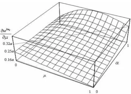
Partial differentiation of (13) with respect to µyields:
∂wit
∂µ =
2t(5 +µ(2−µ))−2a(1−µ(µ+ 2))
(µ(µ+ 2) + 3)2 (B.1)
which is strictly positive whenever µ∈[0.414,1]. If µ∈(0,0.414), (B.1) is only positive when t is high enough relative toa. This, however, is always true within the interval of trade costs consistent with this regime,t∈[tB, tA]. Evaluating (B.1) at the inferior limit
of this interval we have
∂wit ∂µ ¯ ¯ ¯ ¯t=tB = 4a(µ+ 2) (µ(µ+ 1) + 4)(µ(µ+ 2) + 3) >0 which implies that ∂wit
Figure 5: Derivative of wtwI with respect toµ
Implications of the level of union density for wtw1
Partial differentiation of (20) with respect to µyields:
∂wtw1 ∂µ = 4a(4µ−1) +t(11−8µ) + 9t(8a+t(1 + 7µ))/Ψ 8(µ(2µ−1) + 5) + (4µ−1)(4a(µ(1−2µ)−3) +t(µ(4µ−11) + 15) + Ψ 8(µ(2µ−1) + 5) (B.2) which is strictly positive when t ∈ (tE, tD). To prove this, we substitute t in (B.2) by
αtD+(1−α)tE,whereα∈[0,1], and plot the resulting expression in (µ, α)−space (Figure
5). The algebraic proof of this result is here presented for the two extreme cases α = 0 and α= 1.19 ∂wtw1 ∂µ = ( 6a(1+2µ) 24+µ(6µ3+3µ2+22µ+1) 2a(2+µ) (1+µ)(16+µ(3µ−1)) ift=tD ift=tE
Impact of trade liberalisation on wtw1
When µ∈(2
3,1], the wage function wtw1 :
(i) Decreases with trade liberalisation ift∈(t∗, tD)
(ii) Reaches its minimum level whent=t∗
(iii) Increases with trade liberalisation if t∈(tE, t∗).
where,
t∗= 70−151µ+ 50µ2−9µ3+ 3(14−µ(5−µ))
1
2(15−µ(11−4µ))
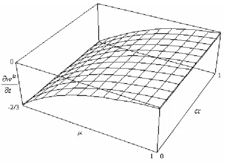
(14−µ(5−µ))(9µ(7µ+ 2) + 335) 8a. Proof proceeds by differentiation of (20) with respect to the level of trade costs:
∂wtw1
∂t =
(8a(9µ−5) +t(335 + 9µ(7µ+ 2)))/Ψ +µ(11−4µ)−15
8(µ(2µ−1) + 5) (B.3) Evaluating (B.4) att={tD, t∗, tE}, we can see that:
∂wtw1 ∂t = 2+µ(5−µ) 6−2µ(1−µ) 0 2−3µ 6(µ+1) ift=tD, and thus >0 if µ∈(2 3,1] ift=t∗ ift=tE, and thus <0 if µ∈(23,1]
When µ∈(0,23], the wage function decreases with trade liberalisation in the full range of trade costs consistent with this regime, t∈[tE, tD].It can be easily checked that:
(i) t∗=tE and ∂wtw1 ∂t |t=tE = 0 (ii)t∗ > tE and ∂wtw1 ∂t |t=tE >0 ifµ= 23 ifµ∈(0,23] In order to prove convexity ofwtw1 int, we compute:
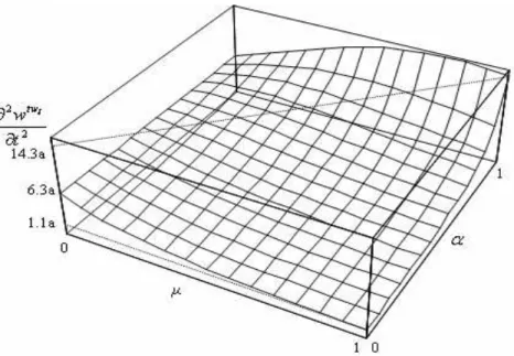
∂2wtw1
∂t2 =
576a2
(64a2+ 16at(5−9µ)−t2(9µ(7µ+ 2) + 335))3/2 (B.4)
This partial derivative is strictly positive whent∈(tE, tD). To prove this, we substitutet
in (B.4) byαtD+(1−α)tE withα∈[0,1], and plot the resulting expression in (µ, α)−space
(Figure 6). The algebraic proof of this result is here presented for the two extreme cases
α= 0 and α= 1.20 ∂2wtw1 ∂µ2 = ( (3µ(µ+1)+8)3 648a(1+µ)3 (µ(3µ−1)+16)3 648a(1+µ)3 ift=tD ift=tE
Figure 6: Second derivative of wtwI with respect tot
C
Extensions to the basic model
C.1 Rent maximising union
For the sake of brevity, we confine our attention to the expressions needed to show that the main findings of the basic model remain qualitatively unchanged. WhenU1 =w(y11+y12),
the outcome of wage bargaining becomes:
wa = aµ2 2(1 +µ2) (C.1) wit = a(5 +µ(2 + 3µ))−4t(1−µ)−Σ 4(1 +µ)2 (C.2) wow = (a+t)µ(1 +µ) 4µ(1 +µ)) + 8 (C.3) wf t = aµ(1 +µ) 4µ(1 +µ)) + 8 (C.4) where Σ =£(a(5 +µ(2 + 3µ))−4t(1−µ))2−8a(1 +µ)2(a(1 +µ2)−2t(1−µ))¤12. In
Figure 7: Derivative ofwit with respect tot tA = µ(1 +µ)(2 +µ) + 2 4(1 +µ2) a (C.5) tB = 4 + 3µ(1 +µ) 8 + 4µ(1 +µ)a (C.6) tD = µ(µ+ 1) + 4 8 + 5µ(1 +µ)a (C.7)
Implications for Propositions 1, 2 and 3
To check whether Proposition 1 remains valid, we compute the partial derivative of (C.2) with respect to t: ∂wit ∂t = µ−1 (µ+ 1)2 µ 1−a(3−µ(2−µ))−4t(1−µ) Σ ¶ (C.8) From (C.8) one can see that ∂w∂tit is strictly negative when t∈(tB, tA) and µ∈(0,1).
To prove this result, we substitutet in (C.8) byαtA+ (1−α)tB withα∈[0,1], and plot the plot the resulting expression in (µ, α)−space (Figure 7).
The algebraic proof of this result is here presented forα={0,1}: ∂wit ∂t = ( 2(µ−1) 3+µ(2+5µ+2µ3) 4(µ−1) 6+µ(8+µ(7+µ(2+µ))) ift=tA ift=tB
We now examine how the assumption of rent maximisation affects Proposition 2. Substi-tuting (C.7) into (C.3) yieldswow|
t=tD = 16+103µ(µµ+1)(µ+1)a,which is strictly higher than (C.1)
if µ∈ (0,0.47). With regard to Proposition 3, by using (C.4) and (C.1) it can be easily checked that wf t> wa ifµ∈(0,0.296).
C.2 Open-shop unions in both countries
When w2 is also the subject of bargaining, we may use (3) to derive the product market
equilibrium expressions taking now into account that w2 ≥0. It is then straightforward
to solve for the steady-state Nash equilibrium wages of both firms (w1 = w2 = w). In
autarky the wage in each firm is set in isolation and therefore it is given by (14). If
t≤ 1
2(a(1 +µ) +wi(1−µ)−2wj) i, j= 1,2;i6=j (C.9) we have theimport threat regime and wages are given by:
wit= a(1 +µ2)−2t(1−µ)
5 +µ2 (C.10)
Substituting either (14) or (C.10) into (C.9) yields
tA= 1 +µ
2 +µ2a (C.11)
Under free trade (t= 0), equilibrium wages are given by:
wf t= µ(1 +µ)
4(2 +µ(1 +µ))a (C.12)
Implications for Propositions 1 and 3
From (C.10) and (C.11) it is clear that Proposition 2 applies as before. Partial differenti-ation of wit with respect tot yields:
∂wit
∂t =−
2(1−µ) 5 +µ2 <0
if µ ∈ (0,1). Comparing (C.12) and (14), one can easily check that wf t > wa if µ ∈
(0,0.333), and hence Proposition 3 remains qualitatively unaltered.
C.3 The outcome of the wage bargain with a strictly positive competi-tive wage
With wc>0 the outcome of the wage bargain for each trade regime is given by:
wa = aµ2 µ2+ 2 (C.13) wit = a(1 +µ2)−2(t+wc)(1−µ) µ(µ+ 2) + 3 (C.14) wow = (a+t+wc)(µ+ 1)µ 2µ(µ+ 1) + 8 (C.15) wtwI = (4a+w c) (µ(2µ−1) + 3)−t(µ(4µ−11) + 15)−∆ 8 (µ(2µ−1) + 5) (C.16) wtwII = µ(µ+ 1)(2a+ 2w c−t) 4 (µ(µ+ 1) + 4) (C.17) where ∆≡[64(a2+wc2 )−16a(9tµ−5t−8wc)−t2(µ(63µ+ 18) + 335)−16t(9µ−
5)wc]12. Furthermore, with a strictly positive competitive wage, there is animport deter-rence regime in the transition between the import threat case and one-way trade. This is given by:
wid= 2(t+wc)−a (C.18)
The locus µmin
Using (C.13)-(C.17) we obtain the expression forµmin under each regime:
µamin = µ 2wc a−wc ¶1 2 (C.19) µitmin = £ 4t2−4(a−2t−5wc)(a−wc)¤12 −2t 2(a−wc) (C.20) µowmin = 1 2 "µ a+ 31wc+t a−wc+t ¶1 2 −1 # (C.21)
µtw1 min = (2a−2wc−t)(a−5t−2wc) + Γ 2(2wc+t−2a) (C.22) µtw2 min = 1 2 "µ 2a+ 62wc−t 2a−2wc−t ¶1 2 −1 # (C.23) where Γ = h (2wc+t−2a)(34at−7a2−31t2+ 78awc−66twc−71wc2i12 . Similarly, we can define a minimum level of trade costs above which the import deterrence wage is above wc:
tidmin= a−wc
2 (C.24)
Proof of Proposition 4
Using (C.19) and (C.23), it can be easily checked that µamin > µf tmin ifwc∈(0,191a).
References
Booth, A. and Chatterji, M. (1995). ‘Union membership and wage bargaining when mem-bership is not compulsory.’, Economic Journal, vol. 105, pp. 345-360.
Brander, J. (1981). ‘Intra-Industry Trade in Identical Commodities.’ Journal of Interna-tional Economics, vol. 11, pp. 1-14.
Corneo, G. (1993). ‘Semi-unionised bargaining with endogenous membership and manage-ment opposition.’, Journal of Economics, vol. 2, pp. 169-188.
Corneo, G. (1995). ‘Social custom, management opposition and trade union membership.’,
European Economic Review, vol. 39, pp. 275-292.
Cramton, P. and Tracy, J. (1998). ‘The use of replacement workers in union contract negotiations: The U.S. experience, 1980-1989’, Journal of Labor Economics, vol. 16, pp. 667-701.
Dempsey, J. (2005). ‘In Europe, Division Among Old and New.’ International Herald Tribune, June 13.
European Commission (2005). ‘The EU Economy 2005 Review’.European Economy, vol. 6, Luxembourg: Office for Official Publications of the EC.
Gramm, C. (1991). ‘Employers decisions to operate during strikes: consequences and policy implications’ in W. Srings, Employee rights in a changing economy: The issue of replacement workers, Washington, D. C.: Economic Policy Institute.
Gramm, C. and Schnell, J. (1994). ‘Some empirical effects of using permanent striker replacements.’, Contemporary Economic Policy, vol. 12, pp. 122-133.
Gunderson, M., Melino, A. (1987). ‘Estimating Strike Effects in a General Model of Prices and Quantities.’,Journal of Labor Economics, vol. 5, pp. 1-19.
Huizinga, H. (1993). ‘International Market Integration and Union Wage Bargaining.’,
Scandinavian Journal of Economics, vol. 95, pp. 249-255.
Lommerud, K.E., Meland, F. and Søgard, L. (2003). ‘Unionised Oligopoly, Trade Liberal-isation and Location Choice.’, Economic Journal, vol. 113, pp. 782-800.
Lommerud, K.E, Meland, F. and Straume, O.R. (2006). ‘Globalisation and Union Oppo-sition to Technological Change.’,Journal of International Economics, vol. 68, pp. 1-23. Naylor, R. (1998). ‘International Trade and Economic Integration When Labour Markets are Generally Unionised.’,European Economic Review, vol. 42, pp. 1251-1267.
Naylor, R. (1999). ‘Union Wage Strategies and International Trade.’, Economic Journal, vol. 109, pp. 102-125.
Naylor, R. and Cripps, M. (1993). ‘An Economic Theory of the Open Shop Trade Union.’,
European Economic Review, vol. 37, pp. 1599-1620.
Naylor, R. and Raaum, O. (1993). ‘The Open Shop Union, Wages, and Management Opposition.’, Oxford Economic Papers, vol. 45, pp. 589-604.
Niblett, R. (2005). ‘Shock Therapy.’ CSIS Euro Focus, vol. 11, June 3.
OECD (2004). ‘Wage-setting Institutions and Outcomes.’ in OECD Employment Outlook 2004 Edition (eds.), Paris: Organisation for Economic Co-operation and Development. OECD (2005a). ‘Trade-Adjustment Costs in OECD Labour Markets: a Mountain or a Molehill?’ in OECD Employment Outlook 2005 Edition (eds.), Paris: OECD.
OECD (2005b). ‘Helping Workers to Navigate in “Globalised” Labour Markets.’, Policy Brief, June, Paris: OECD.