Particle size distribution modeling in the object oriented simulation of gas solid flow

(1)

Particle size distribution modeling in the object oriented

simulation of gas–solid flow

S.J.M. Cartaxo

a

, S.C.S. Rocha

b,∗

, H.B. de Sant’ana

a a_{Federal University of Cear´a, Center of Technology, Department of Chemical Engineering,}

Pici 60455-760, Fortaleza, CE, Brazil

b_{State University of Campinas, Faculty of Chemical Engineering, DTF, Brazil} Received 24 May 2005; received in revised form 12 June 2006; accepted 13 June 2006

Abstract

This work presents an approach to modeling the pneumatic conveying of polydispersed mixtures using the so-called object oriented simulation (OOS) method. Ability to consider a particle size distribution was incorporated into the OOS framework in such a way that it may represent any type of size distribution. Along the model description, several case-studies are accomplished with monodispersed and polydispersed mixtures, which show significant dynamics discrepancies between them, even if the particles mean diameters are the same. This verification is relevant since most of the correlations available to estimate important pneumatic conveying parameters, such as pressure drop and chocking velocity, are based on monodispersed mixtures or use some kind of mean diameter definition.

Keywords: Pneumatic conveying; Polydispersed mixtures; Modeling of gas–solid flow; Particle size distribution

1. Introduction

The understanding of the dynamic phenomena involved in pneumatic conveying of solids requires a fundamental knowl-edge of interaction effects between the continuum and dispersed phases. Probably, the challenge to attain that knowledge is in the great diversity of characteristics that the solid phase may assume, such as density variations, geometry, mechanical properties and size distribution of the carried particles. Although most of real world applications of pneumatic conveying use polydispersed mixture of particles, a wide understanding of the dynamics was not accomplished yet.

Specialized literature brings several correlations to esti-mate relevant project parameters in pneumatic transport sys-tems [1–3]. In spite of being in common use, these corre-lations are restricted to conditions similar to the associated experimental data. Besides, the majority of available exper-imental data is derived from monodispersed mixtures, what makes rather difficult the application to a polydispersed one and

∗_{Corresponding author. Tel.: +55 1937883929; fax: +55 1937883922.}

E-mail addresses:[email protected](S.J.M. Cartaxo),[email protected]

(S.C.S. Rocha),[email protected](H.B. de Sant’ana).

means that any extrapolation will involve risk at least in some extent.

Besides, some studies have disqualified the use of several monodispersed correlations for determining design parameters of systems involving polydispersed mixtures. That is the case of

[4], which obtained unsatisfactory results in the calculation of chocking velocity with all of the correlations evaluated in their study.

The diversity and complexity of physical phenomena verified in particulate two-phase flows demand a rather more fundamen-tal approach, applying fluid dynamic models developed with the goal of providing a deeper understanding of themodus operandi

driving particulate dynamic systems. These fluid dynamic mod-els are nowadays subdivided in two great classes: the continuous eulerians models based on fluid dynamic differential equations

[5–7], and discrete lagrangian models[8,9].

As a variation of the lagrangian concept, it was proposed a discrete object oriented technique [10,11] – named object oriented simulation (OOS) – in which the fluid and particle phases are treated as “real” entities in the model abstraction. By this, it is meant that each particle and fluid elements have its own properties and mechanisms of interaction with the surrounding environment. OOS agglutinates the lagrangian approach and the object oriented paradigm, quite consolidated in disciplines

(2)

Nomenclature

CD drag coefficient dp particle diameter

FC field force upon a particle

FD drag force upon a particle

FR net force upon a particle

g gravity acceleration

mp particle mass r radial position

Rep particle Reynolds number

t time u fluid velocity v particle velocity x particle position Greek letters

µ fluid dynamic viscosity

ρ fluid density

ρp particle density

like electric engineering and computer science. Among the advantages of OOS is the ability of representing any kind of polydispersed mixture with relatively easy, without using a mean diameter. This feature provides the capability of capturing complex phenomena such as clustering and segregation of particles.

Although the OOS approach has potential use to describe a broad range of dynamics systems containing a carrier fluid and particles, as a first application those authors successfully accom-plished the simulation of a turbulent solid–fluid flow through pneumatic conveyor equipment[12].

Appropriate treatment of polydispersed mixtures represents an additional challenge to the study of particulate systems. Continuous models approach this problem subdividing a size distribution in a minimum number of ranges and writing con-servation differential equations for each one of those diameter ranges. This actually means that each size range of particles is treated as a single dynamic phase. On the other hand, discrete models use movement equations to track the path followed by the particles in a more individual basis. Such level of particle individualization makes possible that group interaction phenom-ena are obtained straightly as a result of particle–particle and particles–fluid interactions.

The aim of this work is to present the incorporation of particle size distribution to the OOS method applied for modeling the pneumatic conveying of polydispersed particles.

2. Methodology 2.1. Overview

A very fundamental attribute of the object oriented simula-tion technique is its deterministic and discrete treatment of the particulate phase. Through this perspective, each particle is an

entity in the model’s abstraction. Because of that, one could state that the relevant dynamic phenomena and several interac-tions with the neighborhood are incorporated in each particle model. A direct consequence of this feature is that the simula-tion is performed in a time step transient way, where dynamic state of each entity, being it a particle or fluid element, is updated progressively as the simulated time advances.

For the particles, the displacement is carried out individually by a direct application of three-dimensional transient Newton’s second law(1)along with the velocity definition(2):

dv dt = FR mp , (1) dx dt = v. (2)

The resultant forceFRis a combination of all forces acting on

a single particle, including field and body forces. Disregarding electric and magnetic effects, the resultant force combines the drag forceFD exerted by the fluid and the apparent weight of the particle:

FR= FD+

mp(ρp−ρ)

ρp g. (3)

The OOS allows the calculation of this drag force through any method we find appropriate. In fact, even the solution of the Navier–Stokes equations over the particle external surface may be used. This work was carried out with a more straightforward approach in which the fluid drag force is obtained through a simple drag coefficient definition, given, in this case, by the formulae: CD= 24 Rep 1+Re 0.687 p 6 ; Rep<1000 (4) CD=0,44; Rep≥1000 (5)

where Rep=(ρp|u− v|dp)/(µ). With the drag coefficient

value, we can evaluate the intended drag force from Eq.(6).

FD=CD

πd2_pρ

8 |u− v|(u− v) (6) Particle–particle interactions play an important role in pneu-matic conveying systems. They are responsible for complex phenomena like solids recirculation, clustering, chocking and segregation at some extent. Therefore, it is worth to mention that this work incorporates particle–particle interactions through a collision model used by Kitron et al.[9]. The goal of the colli-sion model is to evaluate the final vectorial velocitiesv₁andv₂

of two particles after they perform a crash, provided the initial velocities,v1andv2, are known. Considering a couple of

collid-ing particles with massesm1andm2, their final velocities after

a collision may be calculated from Eq.(7)bellow:

v_α = vα+(−1)α mR m_␣ {(1+ε)[(v1− v2)· n]n +(1−R)[(v1− v2)· τ]τ}; (7)

(3)

where the index αevaluates to 1 or 2 for the first and sec-ond particles, respectively; mR is the reduced mass given by mR= (m1m2)/(m1+m2);εis the coefficient of restitution, which

ranges from zero to one;ηis the tangential force damping coeffi-cient;nis a unity vector normal to the plane of collision between the particles andτ is the unity vector parallel to that plane of collision.

Rparameter, in Eq.(7), is a function of the approach angle

θ=cos−1((n·(v1 − v2))/(|v1− v2|)), being given by:

R(θ)= ⎧ ⎨ ⎩ 1−η(1+ε)cotanθ; θ∗≤θ≤ π 2 1; 0≤θ < θ∗ , (8)

where θ* is called the cutting angle and is evaluated from

θ*= tan−1η(1 +ε). The functionR(θ) is discontinuous due to the physical fact that the tangential friction force cannot reverse the relative velocities of the particles after a crash.

The transient nature of OOS implies that one may dynami-cally apply modifications to the simulated system, in this case a pneumatic conveyor. In fact, fluid and particles are inserted into the conveying pipe continually, meaning that its properties may be modified anytime as desired, and system will dynamically adapt itself to the new situation.

As particles are injected on a one by one basis at the entrance of the pipe, mathematical “rules” may be created to freely adjust the size of every single particle, in such a way that the whole mixture obeys a specified particle size distribution. This method assures control over any other particle property, e.g. density, sphericity, collision restitution coefficient, etc. These “rules” for artificially simulating a desired polydispersed mixture of gran-ular solids will be derived in a later section.

In order to accomplish the primary goal of this paper, we will set a number of four polydispersed mixtures with the same mean particle size. Particle size distribution of the polydispersed mixtures will be distinct from each other, thus one may compare and analyze the different dynamic behaviors observed.

2.2. Derivation of the size probability distribution

Intending to use the flexibility of setting the size of particles entering the pipe conveyor implies the creation of a rule or pro-cedure to choose the particle diameter value exactly when it is injected into the conveyor so the final mixture follows the pre-defined size distribution function. In order to solve this problem, it is proposed an algorithm based on the definition of a particle population distribution, which designates a curve describing the quantity of particles that belongs to a certain diameter range.

Due to a practical issue, one must consider the standard meth-ods for particle size characterization (e.g. sieves analysis), which provides usually a curve of cumulated mass fraction as a func-tion of particle diameter. Typical informafunc-tion obtained from this curve is the mass fraction of particles having diameter larger than a valued1 and smaller than another valued2. Although

very helpful in a general sense, this is completely useless when developing an algorithm for setting diameter of individual parti-cles. For this case, a curve of cumulated population distribution

is necessary, since it is analogous to a probability distribution function or frequency distribution. Given that the probability distribution function has the ability of defining the chance of an element, randomly chosen inside a population, to pertain to a specific property range[13], we need to convert the measured information (i.e. the particle mass fraction distribution) to the useful one: the particle population distribution.

Consider a size distribution model described by the function

χ=f(D), which, for a given polydispersed mixture, supplies the mass fraction of particles smaller than a diameterD. Therefore, the primary goal is to derive an equation that calculates the popu-lation fraction of particles with diameter smaller thanD, having the general formη=g(D).

Note that a mass fraction differential quantity dχcorresponds to a mass differential quantity dm, through the relation:

dm=mTdχ (9)

wheremTis the total mass of the mixture of particles.

For each mass element dm, there is an associated diameter valueD, which corresponds to a particle of massmp. Then, for

the number of particles dn: dn= dm

mp

. (10)

Considering the previous definition ofχand inserting dχinto Eq.(10)provides:

dn= 6mT ρpπ

f(D)

D3 dD. (11)

In Eq.(11)it was assumed that particle shape permits rea-sonably the definition of a mean diameter, therefore the particle massmpwould be evaluated by:

mp=ρpπD 3

6 (12)

Supposing that a solids mixture has particles with diameters between minimum and maximum valuesDminandDmax,

respec-tively, we can integrate(11)to get the total number of particles

nTas: nT= 6mT ρpπ Dmax Dmin f(D) D3 dD. (13)

The number of particlesnwith diameter larger thanDminand

smaller than an arbitrary valueDmay be calculated from:

n=6mT ρpπ D Dmin f(D) D3 dD. (14)

And, for the fraction of particle population, η, within the range (Dmin,D): η(D)= D Dmin(f(D)/D 3_{) d}_D Dmax Dmin (f ₍_D₎_/D3_{) d}_D. (15)

Eq.(15)is the desired cumulated probability distribution of particles population, or, shortly, population fraction distribu-tion, which calculates the fraction of particles having diameter

(4)

Fig. 1. Typical population fraction distribution for a polydispersed mixture.

smaller than a value D. Therefore, fraction of particles with diameter within the range (D1, D2) may be evaluated from η(D2)−η(D1).

The population fraction distribution function allows the con-struction of a diagram describing the size profile for a particular sample of particles. Consequently, application of Eq.(15)to the mass fraction distribution obtained from standard sieves analy-sis results in a population fraction distribution curve, which is typically illustrated inFig. 1.

With the aid ofFig. 1, the application of Eq.(15)to generate a particle size distribution is explained as follows. Since the curve inFig. 1is based on the particles population, i.e. the number of particles within a size range, we may subdivide the vertical axis (fraction population) into even intervals of same probability. Each one of these intervals corresponds to a diameter range on the abscissa; therefore the algorithm consists in introducing the same number of particles in each diameter range. The insertion of the same quantity of particles in the intervals of equal population fraction reproduces the original size distribution.

One should notice that the use of Eq.(15)is subjected to a number of numerical issues. Firstly, it requires the definition of a non-zero minimum particle diameter, other way the integral would overflow. Additionally, round off errors may be signifi-cant if lower limit of the integral is sufficiently small. In order to overcome these numerical problems, we define a physically acceptable minimum diameter bellow which the population frac-tion is zero. By doing this, the Simpson’s method for numerical integration may be successfully applied to derive the population fraction from Eq.(15).

2.3. Particle size distributions

In order to analyze the effect of size distribution on the dynamic behavior of the conveyed mixtures, four polydispersed mixtures with distinct particle size profiles were selected. Intend-ing to assure a base for comparison, all of the polydispersed mixtures studied in this work are a blend of glass particles with density of 2470 kg/m3, diameter in the range of 0.5 mm

Table 1

Terminal velocity and mass fraction for each particle size used to compose the several polydispersed mixtures

D(mm) Vt (m/s) Mass fraction A (%) B (%) C (%) D (%) 0.5 3.9 0 0 0 0 1.0 7.2 61.4 2.9 36.3 24.7 1.5 10.1 0.3 44.2 3.1 25.0 2.0 12.0 1.0 52.9 46.6 25.0 2.5 13.5 1.4 0 2.6 25.2 3.0 14.8 35.9 0 11.4 0

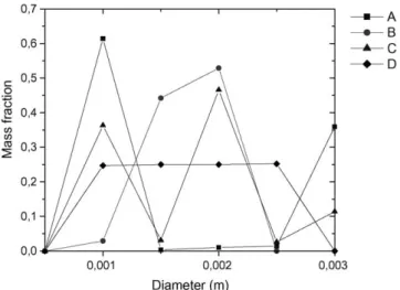
Fig. 2. Cumulated mass distribution for the studied solids mixtures.

to 3.0 mm and have the same average particle diameter of about 1.5 mm.Table 1shows the terminal velocity of all particle types and their concentration in each of the blends. Single particle terminal velocities are evaluated for air with density of 1 kg/m3 and cinematic viscosity equal to 1.8E−5 Pa s.

Fig. 2presents the cumulated mass fraction as function of the particle diameter; much like one would obtain from standard sieves classification of the solids mixture. A baseline is

(5)

lished by curve E, which stands for a monodispersed sample of particles with 1.5 mm diameter.

To achieve more insight about the mixtures content, curves inFig. 2may be converted into mass distribution ones, as shown inFig. 3. From those curves, it is seen that mixture A is mainly composed of smaller and greater particles having no particles with medium diameter. Mixture B is also a binary one, but has a narrow size distribution. Mixture C is ternary and has a broad range of particles sizes, being less concentrated in the larger particles. At last, mixture D is a broad range equal combination of all sizes, except for 3.0 mm.

3. Results

Computational simulations were performed for all polydis-persed mixtures in a pipe conveyor with 0.1 m diameter and 3 m height. Carrier fluid is air with density of 1 kg/m3and cinematic viscosity equal to 1.8E−5 Pa s.

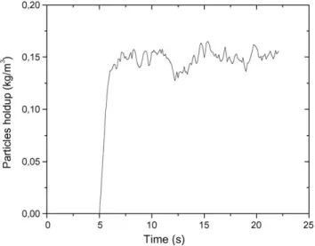
As a standard procedure, an injection rate of 3000 particles per second was applied after fluid flow steady state. Then, subse-quent to particles injection, simulations were carried out[10,11]

till holdup of solids achieved steady state also, as one may see inFig. 4. Only after steady state was achieved properties values were evaluated and the results were collected and analyzed.

Intending to avoid particles precipitation for reasons other than solids dispersion and recycling, average fluid velocity was adjusted to about 20 m/s, so being above the highest terminal velocity corresponding to particles of 3.0 mm diameter (see

Table 1). This way, it is quite guaranteed that the fluid phase is able to drag all particles, except for the particles that are in very near wall locations.

Fig. 5brings the cumulated mass fraction for the mixture A at different places of the conveyor. “Top” curve regards to particle size distribution of particles being actually conveyed, so they exit through the top of the pipe, while “Pipe” line refers to size distribution of particles inside the conveyor. “Bottom” represents the particles size distribution for non-transported particles, i.e. these particles fall down to the pipe bottom and are outcome of

Fig. 4. Typical time profile of particles holdup inside the pipe.

Fig. 5. Cumulated mass distribution for mixture “A” at different places of the conveyor.

solids dispersion caused mainly by inter-particles collisions. For easier comparison, it is also shown the initial size distribution for the particles entering the pipe (“Entrance”).

From those size distributions inFig. 5, one can observe the solids segregation phenomenon, by which composition of con-veyed solids becomes distinct from the original mixture. Indeed, solids exiting at the top of pipe are richer in smaller particles of 1.0 mm diameter. This observation agrees with physical expec-tation, since heavier particles have higher precipitation trend. In contrast, if compared with the original size distribution, size profile inside the pipe is shifted to larger diameters; whereas the bottom size distribution reveals that quite few small particles fall down.

One can reason more clearly the dynamic behavior observed for mixture A if the non-cumulated mass distribution inFig. 3is considered. That curve reveals that solids blend contains mainly two kinds of particles with significantly different diameters. Therefore, it is naturally expected that these two dynamic phases separate with relatively easy with heavier particles going to the conveyor bottom. Actually, it may be remarked that 3.0 mm particles effectively constitutes a single dynamic phase, which distributes between the top and the bottom regions, being trans-ported only partially by the fluid.

The inspection ofFig. 3reveals a major concern we must be aware when designing or analyzing pneumatic conveying sys-tems for a multi-sized blend of solids. Commonly, practitioners and researchers adopt a mean particle diameter to perform the equipment sizing, however the mixture A behavior indicates that a polydispersed mixture may originate a few dynamic phases which have different sizes distributions, affecting therefore the rate of effectively conveyed particles and other important design parameters such as choking velocity and pressure drop.

Mixture B raises a distinct picture. As seen inFig. 6, cumu-lated mass distribution curves for these solids blend are close among the several conveyor locations, indicating lesser segre-gation effect than that verified for mixture A. Profiles for top, pipe and entrance locations are nearly coincident. This allows inferring that solids composition inside the pipe is almost equal to the one of transported particles.

(6)

Fig. 6. Cumulated mass distribution for mixture “B” at different places of the conveyor.

Referring toFig. 3, it is immediately verified that mixture B corresponds to a narrow size distribution, containing particles with near diameter values. Therefore the verified behavior in

Fig. 6 indicates that polydispersed mixtures with narrow size distribution may behave much like a monodispersed system. Hence, the direct conclusion is that design parameters for this type of mixtures may be estimated through correlations based on data measured for monodispersed particles with relatively safety.

Segregation is also prominent for mixture C, which is com-posed of three particles types with very distinct diameters. Accordingly, a significant effect of segregation may be seen in

Fig. 7. The size distributions for the entrance and top regions are almost coincident; however there is a large gap between the pipe and the bottom curves, meaning that the mixture of solids leaving the bottom of the conveyor is richer in particles with larger diameters, mostly 3.0 mm.

In its turn, the quaternary mixture represented by the blend D implies less segregation than mixture C, as seen inFig. 8. For this polydispersed mixture, the particles sizes are equally distributed corresponding to a flat particle size distribution (seeFig. 3). As

Fig. 7. Cumulated mass distribution for mixture “C” at different places of the conveyor.

Fig. 8. Cumulated mass distribution for mixture “D” at different places of the conveyor.

for the other blends, the top curve matches the particles size distribution at the entrance. The bottom curve clearly deviates from the other ones, exhibiting greater concentration of larger particles, especially with diameters above 2.0 mm.

4. Conclusions

A method to incorporate the capability of simulating the dynamic behavior of polydispersed mixtures of particles into the object oriented simulation framework[10]was presented. The proposed approach is based on the concept of size probabil-ity distribution, which has led to the definition of the population fraction distribution curve, used in the algorithm of generat-ing the particles diameters. The population fraction distribution curve results from the conversion of standard information on par-ticle size characterization, as obtained with an ordinary sieves analysis.

In order to demonstrate the feasibility of the developed approach, four case-studies involving polydispersed mixtures with the same mean particle size were performed. Simula-tions were run for each case study and results have shown noticeably the segregation phenomenon at different levels of severity, according to the shape of the particle size distri-bution. Mixtures with a broad size distribution exhibit more segregation than blends with a narrower one. As a conse-quence, polydispersed mixtures with sufficiently narrow par-ticle size distribution may be treated like a monodispersed system.

On the other hand, the level of segregation verified with some polydispersed mixtures suggests that practitioners and researchers should apply caution when relying on correlations, based on monodispersed experimental data, for designing or analyzing polydispersed transport systems.

Acknowledgements

The authors would like to acknowledge and thank the finan-cial support of: Fundo de Desenvolvimento Cient´ıfico e Tec-nol´ogico do Nordeste (FUNDECI) do Banco do Nordeste S.A.

(7)

and CNPq (Brazilian National Research Council), for the devel-opment of this research work.

References

[1] F.A. Zenz, Two-phase fluid–solid flow, Ind. Eng. Chem. 41 (1949) 2801–2806.

[2] L.S. Leung, R.J. Wiles, A quantitative design procedure for vertical pneu-matic conveying systems, Ind. Eng. Chem. Process. Des. Develop. 15 (1976) 552–562.

[3] T.M. Knowlton, D.M. Bachovchin, Fluidization Technology, vol. 2, Hemi-sphere, Washington, 1976, pp. 252–282.

[4] C.L. Briens, M.A. Bergougnou, New model to calculate the choking veloc-ity of monosize and multisize solids in vertical pneumatic transport lines, Can. J. Chem. Eng. 64 (1986) 196–204.

[5] S.L. Soo, Fluid Dynamics of Multiphase Systems, Blaisdell Publishing Company, 1967.

[6] R. Jackson, Fluid Mechanical Theory in Fluidization, Academic Press, New York, 1971.

[7] M. Ishii, Thermo-Fluid Dynamic Theory of Two Phase Flow, Eyrolles, 1975.

[8] C.T. Crowe, M.P. Sharma, D.E. Stock, The particle-source-in-cell (PSI-cell) model for gas-droplet flows, ASME, J. Fluids Eng. 99 (1977) 325– 332.

[9] A. Kitron, T. Elperin, A. Tamir, Monte Carlo simulation of gas–solid sus-pension flows in impinging-reactors, Int. J. Multiphase Flow 16 (1) (1990) 1–17.

[10] S.J.M. Cartaxo, S.C.S. Rocha, Object oriented simulation of the fluid-dynamics of gas–solid Flow, Powder Technol. 117 (3) (2001) 177– 188.

[11] S.J.M. Cartaxo, Object-oriented simulation of pneumatic conveying, Ph.D. thesis, State University of Campinas, Campinas, SP, Brazil, 2000.

[12] S.J.M. Cartaxo, S.C.S. Rocha, Object-oriented simulation of pneumatic conveying—application to a turbulent flow, Braz. J. Chem. Eng. 16 (4) (1999) 329–337.

[13] G.E.P. Box, W.G. Hunter, J.S. Hunter, Statistics for Experimenters, John Wiley & Sons, 1978.