Cloud-based video analytics using convolutional neural networks.

Cloud-based Video Analytics using Convolutional

Neural Networks

Muhammad Usman Yaseen

1

∗

| Ashiq Anjum

1

∗

|

Mohsen Farid

1

∗

| Nick Antonopoulos

1

∗

Mathematics, University of Derby, Derby, Derbyshire, DE22 1GB, UK

Correspondence

Muhammad Usman Yaseen, Department of Computing and Mathematics, University of Derby, Derby, Derbyshire, DE22 1GB, UK Email: [email protected]

Funding information

Object classification is a vital part of any video analytics

sys-tem which could aid in complex applications such as object

monitoring and management. Traditional video analytics

systems work on shallow networks and are unable to

har-ness the power of distributed processing for training and

inference. We propose a cloud-based video analytics system

based on an optimally tuned convolutional neural network

to classify objects from video streams. The tuning of

con-volutional neural network is empowered by in-memory

dis-tributed computing. The object classification is performed

by comparing the target object with the pre-stored trained

patterns, generating a set of matching scores. The

match-ing scores greater than an empirically determined threshold

reveal the classification of the target object. The proposed

system proved to be robust to classification errors with an

accuracy and precision of 97% and 96% respectively and can

be used as a general-purpose video analytics system.

Cloud Computing, Convolutional Neural Networks, Deep Learning, Hyperparameter Tuning, Video Analytics

Abbreviations:CNN, Convolutional Neural Networks; LR, Learning Rate; SGD, Stochastic Gradient Descent. ∗_{Equally contributing authors.}

1

|

INTRODUCTION

Object classification is an important part of any video analytics system. It has its applications in police, airports, hospitals and a number of other organizations. It helps to classify objects by matching the provided sample with the already stored patterns in a database. Traditional video analytics systems performing object classification uses shallow networks. In contrast, we propose a cloud-based system that learns features automatically from pixels for the classification task. It uses a convolutional neural network for classification of objects. The proposed system employs detection and extraction phases to detect and extract desired objects from decoded video frames.

We have used the concept of adaptive frame sampling during the decoding and detection phase. In the adaptive frame sampling, only those video frames are retained which contained the objects in them. All the video frames which do not possess anything are discarded. In a video stream, the consecutive video frames are more likely to contain the same object with the same pose and lightning conditions. Due to constraints on motion, no change can occur in such a short interval of time. For consecutive video frames we took 5 frames out of 25 per second as the fps is set to 25. So we have a frame sampling rate of 5. The frame sampling helps in discarding redundant frames and leads to less data transfer to the cloud, which in turn reduces the training time.

The normalization is performed in order to change the dynamic range of pixel intensity values. The objective is to achieve consistency in the dynamic range of video frames for the training of convolutional neural network. We have normalized the values of the video frames to range [0, 1]. The dynamic range of video frames to [0, 1] is better than [0,255] for the training of convolutional neural network because latter can cause numerical issues during the learning of first layer weights in CNNs [10]. Also, we have performed the training by using gradient descent and used the same learning rate across all weights, so the normalization helped to have the similar distribution across the network. The normalization does not had any negative effects on the extracted objects as the extracted objects do not possess extreme values and can be fully represented by the pixels in the constrained range of [0, 1].

We harnessed the power of an in-memory cloud for parallel model training. The trained parameters from each partial model on each node are averaged using parameter averaging. This procedure reduces the overall training time which would have been very high in case of training the model as a whole. The trained classifier from cloud is saved locally and is further used to perform object classification.

A sample of the target object which is to be classified in the video streams is passed through the trained classifier. The trained classifier returns the probabilities or matching scores of the possible labels for the object. Only the probabilities of the possible labels are returned but not the labels themselves. The labels of all the objects present in all the video streams were pre-stored in the database beforehand. The object with the highest probability (above an empirically determined threshold) indicates the classification of the object. The probabilities closer to 1 depict a closer match of the object and the probabilities close to 0 depict the unavailability of the object in the video streams.

The contributions of this paper are the following: Firstly, a system to classify objects in video streams is presented. Secondly, we perform parallel model training on an in-memory distributed cluster. Thirdly, we propose an optimally tuned convolutional neural network model that best suits for a general purpose video analytics system. This paper is an extension of our work published in [31].

The remaining sections are organized as: Section II reviews the related work. Section III presents the proposed approach. Section IV presents the architecture and implementation details. Experimental setup and results are described in Sections V and VI respectively. Section VII concludes the paper.

2

|

RELATED WORK

Video analytics is an active area of research from the recent past. Researchers have exploited the use of color and texture to perform object classification. [20] proposed an ensemble of different approaches and combined them on color spaces. They extracted both the color and texture features from the images and made a comparison of them on the basis of distance measures. Other studies [12] [6] [34] [17] also exploited the use of color features but all these approaches built upon the color and texture properties fail in the case of strong illumination conditions. Some approaches [16] made the use of local features and generated a set of key-points to produce the signature of target object. But the accuracy of these approaches is highly dependent on the performance of key-point detector.

A number of studies [27] [30] [29] [9] worked on multi-modal features. They used hidden markov models [8], guassian density functions [22] and local pattern features [2] [32] in their system. [5] used a probabilistic fusion scheme to fuse the features from different modalities and then performed the classification. [7] proposed a rank-level fusion approach to fuse the features from different modalities. Then a majority voting rule was applied to perform decision. However, all these approaches need to have a good compromise between computational cost and performance as the use of multi-modal features generate large feature vectors.

The deep learning based approaches can overcome the weaknesses of hand crafted features as they have the ability to learn features automatically from the input data. Deep learning based algorithms such as convolutional neural networks can learn features directly from the pixels of images or video frames. Convolutional neural network performed quite well recently. Several approaches [11][23] employed convolutional neural networks to perform large scale object classification. Similarly [13] used convolutional neural network to perform age and gender classification.

Few recent studies have made the use of deep learning based approaches for video analytics. [14] proposed a filter pairing neural network. They jointly optimized all the components of the system to handle geometric and photometric transforms and achieved good results on their self-generated dataset. Similarly [33] proposed a siamese deep neural network to learn a similarity metric from pixels in a unified framework.In another study [3], a deep convolutional architecture was proposed to simultaneously learn features and corresponding similarity metric. However, they input a pair of images and tried to find a similarity value to indicate whether the two images belong to same object or not. They performed more of a verification task than classification of objects.

Most of the existing video analytics systems lack distributed processing in them. Due to this reason, these systems train on small datasets and severely suffers from accuracy and performance degradations. We propose an optimally tuned convolutional neural network based video analytics system in this work. The system is empowered by an in-memory distributed training mechanism. The proposed system can be used as a general purpose video analytics system.

3

|

VIDEO ANALYTICS APPROACH

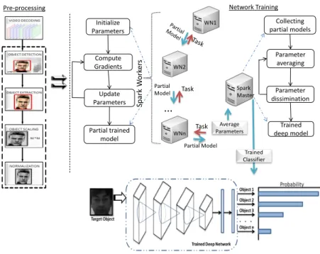
In this section, we present the approach behind the proposed video analytics system.The mathematical modeling of the system helps to tune the hyper-parameters of the system by observing the effects of different hyper-parameter values on the overall performance of the system. Figure 1 shows the approach of our proposed video analytics system. The proposed system first decodes the input video stream. The decoded video frames dataset “X" can be repre-sented as;

...

Model Spark_Master WN1 WN2 WNn Collecting partial models Parameter averaging Parameter dissimination Trained deep model Initialize Parameters Compute Gradients Update Parameters Partial trained model Task Partial Model

Pre-processing Network Training

Trained Classifier

F I G U R E 1 Architecture of the Proposed System

Here, “x₁,x₂, . . .xn" are frames in the dataset.

The decoded frames then go through the detection phase which associates a bounding box around the area of detection. A labeled frame in our system is represented by (x; c) where0_x0_{represents the frame and‘c}0_represents

the ground truth. The associated bounding box is represented by;

R(x0,y0xn,yn) (2)

Adaptive frame sampling is used during the decoding and detection steps where only those video frames are retained which contain objects in them. All the video frames which do not possess any object are discarded. In the video stream, the consecutive video frames are more likely to contain the same object with the same pose and lightning conditions. Due to constraints on motion, no change can occur in such a short interval of time. The frame filtering and sampling helps in discarding redundant frames and leads to reduced data for transmission to the cloud data center, which in turn reduces the training time. For consecutive video frames we select only 5 frames per second. The total number of frames generated per second is 25 as the frame per second rate is set to 25. So we have a frame sampling rate of 5 in the proposed system.

The extracted objects are scaled at 150*150 pixels. A normalization having a range of [0,1] instead of [0,255] is also performed as the latter can cause numerical issues during the learning of first layer weights in CNNs.

Figure 2 depicts the procedure of training the deep learning model. All the variables are first initialized and the datasets for training the model are loaded from the storage. We have defined a record reader which iterates over the records. The normalizer is then initialized to normalize the dataset. After determining the labels for the

Initialize all variables to use Load the training and testing data Determine image labels Initialize reader to read the records Initialize the normalizer Build the deep

network Train the network Evaluate the model Generate evaluation statistics

F I G U R E 2 Model Training Process

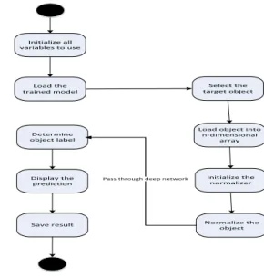
Initialize all variables to use Load the trained model Determine object label Initialize the normalizer

Pass through deep network

Select the target object

Load object into n-dimensional array Normalize the object Display the prediction Save result F I G U R E 3 Classification Process

extracted objects from the video frames, the deep neural network is built. All the layers of the deep network are defined and initialized with their respective parameters.

There are two convolutional layers in the network. The first convolutional layer has 50 kernels in it with a mension and stride of 150 x 150 x 1 and 1 x 1 respectively. Stride controls how depth columns around the spatial di-mensions are assigned. The next layer has 100 kernles in it with a dimension and stride of 5 x 5 and 1 x 1 respectively. These layers constitute nonZeroBias. Each layer constitutes ’RMSPROP’ updater and ’relu’ as an activation function. The kernel size of both the convolutional layers is [5,5]. There are two max pooling layers which are followed by each convolutional layer in the network. There is one output layer which is followed by one dense layer. The kernels and neurons of the subsequent layers has a connection with the previous layers. A momentum of 0.9 is selected. The dense and output layers have a layer size of 500 and 34 respectively. Each layer constitutes ’RMSPROP’ updater. The value of learning rate is selected to be 0.0001. It has been selected after a number of experiments.

The layers of the CNN are represented as;

C onvk,l =g(xk,l∗Wk,l +Bk,l) (3)

Subk,l =g(↓xk,l∗wk,l+bk,l) (4)

Table 1 depicts the basic configuration parameters of convolutional layers. The activation function is represented as;

h=max(₀,a)w her e a=W x+b (5)

The Local Response Normalization is used for generalization. The Local Response Normalization simulates the behavior of actual neurons and generates a competition amongst neuron outputs. The pooling layer performs

sam-TA B L E 1 Layers Configuration Layer Info. Convolutional 1 Convolutional 2 Layer Size 50 100

Kernel Size [5,5] [5,5] Updater RMSPROP RMSPROP Weight Init. XAVIER XAVIER Stride [1,1] [1,1] Activation ReLU ReLU

ple based discretization or downsampling of an input representation (feature maps from convolutional layer in our case). It reduces the dimensionality of the features. L2 regularization is used to avoid over-fitting. L2 regulariza-tion penalizes the squared magnitude of parameters. It penalizes peaky weight vectors heavily and prefers diffuse weight vectors. Training the model on large amount of data on multiple nodes of a cluster also helped to prevent the problem of under-fitting. L2 regularization adds

λ₂Õ

i

θ_i2 (6)

This is added for every weight in the network directly in the objective. In this equationλrepresents the strength of the regularization.

The bias and weight deltas which are updated in backpropagation are given as;

4Wt,k =LR F Õ i=1 (xi∗Dhi)+m4W(t−1,k) (7) 4Bt,k =LR F Õ i=1 D_ih+m4B(t−1,k) (8)

These weight and bias deltas are used to have a better estimate of the gradient during training. The loss function which we try to minimize during training is represented as;

L(x)=LR Õ

xi−>X

Õ

xi−>Ti

l(i,xiT) (9)

The loss function is the measure of the difference between the actual outcome and the prediction of the network. The stochastic gradient descent which reduces the loss function is represented as;

Wt+1=Wt−α δL(θt) (10)

Vt+1=ρvt−α δL(θt) (11)

Wt+1=Wt+Vt+1 (12)

The softmax layer is represented as;

T R(i,xiT)=M(ei,f(xiT)) (13)

The trained classifier is then used to perform object classification for our video analytics system as shown in Figure 3. The target object which is to be classified is passed through the trained network. The target object passes through the same normalization procedure before passing through the deep network. The trained model then gen-erates a set of probabilities against the target object. The highest probability determines the label of the target object. The number of object classes to be determined by the system are represented as;

Y(i)= 1,2, . . .K (14)

where 1,2, ...K represents the total number of possible classes. Our hypothesis function for the classification task is given by;

hθ(x)= 1/(1 +exp(−θTx)) (15)

whereθrepresents the trained model parameters that minimize the cost function. The hypothesis function estimates the probability P(y = k | x) for each value ofK= 1,2, . . .K. The system then estimates the probability of the class label and produces an output vector with ’K’ estimated probabilities. The hypothesis function takes the form;

hθ(x)=                    P(y= 1|x;θ) P(y= 2|x;θ) · · · P(y=K|x;θ) (16)

4

|

SYSTEM IMPLEMENTATION

A distributed cloud infrastructure [19] [21] has been used to train the proposed video analytics system. Distributed infrastructures have been used actively in the past [26] [25] [15] to improve the performance of a compute intensive system. The proposed system is also compute intensive and necessitates parallel model training. The training of the model is parallelized by adopting Apache Spark [24] computing framework. Each node in the spark cluster trains a partial model. Iterative parameter averaging is then used to combine the partial models in a central model.

The master node of the spark cluster loads initial configurations. Each node in the cluster performs partial model training on subsets of data. The workers train partial models and their results are averaged through parameter averaging.

Algorithm 1Distributed Training Input:

Input Dataset X =x₁,x₂, . . .,xn, 150 x 150 image size

Network Configurations no. of workers, averaging frequency, minibatchs etc.

Initial Model Parameters momentum/rmsprop/adagrad etc.

Data Split R

Output:

result: Trained Network at Master TR(x) whileData Splits r: 1→Rdo

whileEach Split of Training Data x: 1→Xdo

Distribute network configurations and model parameters to workers Train each model on the worker on its own split

Calculate weight and bias deltas on each worker

4Wt,k=LRÍF i=1(xi∗D_ih)+m4W(t−1,k) 4Bt,k =LRÍF i=1D h i +m4B(t−1,k) Compute error yx−a

Back propagate and update network weights on each worker Wt+1=Wt−α δL(θt)

Average the results from each worker and return the results back to master end

end

In parameter averaging, the network parameters are first initialized depending upon the configuration of the model. The current parameters (a duplicate copy) is transferred to each worker node in the cluster. Each worker node then trains a partial model on a subset of data assigned to it. At the master node, the global parameters are set to average the parameters provided by each worker node as explained in Algorithm 1. This process continues for the whole training dataset.

The subsets of data are then transformed into mini-batches. These mini-batches are serialized with the help of kryo serialization library. The Kryo serialization is much more efficient than java’s own serialization library [18]. The parameter averaging rate is an important parameter to be controlled. A misconfiguration of this parameter can lead to an overhead in initialization. The overhead can also be caused in network communication. The misconfiguration of parameter averaging rate can also degrade performance as the parameters will deviate extensively. We have selected a frequency of 16 mini-batches as it provided the optimal performance in our case.

The data repartitioning strategy is another important parameter. If it is configured properly, it helps to utilize all cluster resources efficiently. We have selected this repartitioning factor on the basis of experimentations to ensure balanced partitions. The iterative map-reduce framework has been used in the proposed system. It executes multiple passes of map-reduce as opposed to simple map-reduce. As the convolutional neural network based systems are are highly iterative so the single pass of map-reduce does not performs quite well. Therefore, iterative map-reduce is a good candidate for such systems.

The configuration of locality in spark is performed according to the computational demands of the algorithm. As the deep learning algorithm which is being executed on spark has high computation demands, it poses high computation per input mini-batch. We have executed one task on each executor; therefore it is much appropriate to transfer the data

Algorithm 2Training of Convolutional Neural Network Input:

Input Dataset x1,x2, . . .,xn, 192 x 168 image size

Output Target Label T 1-in-k vectorsy₁,y₂, . . .,yt

Number of back-propagation epochs R

Number of convolution masks J

Activation function of convolution g(.)

Output:

result: Trained Network TR(x)

whileepoch r: 1→Rdo

whileTraining image number x: 1→_Xdo

Compute J hidden activation matricesz₁,z₂, ...,zj g(xk,l+wk,l+Bk,l) Downsample matricesz1,z2, ...,zjby a factor of 2 g(↓2xk,l+wk,l+bk,l) Calculate weight and bias deltas

4Wt,k=LRÍF i=1(xi∗D_ih)+m4W(t−1,k) 4Bt,k =LRÍF i=1D h i +m4B(t−1,k)

Calculate softmax activation vector ’a’ l(i,xiT)=M(ei,f(xiT))

Compute error yx−a

Back propagate and update network weights Wt+1=Wt−α δL(θt) end

end

Algorithm 3Object Classification Input:

Input Target Object x, 192 x 168 size

Output Target Label T 1-in-k vectorsy1,y2, . . .,yt

Number of Trained Patterns R

Similarity Function f(.)

Output:

result: Classification Labels fco ⇐F ul l y C onnect ed r esul t⇐S of t max(fco) whileTraining vector x: 1→Rdo

Load the trained classifier TR(x)

Apply pre-processing steps on target object’s sample Pass the sample through the trained network

Calculate softmax activation vector ’a’ l(i,xiT)=M(ei,f(xiT))

Compute similarity index yx−a

Generate the set of possible probabilities i end

Input Dataset

Feature Extraction

Classification

Convolution

Max Pooling

Convolution

Max Pooling

Dense

Pre-processed Data

Output

F I G U R E 4 Architecture of Convolutional Neural Network

to a free executor instantly as an executor gets free. It will not be a good setting to wait for a free executor that has local access to the data (default configuration of spark). Transferring the data to a free executor which does not have a local access to data will require the data to be copied across the network, but it allows maximum cluster utilization for our proposed algorithm.

The implementation phase initiates by decoding the video streams into video frames. An open-source library named as Nd4j [1] is used to store the extracted objects from individual frames. A dataset iterator is created which iterates over the dataset objects present in the memory. The dataset objects contain features and labels for the video frames. The training process for CNN is explained in Algorithm 2. A value of 0.0001 is selected for the learning rate on the basis of experimentation. The higher values caused divergence of the network model away from the error minimum. On the other hand, a small value caused slow convergence on an error minimum.

A sample of the target object which is to be classified in the video streams is passed through the trained classifier after training. The trained classifier returns the probabilities or matching scores of the possible labels for the object as explained in Algorithm 3 . The object with the highest probability (above an empirically determined threshold) indicates the classification of the object.

5

|

EXPERIMENTAL SETUP

We present the experimental setup used to evaluate the proposed system in this section. A private cloud has been used to configure in-memory computing based spark cluster. Eight nodes in the cloud are configured to run spark framework. A ubuntu version of 15.04 is installed on each cloud node. Each node has a storage of 100GB, 4vCPUs and 16GB memory.

Most of the video dataset used in the proposed system is self generated. The video streams recorded for the experiments are relatively simple (captured under controlled environmental conditions with faces posing towards a camera) as shown in Figure 5. The extracted objects from the video frames are labeled manually. A directory struc-ture is maintained which contains the frames from the same subject in their respective directories. A number of video streams are captured containing different subjects comprising of almost 100 GB in size. All the subjects ap-pearing in the video streams are mostly facing towards the video camera. Some video streams also contain the rear, side and front poses of the subjects. However, the subjects are not occluded as occlusion has not been considered

F I G U R E 5 Example Faces from Self-generated Dataset

F I G U R E 6 Example Faces from Yale Dataset

F I G U R E 7 Example Faces from BioID Dataset

in this work. The self-generated video dataset also does not posses illumination or other challenges. The duration of each of the video stream is almost 120 seconds.

The video streams are decoded to produce video frames containing side pose, front pose and rear pose of per-sons. The total number of decoded video frames is directly proportional to the duration of video stream being an-alyzed. For a video stream of 120 seconds length, 3000 video frames are generated. All of these video frames are stored as .PNG files. Some publicly available datasets such as BioID [4] and Yale [28] have also been made part of the dataset. The Yale face database has been created to mimic the real world situations. Exceptional importance has been given to the illumination effects which occurs mostly in real life scenarios. The database consists of a va-riety of human faces with diverse facial expressions, poses and illumination effects as shown in Figure 6. There are 34 subjects, each with 60 samples for training and testing. The images are gray scaled and each subject in each image demonstrates variations in illumination conditions (left-right, center-right, rightright) and facial expressions (normal, sad, happy, sleepy).

The BioID Face Database on the other hand also has a diversity of face sizes, background conditions and illu-mination effects. The database contains gray level images captured under varying conditions. For testing purposes, the images are artificially blurred by using a Gaussian blur mask with various sigma values (0, 0.25· · ·). Figure 7 shows some example images from the BioID Face Database.

The network is built upon a total of five layers. There are two convolutional layers in the network with 50 and 100 kernels respectively and constitutes nonZeroBias as shown in Figure 4 . Each layer constitutes ’RMSPROP’ updater and ’relu’ as an activation function. The kernel size of both the convolutional layers is [5,5]. There are two max pooling layers which are followed by each convolutional layer in the network. There is one output layer which is followed by one dense layer. The ReLU non-linearity layer follows all the layers and a momentum of 0.9 is selected.

The dense and output layers have a layer size of 500 and 34 respectively. Each layer constitutes ’RMSPROP’ updater. The dense layer has ’relu’ as an activation function and the output layer has softmax function for classification. The kernels of the following layers are connected to the kernels of the preceding layers. All the neurons in the dense layer are connected to the neurons of the preceding layer. More detailed specifications of these layers are listed in Table 2.

TA B L E 2 Configuration Parameters

Spark Configuration Model Configuration Parameters Values Parameters Values

spark.worker.cores 1 Number of Layers 5

spark.worker.instances 1 nonZeroBias 1

spark.eventLog.enabled TRUE DropOut 0.5

spark.scheduler.mode FIFO OptimizationAlgo SGD

spark.serializer KRYO Activation RELU

spark.rpc.message.maxSize 250 Regularization L2

spark.locality.wait 0 Momentum 0.9

Averaging Frequency 1 Seed 42

Batchsize per Worker 12 Learning Rate 0.0001

Model Score vs. Iteration

MODE L S COR E

ITERATIONS

6

|

RESULTS AND DISCUSSION

In this section, we first describe the performance of the system during training and visualize the performance graphs by tuning the selected parameters. The trained classifier is then evaluated and its performance is measured by the confusion matrix. It is then used in the proposed video analytics system. The scalability of the system is discussed at the end of this section.

Classifier Training Parameters:

The loss function value i.e.L(x)=LRÍ

xi−>X

Í

xi−>Til(i,xiT)at various iterations of the current minibatch is shown in Figure 8 . It can be observed in the figure that loss narrows down after each iteration over time. It depicts that the learning rate is set properly. The values of the learning rate are varied to 1e-2, 1e-4 and 1e-6. It was observed

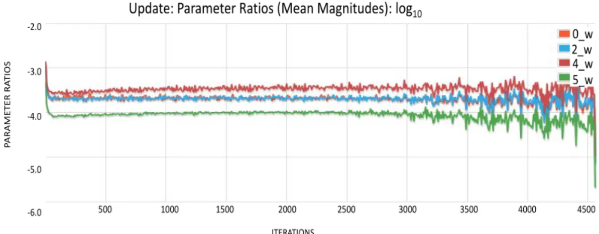
ITERATIONS PA R A ME TE R R AT IOS

Update: Parameter Ratios (Mean Magnitudes): log

0_w

2_w

4_w

5_w

that 1e-2 provided the best learning performance. A decreasing trend in the graph is observed which indicates that the training data is normalized properly. L2 normalization scheme with stochastic gradient descentWt+1=Wt−α δL(θt)is the most appropriate approach for our network training.

Figure 9 depicts ratio of mean magnitudes of the parameters which is suggested to be between -3.0 and -4.0 on a log10 chart. If it is between the suggested range, it indicates that the learning rate and other network hyper-parameters are initialized properly. A divergence of ratio from the suggested range indicates unstable parameter initialization and selection.

Figure 10 shows the layer activation graphs for all weight vectors of each layer. It is observed that the graph tend to stabilize over each iteration and does not suffers from the problem of exploding activations. The stability of the graph after some iterations also shows that proper regularization scheme i.e.λ₂Í

iθi2is adopted. The value ofλis varied from 5 * 1e-2 to 5 * 1e-8 but the value of 5 * 1e-4 provided the best results.

A normal gaussian distribution is observed in the histograms of layer parameters. An approximate gaussian distri-bution in the histogram of weights for different layers shows that the weights have been initialized correctly, updating in each iteration and there is sufficient regularization in the network. An approximate gaussian distribution is also observed in the histogram of layer updates. These updates are the gradients which are generated after applying the regularization, momentum and learning rate. The momentum is given byVt+1=ρvt−α δL(θt)and the value ofρis varied to 0.6, 0.8 and 0.9 for the generated results. The value is finally set to 0.9 for network training. Similar to the layer parameters histogram, an approximate gaussian distribution in the layer updates histogram represents that the network is not prone to exploding gradient problem. This is mainly because of the usage of gradient normalization which we have added in the network.

Performance Characterization:

In order to evaluate the performance of the trained classifier on the proposed parameters, we have used two test datasets comprising of 38 individuals in total. Table 3 shows the confusion matrix depicting the overall performance of the proposed system. The confusion matrix measures the performance of the system by counting the number of true positives, false positive, true negatives and false negatives. We also calculated various evaluations of the proposed

ITERATIONS

0_w

1_w

2_w

3_w

StandardDeviations: log10 (Activations)

4_w

input

F I G U R E 1 0 Layer Activations

system by using four counts such as accuracy, recall, precision and F1 score.

In the first experiment, the test dataset consists of video frames from four different individuals. These video frames contain individuals with varying lighting effects and poses. The four different individuals are represented by four different numeric values in the confusion matrix. It can be seem from the matrix that the classifier performs quite well in distinguishing between different individuals. The individuals with label 0 and label 1 have been classified correctly by 19968 and 19456 times respectively. Similarly, the individuals with label 2 and label 3 are classified correctly by 11264 and 35680 times. The second experiment contains 34 different individuals with varying lighting effects and poses. All the individuals are again represented by 34 different numeric values. The confusion matrix depicted that the classifier performed quite well in this experiment in distinguishing between different individuals. The system generated an overall accuracy of 0.9788 percent.

Some of the video frames are also misclassified by the system as depicted by the false positives. The video frames labeled as label 1 are classified as label 3 for 128 times by the classifier. Also, 320 labels which were labeled as label 3 are classified by the classifier as label 0. Label 3 is also classified 64 times as label 1 by the classifier. Also, for the second experiment some of the labels are miss-classified by the classifier. We believe that these frames are misclassified because of the high variance in the pose of the subject. Various lightning conditions also contributed to the false positives of the system. Since the classifier was trained on the dataset which was captured under controlled lightning conditions, therefore various challenges such as blur and illumination effects are not coped by the system. Tackling these challenges is one of the future works of our system.

The precision of the proposed system, which is the positive prediction value, is recorded to be 0.9709. The proposed system proved to be precise as well as accurate as depicted in the confusion matrix. The recall and F1 score of the system are recorded to be 0.9738 and 0.9783 respectively. Recall can also be referred to as the sensitivity of the system while F1 depicts the overall performance of the system with 0.0 to be the worst score and 1.0 being the best score of the system. Precision and F1 scores for the system are calculated as;

F1 = 2T P/(2T P+F P+F N) ; R ecal l =T P/(T P+F N) (17)

TA B L E 3 Confusion Matrix Classification Scores Accuracy 0.9788 Precision 0.9709 Recall 0.9738 F1 Score 0.9783 {0=[0 x 19968], 1=[1 x 19456, 2 x 512], 2=[0 x 1280, 1 x 256, 2 x 11264 ], 3=[3 x 35680]} {0=0, 1=512, 2=1536, 3=0} {0=1280, 1=256, 2=512, 3=0} {0=19968, 1=19456, 2=11264, 3=35680} {0=67168, 1=68192, 2=75104, 3=52736} {0=[0 x 19, 18], 1=[1 x 20], 2=[16, 2 x 18, 26], 3=[3 x 19, 31], 4=[4 x 20], 5=[5 x 19, 13], 6=[6 x 20], 7=[7 x 20], 8=[8 x 19, 30], 9=[9 x 20], 10=[16, 10 x 19], 11=[11 x 19, 27], 12=[12 x 20], 13=[26, 13 x 19], 14=[14 x 20], 15=[15 x 20], 16=[16 x 20], 17=[17 x 20], 18=[18 x 20], 19=[19 x 20], 20=[20 x 20], 21=[20, 21 x 19], 22=[22 x 20], 23=[23 x 20], 24=[24 x 20], 25=[25 x 20], 26=[26 x 20], 27=[27 x 20], 28=[28 x 20], 29=[24, 29 x 19], 30=[30 x 20], 31=[12 x 2, 31 x 18], 32=[32 x 20], 33=[33 x 19, 7]}

After training the classifier in the cloud, we have downloaded and saved it locally. It is then further used to perform classification of objects from the video streams. The marked or target object which is to be identified from the video streams is passed through the trained classifier after performing all the preprocessing steps on it to make it appropriate for the classifier. The classifier then returns the probabilities of the possible labels for the target object as shown in figure 11 . High probabilities indicate that the target object which was being searched from the video streams is present in that video stream. On the other hand, low probabilities against the video streams indicate the absence of that object in the video streams.

Figure 11 shows the probabilities of some of the objects generated by the classifier. The objects which were provided as input to the trained classifier are listed on the right hand side of the graph. We have shown the results for 10 objects in this graph. Each bar of the graph shows the probability value for each object generated by the classifier. The probabilities approaching to 1 indicates a closer match of the marked object. On the other hand, the probabilities approaching to 0 shows the unavailability of objects in the video stream database.

In order to track a specific object from a number of video streams we check the generated probabilities or matching scores against each video stream. The trained classifier generates a high matching score against the marked object if its training instances is present in the database. We can therefore set an empirically determined threshold on the basis of matching score. The matching scores greater than or equal to the threshold reveal that the object is present in the specific video stream.

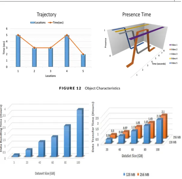
We have also measured the estimated presence time of the object in the video streams and recorded its location as well. The meta-data about the location of the video stream was stored in the database along with the video itself. Once an object is searched in a video stream, its location is also recorded through the meta-data. Figure 12 shows

0 0.2 0.4 0.6 0.8 1 1.2 1 2 3 4 5 6 7 8 9 10 Object1 Object2 Object3 Object4 Object5 Object6 Object7 Object8 Number of experiments Pr obab iliti es

F I G U R E 1 1 Classification of Marked Object

the presence of the object and the trajectory in multiple video streams. The presence of object in the video stream is represented by ‘1’ while its absence is represented by ‘0’. It can be seen that the object remained present throughout in video 1 and video 4. However, in remaining videos it remained there for a fraction of time.

Figure 12 also provides a visual representation about the tracking of the object as it has been mapped on a graphical representation. This graphical representation is actually the summary of multiple videos in which the specific object has been detected. Each bar in the graph represents the amount of time that the marked object has spent at a specific location while its travel movement can be observed by the line graph.

Scalability of the System:

The proposed system is executed on a spark based cloud infrastructure in order to test the scalability and perfor-mance. Spark executes many executors depending upon the configuration and the RDD objects are accessed by each executor in an iteration.

The total size of decoded video frames used in the experiments varied from 5GB to 100GB. The individual video frames are small in size and iterative reduce can perform better on large data files. Due to this, the individual video frames are bundled together by using a batch process and are then moved to cloud for processing. The time required to bundle the data varies with the amount of video frames being considered as shown in Figure 13. This time is directly dependent to the size of the dataset. For a dataset of 10GB to 100GB, the time of a batch process varied from 0.25 hours to 3.8 hours.

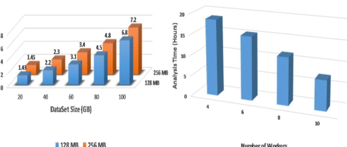
We have measured the time required to transfer the data to cloud data storage. The data transfer time to cloud data storage mainly depends on the bandwidth of the network and the block size of cloud data storage. To have an estimate of the transfer time, we measured the transfer time for various sizes of data and plotted in Figure 14 . It can be observed from the figure that the transfer time varied from 0.36 to 2.18 for a dataset size of 20GB to 100GB. We have also measured this time by changing the cloud storage block size from 128 MB which is the default size to 256MB. However, very little improvement has been recorded in the transfer time by varying the block size.

The training of the proposed system is performed on multiple nodes of the cloud. To have a good estimate of the training time we have executed multiple tests on multiple sizes of datasets and plotted their average execution time in

Sensitivity: Internal 0 1 2 3 4 5 6 1 2 3 4 5 Ti m e (s ec) Locations

Trajectory

Presence Time

F I G U R E 1 3 Data Bundling Time F I G U R E 1 4 Data Transfer Time to Cloud Storage

Figure 15 . The average execution time gives a measure of how much training time on average is required to train the proposed system on a specific size of dataset. The dataset sizes have been varied from 20GB to 100GB to measure the time on various cloud nodes. It has been observed that the execution time increases by increasing the size of dataset.

The total execution time by the system has also been observed on multiple nodes of the cluster by changing the block size. The experiment was repeated by changing the block size to have an estimate that how much effect does block size has on the overall execution time of the system. We have changed the block size from 128 MB (which is the default block size) to 256 MB and repeated the experiment. It can be observed from Figure 15 that the total execution time for 100GB dataset size decreased to 6.8 hours. For 20 GB of dataset size, it took almost 1.43 hours. However, this shows that the block size does not have a major impact on the overall execution time of the system.

F I G U R E 1 5 Analysis Time With Varying Dataset SizesF I G U R E 1 6 Analysis Time With Varying Cloud Nodes

on average on cloud infrastructure, we have executed the system and repeated the experiments by varying the number of cloud nodes. With each experiment we have increased the number of nodes in the cluster and observed the effects on the overall execution time of the system. The overall execution time of the system with an increase in the number of nodes helped to determine the amount of time required to process the total amount of data. It also gives an estimate that how much each node is contributing in the processing the total amount of data. This provides an estimate on how many nodes should be required to process a specific amount of data in a given amount time.

Figure 16 shows that amount of time required by multiple nodes to process the data. It can be seen from the figure that the total amount of time required to process the data decreases with an addition in the number of nodes of the system. Addition of each node in the cloud decreases the overall execution time. However, this also increases the network communication between nodes. More nodes can be added or removed from the system in order to further increase or decrease the overall processing time. However, it should be noted that having few nodes will in-crease the processing cost on each node and having too many nodes will inin-crease the communication cost between them.

We have also observed the effects of data locality on the performance of the overall system. Data locality can play an important role in a deep learning based system performing video analytics. Data locality refers to the avail-ability of image or video data required for processing on multiple nodes of the cluster. If the resilient distributed datasets are not persistant then the replicas of the data block are maintained depending upon the replication factor of distributed file system. This ensures the locality of the data which is helpful for fault tolerance across multiple operations.

We have measured the total time taken by the system for execution with different values of data replication. A good selection of this parameter can help to ensure fault tolerance in the overall execution of the system and can improve the execution time. We have varied the replication factor to different values and observed its effects on the overall percentage of total spawned tasks. Figure 17 shows the values of data replication on the x-axis and the spawned tasks percentage is depicted on the y-axis. It can be observed from the figure that an increase in the value of data replication, increases the locality of data for spawned tasks. However, setting this value to be very high can increase the memory and disk requirements and will also require more network bandwidth.

F I G U R E 1 7 Data Persistance

7

|

CONCLUSION AND FUTURE WORK

A cloud-based video analytics system has been presented and evaluated in this paper. The system is based on con-volutional neural networks whose parameters are optimally tuned for accurate classification of objects from video streams. A comparison of the target object with the pre-trained patterns is made which results in the generation of matching scores. The matching scores greater than an empirically determined threshold reveal the class of the marked object. The system learns features from large amounts of input data by performing training in parallel on a multi-node cluster. The proposed system proved to be robust to classification errors with an accuracy and precision of 97% and 96% respectively. Several factors contributed to achieve high accuracy such as optimal selection of learning rate, regularization, normalization and optimization algorithms. The design of multi-layer network including number of layers and their parameters also played a major role in achieving high accuracy in the system. The proposed system can be used as a general-purpose video analytics system.

In future, we would like to improve the performance of our video analytics system by leveraging other deep learning based models. We will extend the functionality of the system by executing it under complex challenging conditions containing lightning and other variations. We would also like to deploy the proposed system on an in-memory processing cloud coupled with the computation power of GPUs to improve performance and training time.

R E F E R E N C E S

[1] ND4J.https://nd4j.org/;. Accessed: 2018-01-19.

[2] Abdullah T, Anjum A, Tariq MF, Baltaci Y, Antonopoulos N. Traffic monitoring using video analytics in clouds. In: Proceed-ings of the 2014 IEEE/ACM 7th International Conference on Utility and Cloud Computing IEEE Computer Society; 2014. p. 39–48.

[3] Ahmed E, Jones M, Marks TK. An improved deep learning architecture for person re-identification. In: Proceedings of the IEEE Conference on Computer Vision and Pattern Recognition; 2015. p. 3908–3916.

[5] Carrasco M, Pizarro L, Mery D. Bimodal Biometric Person Identification System Under Perturbations. In: Mery D, Rueda L, editors. Advances in Image and Video Technology Berlin, Heidelberg: Springer Berlin Heidelberg; 2007. p. 114–127. [6] Dhanalakshmi A, Srinivasan B. Improved Person Identification System using Face Biometric Detection. International

Journal of Advanced Networking and Applications 2013;4(5):1731.

[7] Fox N, Gross R, de Chazal P, Cohn J, Reilly R. Person identification using multi-modal features: Speech, lip, and face. In: ACM Multimedia Workshop in Biometrics Methods and Applications (WBMA 2003); 2003. p. 25 – 32.

[8] Geiger JT, Kneißl M, Schuller BW, Rigoll G. Acoustic gait-based person identification using hidden Markov models. In: Proceedings of the 2014 Workshop on Mapping Personality Traits Challenge and Workshop ACM; 2014. p. 25–30. [9] Ikram A, Anjum A, Hill R, Antonopoulos N, Liu L, Sotiriadis S. Approaching the Internet of things (IoT): a modelling,

analy-sis and abstraction framework. Concurrency and Computation: Practice and Experience 2015;27(8):1966–1984. [10] Ioffe S, Szegedy C. Batch normalization: Accelerating deep network training by reducing internal covariate shift. arXiv

preprint arXiv:150203167 2015;.

[11] Karpathy A, Toderici G, Shetty S, Leung T, Sukthankar R, Fei-Fei L. Large-scale video classification with convolutional neural networks. In: Proceedings of the IEEE conference on Computer Vision and Pattern Recognition; 2014. p. 1725– 1732.

[12] Lee SU, Cho YS, Kee SC, Kim SR. Real-Time Facial Feature Detection for Person Identification System. In: MVA; 2000. p. 148–151.

[13] Levi G, Hassner T. Age and gender classification using convolutional neural networks. In: Proceedings of the IEEE Con-ference on Computer Vision and Pattern Recognition Workshops; 2015. p. 34–42.

[14] Li W, Zhao R, Xiao T, Wang X. Deepreid: Deep filter pairing neural network for person re-identification. In: Proceedings of the IEEE Conference on Computer Vision and Pattern Recognition; 2014. p. 152–159.

[15] van Lingen F, Steenberg C, Thomas M, Anjum A, Azim T, Khan F, et al. The Clarens Web service framework for distributed scientific analysis in grid projects. In: Parallel Processing, 2005. ICPP 2005 Workshops. International Conference Work-shops on IEEE; 2005. p. 45–52.

[16] Lu Y, Fleury A, Boonaert J, Lecoeuche S, Ambellouis S. Online person identification and new person discovery using appearance features. In: 2015 IEEE International Conference on Evolving and Adaptive Intelligent Systems (EAIS); 2015. p. 1–8.

[17] McClatchey R, Branson A, Anjum A, Bloodsworth P, Habib I, Munir K, et al. Providing traceability for neuroimaging anal-yses. International journal of medical informatics 2013;82(9):882–894.

[18] Miller H, Haller P, Burmako E, Odersky M. Instant pickles: generating object-oriented pickler combinators for fast and extensible serialization. In: ACM Sigplan Notices, vol. 48 ACM; 2013. p. 183–202.

[19] N CR, Rajiv R, Anton B, F DRCA, Rajkumar B. CloudSim: a toolkit for modeling and simulation of cloud computing environments and evaluation of resource provisioning algorithms. Software: Practice and Experience;41(1):23–50.

https://onlinelibrary.wiley.com/doi/abs/10.1002/spe.995.

[20] Nanni L, Munaro M, Ghidoni S, Menegatti E, Brahnam S. Ensemble of different approaches for a reliable person re-identification system. Applied Computing and Informatics 2016;12(2):142 – 153. http://www.sciencedirect.com/

science/article/pii/S2210832715000046.

[21] Nikolay G, Rajkumar B. Inter-Cloud architectures and application brokering: taxonomy and survey. Software: Practice and Experience;44(3):369–390.https://onlinelibrary.wiley.com/doi/abs/10.1002/spe.2168.

[23] Simonyan K, Zisserman A. Very deep convolutional networks for large-scale image recognition. arXiv preprint arXiv:14091556 2014;.

[24] Spark A, Apache Spark: Lightning-fast cluster computing. Retrieved from Apache Spark: http://spark.apache.org; 2016. [25] Steenberg C, Bunn J, Legrand I, Newman H, Thomas M, van Lingen F, et al. The Clarens Grid-enabled Web Services

Framework: Services and Implementation. In: Proceedings of the CHEP, vol. 4; 2004. .

[26] Van Lingen F, Thomas M, Azim T, Chitnis I, Anjum A, Bourilkov D, et al. Grid enabled analysis: architecture, prototype and status 2005;.

[27] Waheed Z, Akram MU, Waheed A, Khan MA, Shaukat A, Ishaq M. Person identification using vascular and non-vascular retinal features. Computers & Electrical Engineering 2016;53:359–371.

[28] Yale. The Extended Yale Face Database B (Cropped) 2001;http://vision.ucsd.edu/~iskwak/ExtYaleDatabase/

ExtYaleB.html, accessed: 2018-01-19.

[29] Yaseen MU, Anjum A, Antonopoulos N. Spatial Frequency Based Video Stream Analysis for Object Classification and Recognition in Clouds. In: 2016 IEEE/ACM 3rd International Conference on Big Data Computing Applications and Tech-nologies (BDCAT); 2016. p. 18–26.

[30] Yaseen MU, Anjum A, Rana O, Antonopoulos N. Deep Learning Hyper-Parameter Optimization for Video Analytics in Clouds. IEEE Transactions on Systems, Man, and Cybernetics: Systems 2018;p. 1–12.

[31] Yaseen MU, Anjum A, Antonopoulos N. Modeling and Analysis of a Deep Learning Pipeline for Cloud based Video An-alytics. In: Proceedings of the Fourth IEEE/ACM International Conference on Big Data Computing, Applications and Technologies ACM; 2017. p. 121–130.

[32] Yaseen MU, Anjum A, Rana O, Hill R. Cloud-based scalable object detection and classification in video streams. Future Generation Computer Systems 2018;80:286–298.

[33] Yi D, Lei Z, Liao S, Li SZ. Deep metric learning for person re-identification. In: Pattern Recognition (ICPR), 2014 22nd International Conference on IEEE; 2014. p. 34–39.

[34] Zamani AR, Zou M, Diaz-Montes J, Petri I, Rana O, Anjum A, et al. Deadline constrained video analysis via in-transit computational environments. IEEE Transactions on Services Computing 2017;.