ON A MOLLIFIER OF THE PERTURBED RIEMANN ZETA-FUNCTION PATRICK K ¨UHN, NICOLAS ROBLES, AND DIRK ZEINDLER
Abstract. The mollification ζ(s) +ζ0(s) put forward by Feng is computed by analytic methods
coming from the techniques of the ratios conjectures ofL-functions. The current situation regarding the percentage of non-trivial zeros of the Riemann zeta-function on the critical line is then clarified.
1. Introduction
1.1. Statement of the results. The Riemann zeta-functionζ(s) is defined by the Dirichlet series ζ(s) =P∞
n=1n−s fors=σ+it,σ >1 andt∈R. The functional equation of ζ(s) is given by
ξ(s) =ξ(1−s), where
ξ(s) =H(s)ζ(s) and H(s) = 1
2s(s−1)π
−s/2Γ
s 2
.
This allows us to perform a meromorphic continuation to the whole complex plane except ats= 1 where ζ(s) has a simple pole with residue equal to 1. The connection with number theory comes from the Euler product
ζ(s) =Y
p
(1−p−s)−1,
for Re(s)>1, and where the product is taken over all the primesp. It is well-known from Riemann and from von Mangoldt that the non-trivial zeros ρ=β+iγ of ζ(s) are located inside the critical strip 0< β <1. Moreover, ifN(T) denotes the number of such zeros up to height 0≤γ < T then
N(T) = T 2π
log T 2π −1
+7
8 +S(T) +O
1 T
,
where
S(T) = 1 π argζ
1 2+it
logT,
as T → ∞, see e.g. [13, 16] for properties of ζ(s). To state the results, we let N0(T) denote the
number of non-trivial zeros up to height T >0 such that β= 1/2. Similarly, letN0∗(T) denote the number such zeros which are also simple. We then define
κ= lim inf
T→∞
N0(T)
N(T) and κ
∗
= lim inf
T→∞
N0∗(T) N(T).
The history behind the value of κ can be found in [3, 8, 14]. The main breakthroughs were as follows. In 1942, Selberg [15] established that 0 < κ ≤ 1. Levinson later showed in 1974 that κ ≥ .3474. This was improved by Conrey to κ ≥ .4088 in 1989 and later refined by Bui, Conrey and Young [3] to κ ≥ .4105, and shortly afterward by Feng [8] to κ ≥ .4127. It should be noted that both results are improvements of κ≥.4088 and are independent of each other.
2010Mathematics Subject Classification. Primary: 11M36; Secondary: 11M06, 11N64.
Keywords and phrases. Riemann zeta-function, mollifier, zeros on the critical line, ratios conjecture technique, generalized von Mangoldt function.
The second author, Roy and Zaharescu [14] as well as Bui [2] brought up a point regarding the strength of Feng’s result. In [14], it was explained that κ ≥ .4107, unconditionally, using Feng’s mollifier. However, the computation of the mixed terms of the mollifiers of Conrey and of Feng was not carried through explicitly.
It should also be remarked that Bui [2] suggests that the bound obtained in this paper can be attained using the twisted second moment of the Riemann zeta-function due to Balasubramanien
et. al. [1] and that he also suggests an alternative argument that could lead to the boundκ > .41098.
In this paper, we close this gap and we explain Feng’s brilliant choice in the context of the pow-erful technology developed in [3, 17]. These ideas come from the ratios conjectures ofL-functions due to Conrey, Farmer and Zirnbaeuer [6] as well as to Conrey and Snaith [7]. It should be noted that Feng’s methodology to obtain the main terms of his theorem consisted on an ingenious combi-nation of elementary methods, namely induction and Mertens’ formula, applied to Conrey’s result [5]. On the other hand, this choice of methods blurred a bit the length the mollifier was allowed to take. Other than choosing the same mollifier, our computations do not overlap and the methods are quite different.
Lastly, the closing of this gap will clarify the situation of the percentage of non-trivial zeros on the critical line when one attaches Feng’s second-piece mollifier to Conrey’s.
1.2. Choice of mollifiers. LetQ(x) be a real polynomial satisfyingQ(0) = 1, Q(x) +Q(1−x) = constant, and define
V(s) =Q
− 1 L
d ds
ζ(s), (1.1)
where for largeT,
L= logT.
If ψ(s) is a mollifier, then it is well-known from the work of Levinson [12] and of Conrey [5] that Littlewood’s lemma [16,§9.9] followed by the arithmetic and geometric mean inequalities yields
κ≥1− 1 Rlog
1 T
Z T
1
|V ψ(σ0+it)|2dt
+o(1), (1.2)
where σ0 = 1/2−R/L, and R is a bounded positive real number to be chosen later. Following
Feng [8], we will choose a mollifier of the form
ψ(s) =ψ1(s) +ψ2(s),
where ψ1 is the mollifier considered by Conrey. Let P1(x) = Pjajxj be a certain polynomial
satisfying P1(0) = 0,P1(1) = 1, and lety1 =Tθ1 where 0< θ1<4/7. We adopt the notation
P1[n] =P1
log(y1/n)
logy1
for 1≤n≤y1. By convention, we setP1[x] = 0 forx≥y1. Then ψ1(s) is given by
ψ1(s) = X
h≤y1
µ(h)hσ0−1/2 hs P1[h],
(1.3)
whereµ(n) is the M¨obius function. For the second mollifier, we take
ψ2(s) = X
k6y2
µ(k)kσ0−1/2 ks
K X
`=2 X
p1···p`|k
logp1· · ·logp`
log`y2
P`[k].
Here K ≥2 is an integer of our choice and p1,· · ·, p` are distinct primes. Also we need P`(0) = 0
for`= 2,· · · , K. In this case y2 =Tθ2 where 0< θ2 <1/2.
Remark 1.1. It will become clear in the calculation of the crossterm integral between ψ1 and ψ2
that one needs θ1+θ2 <1−ε. Therefore, if θ1 increases, thenθ2 decreases unless some difficult
work is done to pushθ2 back to its original (or higher) value. See the comments between Theorem
1.1 and Theorem 1.2 for more details.
The reason behind this choice is that Feng wishes to mollify not only ζ(s) but also logζ0(s)T, which is the second term coming from (1.1). This is accomplished by looking at
1
ζ(s) + ζlog0(s)T = 1 ζ(s) −
1 logT
ζ0 ζ2(s) +
1 log2T
(ζ0)2 ζ3 (s)−
1 log3T
(ζ0)3
ζ4 (s) +· · ·.
(1.5)
When kis a square-free positive integer, then one has
(µ∗Λ∗`)(k) = (−1)`µ(k) X
p1···p`|k
logp1· · ·logp`,
where f ∗g denotes the Dirichlet convolution of arithmetic functions f and g. Here Λ∗` stands for convolving the von Mangoldt function Λ(n) with itself exactly ` times. Ifk contains a square divisor, then, as remarked by Feng [8], the coefficients aj resulting from (1.5) contribute a lower
order to the mean value integralsI11,I12andI22related toκin (1.2) (see below for exact definitions
of these I-integrals).
1.3. Numerical evaluations. We will prove the following.
Theorem 1.1. We obtain with θ1 =θ2 = 1/2−ε
κ≥.369927 and κ∗≥.359991, unconditionally.
Using the work of Iwaniec and Deshouillers [10, 11], Conrey [5] was able to push the size of the mollifier ψ1 toθ1 <4/7−ε. In the light of Lemma 2.1 and (3.9) below, we requireθ1+θ2 <1 in
our argumentation. The points brought up in [2] and [14] show that some difficult work is needed if one takes θ1+θ2 >1. Theorem 1.1 utilizes θ1, θ2 <1/2−ε. However, if we take θ1 <4/7−ε
and θ2 <3/7−ε, then we get
Theorem 1.2. We obtain with θ1 <4/7−εand θ2<3/7−ε
κ≥.410725 and κ∗≥.403211, unconditionally.
It should therefore be stressed that Theorem 1.1 is an improvement of the last theorem to ever useθ1 = 1/2−ε, namely the first corollary of [4], where it was shown that κ≥.3658.
The method sketched in [3, 14] to deal with multiple piece mollifiers carries through and our main result is as follows.
Theorem 1.3. Suppose thatθ1+θ2 = 1−εwith θ1<4/7 and θ2 <1/2 and ε >0 small. Then
1 T
Z T
1
|V ψ(σ0+it)|2dt=c(P1, P`, Q, R, θ1, θ2) +o(1),
We use Mathematicato numerically evaluatec(P1, P`, Q, R,1/2,1/2) with the following choices
of parameters. WithK = 3,R= 1.3,
Q(x) =.481936 +.632349(1−2x)−.144698(1−2x)3+.0304136(1−2x)5,
P1(x) =x+.225339x(1−x)−1.01137x(1−x)2+.174004x(1−x)3−.100235x(1−x)4,
P2(x) = 1.05138x+.284201x2,
P3(x) =.222032x−.13254x2,
we have κ≥.369927. To getκ∗ ≥.359991, we takeK = 3,R = 1.2, Q(x) =.476202 +.523798(1−2x),
P1(x) =x+.0531913x(1−x)−.594999x(1−x)2−.00107597x(1−x)3−.0761954x(1−x)4,
P2(x) =.896567x−.0297464x2,
P3(x) =.0699271x−.108964x2.
We also useMathematicato numerically evaluatec(P1, P`, Q, R,4/7,3/7) with the following choices
of parameters. WithK = 3,R= 1.295,
Q(x) =.492203 +.621972(1−2x)−.148163(1−2x)3+.033988(1−2x)5,
P1(x) =x+.229117x(1−x)−2.932318x(1−x)2+ 4.856163x(1−x)3−2.390999x(1−x)4
P2(x) =−.072644x+ 1.559440x2
P3(x) =.701568x−.554403x2
we have κ≥.410725. To getκ∗ ≥.403211, we takeK = 3,R = 1.109, Q(x) =.485034 +.514966(1−2x),
P1(x) =x+.0486916x(1−x)−2.02526x(1−x)2+ 3.43611x(1−x)3−1.62355x(1−x)4,
P2(x) =−.034431x+ 1.09223x2,
P3(x) =.479296x−0.385868x2.
An interesting question to ask is: what would have happened if Feng had published his mollifier before Conrey’s increment of θ1 from 1/2 to 4/7. Since this has not been remarked before in the
literature, we take the chance to answer it. Ifψ1 andψ2 are kept at 1/2−ε, then Feng’s piece adds
an additional 0.4127% to Conrey’s 36.58% as shown in the table below.
θ1 θ2 %
1/2 1/2 36.58% + 0.4127% 4/7 3/7 40.88% + 0.1925%
Table 1. % according to sizes of θ
Sinceψ2 is the perturbation ofψ1, it behooves us to takeθ1as large as possible (4/7) at the cost
of sacrificingθ2 to 3/7 which only adds 0.1925%.
1.4. The smoothing argument. The idea of smoothing the mean value integrals was introduced in [3, 17] and it helps substantially in our calculations. Let w(t) be a smooth function satisfying the following properties:
(a) 0≤w(t)≤1 for all t∈R,
(b) w has compact support in [T /4,2T],
This allows us to re-write Theorem 1.3 as follows.
Theorem 1.4. Suppose that θ1 = 1/2−ε and θ2 = 1/2−ε for ε >0 small. For any w satisfying
conditions (a), (b) and (c) and σ0 = 1/2−R/L, Z ∞
−∞
w(t)|V ψ(σ0+it)|2dt=c(P1, P`, Q, R, θ1, θ2)wb(0) +O(T /L),
uniformly for R1, where c(P1, P`, Q, R, θ1, θ2) =c11+ 2c12+c22 and the cij are given by (1.6),
(1.7)and (1.8).
How to deal with a two-piece mollifier was explained in [3, 8]. In [14] a 4-piece mollifier was studied. The idea is to open the square in the integrand to get
Z
|V ψ|2=
Z
|V ψ1|2+ Z
|V|2ψ1ψ2+ Z
|V|2ψ1ψ2+ Z
|V ψ2|2
=I11+I12+I12+I22.
We will compute these integrals in the next sections. The integralI12 is asymptotically real, thus
I21 follows from I12, i.e. I12∼I21.
1.5. The main terms. The main terms coming from integrals I11,I12 and I22 are now stated as
theorems.
Theorem 1.5 (Conrey). Suppose θ1 <4/7. Then Z ∞
−∞
w(t)|V ψ1(σ0+it)|2dt∼c11(P1, Q, R, θ1)wb(0) +O(T /L)
uniformly for R1, where
c11(P1, Q, R, θ1) = 1 +
1 θ1
Z 1
0 Z 1
0
e2Rv
d dxe
RθxP
1(x+u)Q(v+θx)|x=0 2
dudv. (1.6)
Let (`)k=`(`−1)·. . .·(`−k+ 1) denote the Pochhammer symbol. Theorem 1.6. Suppose θ1+θ2 = 1−εwhere θ1 <4/7 and θ2<1/2. Then
Z ∞
−∞
w(t)V ψ1ψ2(σ0+it)dt∼c12(P1, P`, Q, R, θ1, θ2)wb(0) +O(T /L)
uniformly for R1, where
c12(P1, P`, Q, R, θ1, θ2) = K X
`=2
(−1)` (`−1)!
Z 1
0
(1−u)`−1P1(u)P`(u)du
−θ1−θ2 θ1
K X
`=2
(−1)` `!
Z 1
0
(1−u)`−1P01
1−(1−u)θ2 θ1
P`(u)du
+ 1 θ1
K X
`=2
(−1)` `!
d2 dxdy
eR(θ1x+θ2y)
Z 1
0 Z 1
0
e2Rv(1−u)`
×P1
x+ 1−(1−u)θ2 θ1
P`(y+u)Q(θ2y+v)Q(θ1x+v)dudv
x=y=0
. (1.7)
Theorem 1.7. Suppose θ2<1/2. Then Z ∞
−∞
uniformly for R1, where
c22(P`, Q, R, θ2) = K X
`1=2
K X
`2=2
min(`1,`2)
X
k=0
(−1)`1+`2−2k
`1
k
(`2)k
× 2
`1+`2−2k
(`1+`2−1)! Z 1
0
(1−u)`1+`2−1P
`1(u)P`2(u)du
+ 1 θ2
K X
`1=2
K X
`2=2
min(`1,`2)
X
k=0
(−1)`1+`2−2k
`1
k
(`2)k
2`1+`2−2k (`1+`2)!
d2 dxdy
eRθ2(x+y)
×
Z 1
0 Z 1
0
e2Rv(1−u)`1+`2P
`1(x+u)P`2(y+u)Q(v+θ2x)Q(v+θ2y)dudv
x=y=0
. (1.8)
Remark 1.2. Note that in [8],c11,c12 andc22 are all mixed into one single theorem and it is not
immediately clear how to separate each individual c-term.
The smoothing argument is helpful because we can easily deduce Theorem 1.3 from Theorem 1.4 and so on. By having chosen w(t) to satisfy conditions (a), (b) and (c) and in addition to being an upper bound for the characteristic function of the interval [T /2, T], and with support [T /2−∆, T + ∆], we get
Z T
T /2
|V ψ(σ0+it)|2dt≤c(P1, P`, Q, R, θ1, θ2)wb(0) +O(T /L).
Note that wb(0) =T /2 +O(T /L). We similarly get a lower bound. Summing over dyadic segments
gives the full result.
1.6. The shift parameters α and β. Rather than working directly with V(s), we shall instead consider the following three general shifted integrals
I11(α, β) = Z ∞
−∞
w(t)ζ(12+α+it)ζ(21+β−it)ψ1ψ1(σ0+it)dt,
I12(α, β) = Z ∞
−∞
w(t)ζ(12+α+it)ζ(21+β−it)ψ1ψ2(σ0+it)dt,
I22(α, β) = Z ∞
−∞
w(t)ζ(12+α+it)ζ(21+β−it)ψ2ψ2(σ0+it)dt.
The computation is now reduced to proving the following three lemmas.
Lemma 1.1. We have
I11=c11(α, β)wb(0) +O(T /L),
uniformly for α, βL−1, where
c11(α, β) = 1 +
1 θ1
d2 dxdy
y1−βx−αy
Z 1
0 Z 1
0
T−v(α+β)P1(x+u)P1(y+u)dudv
x=y=0
. (1.9)
Lemma 1.2. We have
I12=c12(α, β)wb(0) +O(T /L),
uniformly for α, βL−1, where
c12(α, β) = K X
`=2
(−1)` (`−1)!
Z 1
0
−θ1−θ2 θ1
K X
`=2
(−1)` `!
Z 1
0
(1−u)`P10
1−(1−u)θ2 θ1
P`(u)du
+ 1 θ1
K X
`=2
(−1)` `!
d2 dxdy
y1−βxy2−αy
×
Z 1
0 Z 1
0
T−v(α+β)(1−u)`P1
x+ 1−(1−u)θ2 θ1
P`(y+u)dudv
x=y=0
. (1.10)
Lemma 1.3. We have
I22=c22(α, β)wb(0) +O(T /L),
uniformly for α, βL−1, where
c22(α, β) = K X
`1=2
K X
`2=2
min(`1,`2)
X
k=0
(−1)`1+`2−2k
`1
k
(`2)k
× 2
`1+`2−2k
(`1+`2−1)! Z 1
0
(1−u)`1+`2−1P
`1(u)P`2(u)du
+ 1 θ2
K X
`1=2
K X
`2=2
min(`1,`2)
X
k=0
`1
k
(`2)k(−1)
`1+`2−2k2
`1+`2−2k
(`1+`2)!
× d
2
dxdy
y2−βx−αy
Z 1
0 Z 1
0
T−v(α+β)(1−u)`1+`2P
`1(x+u)P`2(y+u)dudv
x=y=0
. (1.11)
To get Theorems 1.5, 1.6 and 1.7 we use the following technique. Let I? denote either of the
integrals in questions, and note that
I? =Q
− 1 logT
d dα
Q
− 1 logT
d dβ
I?(α, β)
α=β=−R/L
.
Since I?(α, β) and c?(α, β) are holomorphic with respect to α, β small, the derivatives appearing
in the equation above can be obtained as integrals of radii L−1 around the points −R/L, using Cauchy’s integral formula. Since the error terms hold uniformly on these contours, the same error terms that hold for I?(α, β) also hold for I?. That the above differential operator onc?(α, β) does
indeed givec? follows from
Q
−
1 logT
d dαX
−α
=Q
logX logT
X−α.
Note that from the above equation we get
Q
−
1 logT
d dα
Q
−
1 logT
d dβ
y1−βxy−2αyT−v(α+β)=Q
logyy2Tv logT
Q
logyx1Tv logT
y1−βxy2−αyT−v(α+β)
=Q(θ2y+v)Q(θ1x+v)y1−βxy
−αy 2 T
−v(α+β),
as well as
Q
−
1 logT
d dα
Q
−
1 logT
d dβ
y2−βx−αyT−v(α+β)=Q
logy2yTv logT
(y2yTv)−αQ
logy2xTv logT
(yx2Tv)−β
=Q(θ2y+v)Q(θ2x+v)y
−βx−αy 2 T
Hence using the differential operatorsQ((−1/logT)d/dα) andQ((−1/logT)d/dβ) on the last line of c12(α, β) we get
d2 dxdy
y−1βxy2−αy
Z 1
0 Z 1
0
T−v(α+β)(1−u)`P1
x+ 1−(1−u)θ2 θ1
P`(y+u)Q(θ2y+v)Q(θ1x+v)dudv
x=y=0
.
Theorem 1.6 then follows by setting α = β = −R/L and using Tz/L = Tz/logT =ez. Similarly,
when we use the differential operatorsQ((−1/logT)d/dα) andQ((−1/logT)d/dβ) on the last line of c22(α, β) it becomes
d2 dxdy
eRθ2(x+y)
Z 1
0 Z 1
0
e2Rv(1−u)`1+`2P
`1(x+u)P`2(y+u)Q(v+θ2x)Q(v+θ2y)dudv
x=y=0
.
The same substitutions yield Theorem 1.7.
2. Preliminary results
2.1. Results from complex analysis. The following results are needed throughout the paper.
Lemma 2.1. Suppose that w(t) satisfies conditions (a), (b) and (c) and that h, k are positive integers withhk≤T2θ withθ <1/2, andα, β L−1. Moreover, set
gα,β(s, t) =π−s
Γ(12(12 +α+s+it))Γ(12(12+β+s−it)) Γ(12(12 +α+it))Γ(12(12+β−it)) , as well as
Xα,β,t=πα+β
Γ(12(12 −α−it))Γ(12(12−β+it)) Γ(12(12 +α+it))Γ(12(12+β−it)). Then one has
Z ∞
−∞
w(t)
h k
−it
ζ(12 +α+it)ζ(12 +β−it)dt= X
hm=kn
1 m1/2+αn1/2+β
Z ∞
−∞
Vα,β(mn, t)w(t)dt
+ X
hm=kn
1 m1/2−βn1/2−α
Z ∞
−∞
V−β,−α(mn, t)Xα,β,tw(t)dt+OA(T−A),
where
Vα,β(x, t) =
1 2πi
Z
(1)
G(s)
s gα,β(s, t)x
−sds, G(s) =es2
p(s) and p(s) = (α+β)
2−(2s)2
(α+β)2 .
Proof. See Lemma 5 of [17]. They key point is that non-diagonal terms hm 6= kn can safely be
absorbed in the error terms.
Lemma 2.2. Suppose 0< δL−1,β L−1 and β < δ. For some ν(log logy)−1 we have Υ := 1
2πi
Z
(δ)
1 ζ(1 +β+u)
ζ0
ζ(1 +β+u)
`−r
y?
n
u du
uj+1
= (−1)`−r 1 2πi
I
(β+u)1−`+ry? n
u du
uj+1 +O(L
`−r−2+j) +O
y?
n
−ν
Lε
,
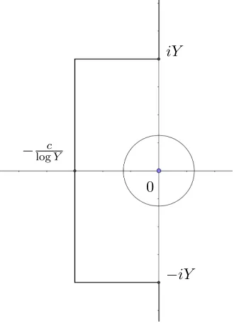
Proof. This follows a similar procedure to Lemma 6.1 of [3] where the zero-free region ofζ is used. LetY =o(T) be a large parameter to be chosen later. By Cauchy’s theorem, Υ is equal to the sum of residues atu= 0 andu=−β plus integrals over the line segmentsγ1={s=it:t∈R,|t| ≥Y},
γ2 ={s=σ±iY :−c/logY ≤σ ≤0}, and γ3 ={s=−c/logY +it:|t| ≤Y}, where c is some
fixed positive positive constant such thatζ(1 +β+u) has no zeros in the region on the right-hand side of the contour determined by theγi’s. Another requirement oncis that the estimate (see [16,
0 iY
[image:9.612.224.389.164.392.2]−iY −logcY
Figure 2.1. Curveγ in the proof of Lemma 2.2.
Theorem 3.11]) 1/ζ(σ+it) log(2 +|t|) holds in this region and ζ0/ζ(σ+it) log(4 +|t|) (see [13, Theorem 6.7]). Then, one has
Z
γ1
Z ∞
Y
log(t)1+`−r
tj+1 dt
log(Y)1+`−r
Yj ,
sincej≥3. Moreover, sincen≤y? Z
γ2
Z 0
−c/logY
log(Y)1+`−ry? n
x 1
Yj+1 dx
log(Y)`−r Yj+1 ,
and finally
Z
γ3
Z Y
−Y
log(4 +|t|)`−r+1(y?/n)
−c/logY
c2/log2Y +t2 dtlog(Y)
`−r+j(y
?/n)−c/logY.
Appropriately choosing Y (logy?) gives an error of size O((log logy?)`−r+j) = O(logy?). The
next step is to sum the residues. This sum can now be expressed as 1
2πi
I 1
ζ(1 +β+u)
ζ0
ζ(1 +β+u)
`−ry ?
n
u du
uj+1,
where the contour is now a small circle Ω of radius 1/L around the origin such that −β ∈ Ω. Since the radius of the circle is tending to zero, we can use the Laurent expansions
1
ζ(s) =s−1 +O((s−1)
2) and ζ0
ζ(s) =− 1
to finally obtain 1 2πi
I
1 ζ(1 +β+u)
ζ0
ζ (1 +β+u)
`−r
y?
n
u du
uj+1
= 1
2πi
I
(β+u+O(u2))
−
1
β+u +O(1)
`−r y?
n
u du
uj+1.
Using the binomial theorem and a direct estimate gives, we get that the above is equal to
(−1)`−r
I
(β+u)1−`+ry? n
u du
uj+1 +O(L
j+`−r−2),
which is the desired main term of the lemma.
This integral can be computed exactly. To do this, note that for any integerk≥1, one has
qu(β+u)k= d
k
dyke
βy(eyq)u
y=0
.
Hence, one arrives at and where we temporarily setq=y?/n
Υ = (−1)`−r 1 2πi
I
d1−`+r dy1−`+re
βy(eyq)u
y=0
du
uj+1 = (−1)
`−r d1−`+r
dy1−`+re βy 1
2πi
I
(eyq)u|y=0
du uj+1
= (−1)
`−r
j!
d1−`+r dy1−`+re
βyy+ logy?
n
j
y=0
, (2.1)
by Cauchy’s integral theorem.
2.2. Combinatorial results. When computing the crossterm of ψ1 and ψ2 the following result
will be needed. This generalizes [8, Lemma 8] which is the particular caseh1=h2 =h. Lemma 2.3. For h1 and h2 square-free, we have
Q(`1, `2) :=
X
p1p2···p`1|h1
logp1logp2· · ·logp`1
X
q1q2···q`2|h2
logq1logq2· · ·logq`2
=
min{`1,`2}
X
k=0
k!
`1
k
`2
k
X
p1p2···pkq1q2···q`1−kr1r2···r`2−k|h1h2/gcd(h1,h2)
p1p2···pk|gcd(h1,h2)
q1···q`1−k|h1
r1···r`2−k|h2
×
k Y
f=1
log2pf
`1−k
Y
f=1
logqf
`2−k
Y
f=1
logrf
,
Here the p’s, theq’s and the r’s are all distinct primes.
Proof. We may write Q(`1, `2) =
X
p1p2···p`1|h1
pa6=pb
logp1logp2· · ·logp`1
X
q1q2···q`2|h2
qa6=qb
logq1logq2· · ·logq`2
=`1!`2!
X
p1p2···p`1|h1
p1<p2<···<p`1
logp1logp2· · ·logp`1
X
q1q2···q`2|h2
q1<q2<···<q`2
=`1!`2!
min{`1,`2}
X
k=0
X
p1p2···pkq1q2···q`1−kr1r2···r`2−k|h1h2/gcd(h1,h2)
p1p2···pk|gcd(h1,h2), q1···q`1−k|h1, r1···r`2−k|h2
p1<p2<···<pk, q1<q2<···<q`1−k, r1<r2<···<r`2−k
× log2p1· · ·log2pk
logq1· · ·logq`1−k
logr1· · ·logr`2−k
=
min{`1,`2}
X
k=0
`1!`2!
k!(`1−k)!(`2−k)!
X
p1p2···pkq1q2···q`1−kr1r2···r`2−k|h1h2/gcd(h1,h2)
p1p2···pk|gcd(h1,h2), q1···q`1−k|h1, r1···r`2−k|h2
× log2p1· · ·log2pk
logq1· · ·logq`1−k
logr1· · ·logr`2−k
.
Using the definition of the binomial coefficient completes the proof.
2.3. Generalized von Mangoldt functions and Euler-MacLaurin summations. Recall that for a positive integerk, the generalized von Mangoldt function Λk(n) is defined [9] by the Dirichlet
convolution
Λk(n) = (µ∗logk)(n),
so that Λ1(n) = Λ(n). The generating series is
∞
X
n=1
Λk(n)
ns = (−1) kζ(k)
ζ (s),
for Re(s)>1 and hereζ(k) stands for thek-th derivative ofζ with respect tos. By looking at d
ds
ζ(k) ζ (s)
= ζ
(k+1)
ζ (s)− ζ0
ζ(s) ζ(k)
ζ (s) for Re(s)>1, we see that
Λk+1(n) = Λk(n) log(n) + (Λ∗Λk)(n),
and in particular fork= 1
Λ2(n) = Λ(n) log(n) + (Λ∗Λ)(n).
(2.2)
Lemma 2.4. We have for smooth functions F and G in the interval [0,1], 3 ≤ z ≤ x, and |s| ≤(logx)−1
X
n≤z
Λ(n) logn n1+s F
log(x/n) logx
H
log(z/n) logz
=log
2z
zs Z 1
0
(1−u)F
1−(1−u)logz logx
H(u)zusdu
+O(logz). Proof. Start by setting
Ψ(z, x) :=X
n≤z
Λ(n) logn n1+s F
log(x/n) logx
H
log(z/n) logz
and ψ(x) :=X
n≤x
Λ(n).
By applying the Abel summation formula, one gets
Ψ(z, x) =ψ(z)logz z1+sF
log(x/z) logx
H(0)−
Z z
1
ψ(u) d du
logu u1+sF
log(x/u) logx
H
log(z/u) logz
du
=−
Z z
1
ψ(u) d du
logu u1+sF
log(x/u) logx
H
log(z/u) logz
du+O(logz)
=−
Z z
1
ψ(u)1−(1 +s) logu
u2+s F
log(x/u) logx
H
log(z/u) logz
−
Z z
1
ψ(u)logu u1+s
d duF
log(x/u) logx
H
log(z/u) logz
du
−
Z z
1
ψ(u)logu u1+sF
log(x/u) logx
d duH
log(z/u) logz
du+O(logz)
= log
2z(1 +s)
zs
Z 1
0
ψ(z1−b)(1−b)F
1−(1−b)logz logx
H(b)zbs+b−1db
+O
logz
Z z
1
ψ(u) 1 u2+|s|du
+ 1
logx
Z z
1
ψ(u)logu u2+sF
0
log(x/u) logx
H
log(z/u) logz
du
+ 1
logz
Z z
1
ψ(u)logu u2+sF
log(x/u) logx
H0
log(z/u) logz
du+O(logz)
= log
2z(1 +s)
zs
Z 1
0
ψ(z1−b)(1−b)F
1−(1−b)logz logx
H(b)zbs+b−1db+O(logz)
= log
2z
zs Z 1
0
ψ(z1−b)(1−b)F
1−(1−b)logz logx
H(b)zbs+b−1db
+O
logz
Z 1
0
ψ(z1−b)(1−b)zbs+b−1db
+O(logz)
= log
2z
zs Z 1
0
(1−b)F
1−(1−b)logz logx
H(b)zbsdb+O
logz
Z 1
0
(1−b)zbsdb
+O(logz)
= log
2z
zs Z 1
0
(1−b)F
1−(1−b)logz logx
H(b)zbsdb+O(logz),
sinceψ(x) =x+O(xexp(−c√logx)) for c >1 by the prime number theorem with remainder, see
e.g. [16].
Lemma 2.5. We have for smooth functions F and G in the interval [0,1], 3 ≤ z ≤ x, and |s| ≤(logx)−1
X
n6z
(dk∗Λ∗l)
n1+s F
logx/n logx
H
logz/n logz
= (logz)
k+l
(k+l−1)!zs Z 1
0
(1−u)k+l−1F
1−(1−u)logz logx
H(u)zusdu+O((log 3z)k+l−1),
where dk(n) denotes the number of ways an integer n can be written as a product of k ≥ 2 fixed
factors. Note that d1(n) = 1 andd2(n) =d(n), the number of divisors of n.
Proof. This can be proved by using induction over `and Euler-Maclaurin summation. One starts with`= 0 and then uses [3, Lemma 4.4]. The exact details can be found in [14, Lemma 3.6]. Lemma 2.6. We have for smooth functions F and G in the interval [0,1], 3 ≤ z ≤ x, and |s| ≤(logx)−1
X
n≤z
(1∗Λ∗a∗Λ log)(n)
n1+s F
log(x/n) logx
H
log(z/n) logz
= log
3+az
(a+ 2)!zs Z 1
0
(1−u)a+2F
1−(1−u)logz logx
H(u)zusdu+O(loga+2z).
Lemma 2.7. We have for smooth functions F and G in the interval [0,1], 3 ≤ z ≤ x, and |s| ≤(logx)−1
X
n≤z
(1∗Λ∗a∗Λ∗2b)(n)
n1+s F
log(x/n) logx
H
log(z/n) logz
= 2blog
1+a+2bz
(a+ 2b)!zs Z 1
0
(1−u)a+2bF
1−(1−u)logz logx
H(u)zusdu+O(loga+2bz).
Proof. This follows by induction onband by using Lemma 2.6 combined with (2.2).
3. Evaluation of the shifted mean value integrals I?(α, β)
3.1. Proof of Lemma 1.1. Although this was already explained in [17], the mean value integral I22(α, β) builds up from I12(α, β) which in turn is a refinement of I11(α, β). Therefore, careful
analysis will repay itself by going over the main points of the evaluation of I11(α, β) briefly. For
our purposes, we shall illustrate this forθ1<1/2; however, in [5] it was shown that one could take
θ1<4/7. We start by inserting the definition of the mollifierψ1 inI11 so that
I11(α, β) = Z ∞
−∞
w(t)ζ(12 +α+it)ζ(21+β−it)ψ1ψ1(σ0+it)dt
=
Z ∞
−∞
w(t)ζ(12 +α+it)ζ(12+β−it)
× X
h6y1
µ(h)h−1/2 hit P1
logy1/h
logy1
X
k6y1
µ(k)k−1/2 k−it P1
logy1/k
logy1
dt
= X
h6y1
X
k6y1
µ(h)µ(k) (hk)1/2 P1
logy1/h
logy1
P1
logy1/k
logy1
×
Z ∞
−∞
w(t)
h k
−it
ζ(12+α+it)ζ(12 +β−it)dt.
According to Lemma 2.1, we writeI11(α, β) =I110 (α, β) +I1100(α, β), where I110 is given by
I110 (α, β) = X
h6y1
X
k6y1
µ(h)µ(k) (hk)1/2 P1
logy1/h
logy1
P1
logy1/k
logy1
× X
hm=kn
1 m1/2+αn1/2+β
Z ∞
−∞
Vα,β(mn, t)w(t)dt.
(3.1)
Notice that I1100(α, β) is obtained by replacing α with −β, β with −α and multiplying inside the integrand byXα,β,t=T−α,β(1 +O(L−1)). In other words,
I11(α, β) =I110 (α, β) +T−α−βI110 (−β,−α) +O(T /L).
Let us then look atI110 more closely. Using the Mellin representations
P1[h] = X
i
aii!
logiy1
1 2πi
Z
(1) y1
h
s ds
si+1 and P1[k] = X
j
ajj!
logjy1
1 2πi
Z
(1) y1
k
u du
uj+1,
we then get
I110 (α, β) =
Z ∞
−∞
w(t)X
i,j
aii!ajj!
logi+jy1
1 2πi
3Z
(1) Z
(1) Z
(1)
y1s+ugα,β(z, t)
× X
hm=kn
µ(h)µ(k)
h1/2+sk1/2+um1/2+α+zn1/2+β+zdz
ds si+1
du uj+1dt.
We now evaluate the arithmetical sum S =P
hm=kn in the integrand. This is done p-adically as
follows. We denote by νp(n) the number of times the prime number p appears in n, and without
risk of confusion we writen0 =νp(n). This means that
S = X
hm=kn
µ(h)µ(k)
h1/2+sk1/2+um1/2+α+zn1/2+β+z
=Y
p
X
h0+n0=m0+k0
µ(ph0)µ(pk0) (ph0
)1/2+s(pk0
)1/2+u(pm0
)1/2+α+z(pn0
)1/2+β+z
=Y
p
1 + 1
p1+s+u −
1 p1+s+α+z −
1 p1+u+β+z +
1
p1+α+β+2z +O(p
−2+ε)
= ζ(1 +s+u)ζ(1 +α+β+ 2z)
ζ(1 +s+α+z)ζ(1 +u+β+z)Aα,β(s, u, z),
where the arithmetical factor Aα,β(s, u, z) is given by an absolutely convergent Euler product in
some product of half-planes containing the origin. It will be important to remark that when α=β = 0 and s=u=z we have
A0,0(z, z, z) = X
hm=kn
µ(h)µ(k)
h1/2+zk1/2+zm1/2+zn1/2+z = X
hm=kn
µ(h)µ(k)
(hkmn)1/2+z = 1, (3.2)
for all z, by the M¨obius inversion formula. Inserting this into I110 we get
I110 (α, β) =
Z ∞
−∞
w(t)X
i,j
aii!ajj!
logi+jy1
1 2πi
3Z
(1) Z
(1) Z
(1)
ys+u1 gα,β(z, t)
G(z) z
× ζ(1 +s+u)ζ(1 +α+β+ 2z)
ζ(1 +s+α+z)ζ(1 +u+β+z)Aα,β(s, u, z)dz ds si+1
du uj+1dt.
Now we deform the path of integration to Re(z) =−δ+εwhereδ >0 small and Re(s) = Re(u) =δ. By doing this, we pick up a simple pole coming from 1/z atz= 0 only, sinceG(z) vanishes at the pole ofζ(1 +α+β+ 2z). The new path of integration with respect toz contributes an error of the size
X
n≤y1 1 n
1 + logy1 n
−2
1Li+j−2.
Thus, we end up with
I110 (α, β) =
Z ∞
−∞
w(t)X
i,j
aii!ajj!
logi+jy1
1 2πi
2Z
(δ) Z
(δ)
res
z=0y s+u
1 gα,β(z, t)
G(z) z
× ζ(1 +s+u)ζ(1 +α+β+ 2z)
ζ(1 +s+α+z)ζ(1 +u+β+z)Aα,β(s, u, z) ds si+1
du
uj+1dt+O(L i+j−2)
=wb(0)ζ(1 +α+β) X
i,j
aii!ajj!
logi+jy1
J11+O(Li+j−2),
where
J11=
1 2πi
2Z
(1) Z
(1)
ys+u1 ζ(1 +s+u)
ζ(1 +s+α)ζ(1 +u+β)Aα,β(s, u,0) ds si+1
Using the Dirichlet series representation forζ(1 +s+u), we can separate the complex variables s and u. The next step is to use the Laurent expansion
Aα,β(s, u,0)
ζ(1 +s+α)ζ(1 +u+β) = (α+s)(β+u)A0,0(0,0,0) +O(L
−3)
= (α+s)(β+u) +O(L−3)
since A0,0(z, z, z) = 1 for all z, in particular for z= 0. By the use of Lemma 2.2, we can deform
the line integrals into contour integrals around circles of radius 1 around the origin. Thus,
J11= X
n6y1
1 2πi
2I
y1
n
s(s+α)ds
si+1
I
y1
n
s(u+β)du
uj+1 +O(L i+j−2).
These integrals can be computed by the use of (2.1), so that
J11=
1 i!j!
d2 dxdye
αx+βy X
n6y1 1 n
x+ logy1 n
i
y+ logy1 n
j
x=y=0
+O(Li+j−2).
Let us note that d dxe
αx1
n
x+ logy1 n
i
x=0
= log
iy 1
logy1
d dxy
αx 1
x+log(y1/n) logy1
i
x=0
.
Now sum over ito get (the two i! cancel out)
P1[n] = X
i
ai
x+log(y1/n) logy1
i
and similarly over j, so that
I110 (α, β) =wb(0)ζ(1 +α+β) X
i,j
aiaj
log2y1
× d
2
dxdy
yαx+βy1 X
n6y1 1 n
x+log(y1/n) logy1
i
y+ log(y1/n) logy1
j
x=y=0
+O(T /L)
= wb(0)
(α+β)log2y1
d2 dxdy
y1αx+βy
× X
n6y1 1 nP
x+log(y1/n) logy1
P
y+log(y1/n) logy1
x=y=0
+O(T /L)
= wb(0)
(α+β)log2y1
d2 dxdy
y1αx+βy
×
Z y1
1
r−1P
x+log(y1/r) logy1
P
y+log(y1/r) logy1
dr
x=y=0
+O(T /L)
= wb(0)
(α+β) logy1
d2 dxdy
yαx+βy1
Z 1
0
P(x+u)P(y+u)du
x=y=0
+O(T /L).
In the second equality we made use ofζ(1 +α+β) = 1/(α+β) +O(1), in the third equality we used the Euler-MacLaurin formula, and the in the fourth equality we employed the change of variables r=M1−u. By adding and subtracting the same quantity we find that
I11(α, β) = [I011(α, β) +I011(−β,−α)] +I011(−β,−α)(T−α−β−1) +O(T /L).
For the term in square brackets we have
c011(α, β) +c011(−β,−α) = 1 (α+β) logy1
Z 1
0
(P0(u) +αP(u) logy1)(P0(u) +βP(u) logy1)du
− 1
(α+β) logy1 Z 1
0
(P0(u)−βP(u) logy1)(P0(u)−αP(u) logy1)du
=
Z 1
0
2P0(u)P(u)du= 1.
For the other term in (3.3) we have
c011(−β,−α)(T−α−β −1) = T
−α−β−1
(−β−α) logy1
d2 dxdyy
−βx−αy 1
Z 1
0
P(x+u)P(y+u)du
x=y=0
= 1−T
−α−β
(α+β) logy1
d2 dxdyy
−βx−αy 1
Z 1
0
P(x+u)P(y+u)du
x=y=0
= 1 θ1
d2 dxdyy
−βx−αy 1
Z 1
0 Z 1
0
T−v(α+β)P(x+u)P(y+u)dudv
x=y=0
,
by the use of
1−T−α−β (α+β) logy1
= 1 θ1
Z 1
0
T−v(α+β)dv. (3.4)
The additional restriction that|α+β| L−1 is dealt with the holomorphy of I(α, β) and c(α, β) withα, βL−1which implies that the error term is also holomorphic in this region. The maximum modulus principle extends the error term to this enlarged domain. This proves Lemma 1.1.
3.2. Proof of Lemma 1.2. This is the term involving Conrey’s and Feng’s mollifiers. To compute this term, let us follow the same strategy as in I11(α, β). We first insert the definitions of ψ1 and
ψ2 into the mean value integral I12 so that
I12(α, β) = Z ∞
−∞
w(t)ζ(12 +α+it)ζ(21 +β−it)ψ1ψ2(σ0+it)dt
=
Z ∞
−∞
w(t)ζ(12 +α+it)ζ(12 +β−it)
× X
h≤y1 µ(h) h1/2−itP1[h]
X
k≤y2 µ(k) k1/2+it
K X
`=2 X
p1···p`|k
logp1· · ·logp`
log`y2
P`[k]dt
=
K X
`=2 X
h,k
µ(h)µ(k) (hk)1/2 P1[h]
X
p1···p`|k
logp1· · ·logp`
log`y2
P`[k]
×
Z ∞
−∞
w(t)ζ(12 +α+it)ζ(12+β−it)
k h
−it
dt.
As forI11(α, β), we use at this point Lemma 2.1 to writeI12(α, β) =I120 (α, β) +I1200(α, β) +E(α, β),
where I120 (α, β) and I1200(α, β) correspond to the two sums of Lemma 2.1 and E(α, β) is the error term. Specifically, one has
I120 (α, β) =
K X
`=2 X
h,k
µ(h)µ(k) (hk)1/2 P1[h]
X
p1···p`|k
logp1· · ·logp`
log`y2
× X
hm=kn
1 m1/2+αn1/2+β
Z ∞
−∞
Vα,β(mn, t)w(t)dt,
(3.5)
and for reasons of symmetry, I1200(α, β) can be obtained fromI120 (α, β) by switching α and−β and multiplying by
t 2π
−α−β
=T−α−β +O(L−1),
fortT. We thus see that it is enough to computeI120 (α, β). The error term is given
E(α, β)A,θ1,θ`T
−A K X
`=2 X
h,k
µ(h)µ(k) (hk)1/2 P1[h]
X
p1···p`|k
logp1· · ·logp`
log`y2
P`[k]
T−A
K X
`=2 X
h≤y1
X
k≤y2 1 (hk)1/2
X
p1···p`|k
1T−A
K X
`=2 X
h≤y1
X
k≤y2 1
(hk)1/2(d(k)) `
T−A X
h≤y1 1 h1/2−ε
X
k≤y2 1
k1/2−ε T
−Ay1/2−ε 1 y
1/2−ε `
=T−ATθ1(1/2−ε)θ2(1/2−ε)=T−A+(θ1+θ`)/2−ε
for anyA >2. We remark that the above computation works forθ1+θ2 arbitrarily large but the
error term T−A coming from Lemma 2.1 is only valid for θ1+θ2 <1. The next step is to use the
Mellin integral representations of the polynomialsP1
P1[h] = X
i
ai
logiy1
(log(y1/h))i= X
i
aii!
logiy1
1 2πi
Z
(1) y1
h
s ds
si+1,
and P`
P`[k] = X
j
b`,j
logjy2
(log(y2/k))j = X
j
b`,jj!
logjy2
1 2πi
Z
(1) y2
k
u du
uj+1,
and the definition ofVα,β in Lemma 2.1 to write
I120 (α, β) =
Z ∞
−∞
w(t)
L X
`=2 X
i,j
aib`,ji!j!
logiy1logj+`y2
× X
km=hn
µ(h)µ(k) (hk)1/2m1/2+αn1/2+β
X
p1···p`|k
logp1· · ·logp`
×
1 2πi
3Z
(1) Z
(1) Z
(1)
y1
h
s
y2
k
u
gα,β(z, t)
(mn)z
G(z) z dz
ds si+1
du uj+1dt.
We now have to compute the arithmetical sum P
km=hn. Further details on this procedure can be
found in [14]. Let us define
S`=S`,α,β(s, u, z) = X
km=hn
µ(h)µ(k)
(hk)1/2m1/2+α+zn1/2+β+z X
p1···p`|k
logp1· · ·logp`.
We start by inverting the order of the sum so that
S` = (−1)` X
pi6=pj i<j
logp1· · ·logp`
X
hn=p1···p`˜km
(p1···p`,k)=1˜
µ(h)µ(˜k)
h1/2+sk˜1/2+um1/2+α+zn1/2+β+z
= (−1)` X
pi6=pj i<j
logp1· · ·logp`
(p1· · ·p`)1/2+u
˜
S`,α,β(s, u, z),
(3.6)
wherek= ˜kp1· · ·p` and where we define the inner sum to be
˜
S` = ˜S`,α,β(s, u, z) =
X
h,˜k,m,n hn=p1···p`km˜
(p1···p`,k)=1˜
µ(h)µ(˜k)
h1/2+sk˜1/2+um1/2+α+zn1/2+β+z.
Recall that νp(n) = n0 denotes the number of times the prime number p appears in n. We can
write the above as
˜ S`=
Y
p∈{p1,···,p`}
X
h0+n0=m0+1
µ(ph0) (ph0
)1/2+s(pm0
)1/2+α+z(pn0
)1/2+β+z
× Y
p /∈{p1,···,p`}
X
h0+n0=k0+m0
µ(ph0)µ(pk0) (ph0
)1/2+s(pk0
)1/2+u(pm0
)1/2+α+z(pn0
)1/2+β+z
= Π1(α, β, s, u, z) Π2(α, β, s, u, z)
Π3(α, β, s, u, z),
(3.7)
where we define
Π1(α, β, s, u, z) = Y
p
X
h0+n0=k0+m0
µ(ph0)µ(pk0) (ph0
)1/2+s(pk0
)1/2+u(pm0
)1/2+α+z(pn0
)1/2+β+z
=Y
p
1 + 1
p1+s+u −
1 p1+s+α+z −
1 p1+u+β+z +
1
p1+α+β+2z +O(p
−2+ε)
,
as well as
Π2(α, β, s, u, z) =
Y
p∈{p1,···,p`}
X
h0+n0=k0+m0
µ(ph0)µ(pk0) (ph0
)1/2+s(pk0
)1/2+u(pm0
)1/2+α+z(pn0
)1/2+β+z
= Y
p∈{p1,···,p`}
1 + 1
p1+s+u −
1 p1+s+α+z −
1 p1+u+β+z +
1
p1+α+β+2z +O(p
−2+ε)
,
and finally
Π3(α, β, s, u, z) =
Y
p∈{p1,···,p`}
X
h0+n0=m0+1
µ(ph0) (ph0
)1/2+s(pm0
)1/2+α+z(pn0
)1/2+β+z
= Y
p∈{p1,···,p`}
1 p1/2+β+z −
1
p1/2+s +O(p
−2+ε)
.
Hence we arrive at the following expression for ˜S`
˜ S`=
Y
p
1 + 1
p1+s+u −
1 p1+s+α+z −
1 p1+u+β+z +
1
p1+α+β+2z +O(p
−2+ε)
= ζ(1 +s+u)ζ(1 +α+β+ 2z)
where the arithmetical factor Aα,β(s, u, z) is given by an absolutely convergent Euler product in
some product of half-planes containing the origin. Therefore, when we go back to the expression forS` in (3.6), we obtain the following
S` =
ζ(1 +s+u)ζ(1 +α+β+ 2z)
ζ(1 +u+β+z)ζ(1 +s+α+z)Aα,β(s, u, z)(−1)
` X
pi6=pj i<j
logp1· · ·logp`
× Y
p∈{p1,···,p`}
E(p) +O(p−2+ε)
1− 1
p1+s+α+z +p1+α+1β+2z −E(p) +O(p−2+ε)
, (3.8)
where
E(p) = 1 p1/2+u
− 1
p1/2+s +
1 p1/2+β+z
=− 1
p1+s+u +
1 p1+β+u+z.
At this stage, we compare (3.8) in its exact form (that is, with big-O terms replaced by their exact expressions) against (3.6) and (3.7) in its exact form, and we use the fact that for α=β = 0 and s=u=z, the ratio of zeta functions
ζ(1 +s+u)ζ(1 +α+β+ 2z) ζ(1 +u+β+z)ζ(1 +s+α+z) reduces to 1. In other words, reverting thep-adic analysis in
ζ(1 +s+u)ζ(1 +α+β+ 2z)
ζ(1 +u+β+z)ζ(1 +s+α+z)Aα,β(s, u, z)
=Y
p
X
h0+n0=k0+m0
µ(ph0)µ(pk0) (ph0
)1/2+s(pk0
)1/2+u(pm0
)1/2+α+z(pn0
)1/2+β+z,
we find that
ζ(1 +s+u)ζ(1 +α+β+ 2z)
ζ(1 +u+β+z)ζ(1 +s+α+z)Aα,β(s, u, z) =
X
hn=km
µ(h)µ(k)
h1/2+sk1/2+um1/2+α+zn1/2+β+z.
Following (3.2), we know that
A0,0(z, z, z) = X
km=hn
µ(h)µ(k) (hkmn)1/2+z,
and thus, we find that
A0,0(z, z, z) = 1
for all z. Let us denote the last part of (3.8) byH`, specifically
H`= (−1)` X
pi6=pj i<j
Y
p∈{p1,···,p`}
(E(p) +O(p−2+ε)) logp
1 +E(p) + 1 p1+s+α+z −
1
p1+α+β+2z +O(p
−2+ε)
= (−1)` X
pi6=pj i<j
Y
p∈{p1,···,p`}
E(p) logp+O
logp p2−ε
.
We now employ the principle of inclusion-exclusion to write
H` = (−1)`
X
p
E(p) logp+O
logp p2−ε
`
+X
p
B(p),
where
To end the computation, we must identify the logarithms of the prime numbers with the signa-ture of the von Mangoldt function Λ(n) and hence match the resulting expressions to logarithmic derivatives of the Riemann zeta-function by the use of
ζ0
ζ(s) =−
∞
X
n=1
Λ(n)n−s=−X
p
logp ps
1− 1 ps
−1
=−X
p
logp ps +O
logp p2s
,
for Re(s)>1. With this in mind,H` becomes
H`= (−1)`
ζ0
ζ(1 +s+u)− ζ0
ζ(1 +β+u+z) +O(1)
`
+D(α, β, s, u, z)
= (−U)`+
`−1 X
m=0
UmBm(α, β, s, u, z) +D(α, β, s, u, z),
whereD(α, β, s, u, z) are terms of smaller order and where
U =−ζ
0
ζ(1 +s+u) + ζ0
ζ(1 +β+u+z). We also have that
Bm(α, β, s, u, z)α,β,s,u,z X
p
logp p2−ε.
All of these terms are analytic in a larger region of the complex plane, thus we are only interested in the termU`. Consequently, the end result of this is that
I120 (α, β) =
Z ∞
−∞
w(t)
K X
`=2 X
i,j
aib`,ji!j!
logiy1logj+`y2
1 2πi
3Z
(1) Z
(1) Z
(1)
× ζ(1 +s+u)ζ(1 +α+β+ 2z)
ζ(1 +u+β+z)ζ(1 +s+α+z)Aα,β(s, u, z)
ζ0
ζ(1 +s+u)− ζ0
ζ(1 +β+u+z)
`
×(−1)`y1sy2uG(z)
z gα,β(z, t) ds si+1
du uj+1dt.
The next step is to deform the path of integration to Re(z) =−δ+εwhere δ > 0 is small, fixed and δ < εas well as Re(s) = Re(u) =δ. By doing this, we pick up the contribution of the residue of the simple pole of 1/z atz= 0 only, since, as before in the I11(α, β) case,G(z) vanishes at the
pole of ζ(1 +α+β+ 2z). The new path of integration with respect to zcontributes
T1+ε
y1y2
T
δ
T1−ε. (3.9)
by keeping θ1+θ2 = 1−ε(since y1 =Tθ1 and y2 =Tθ2). We now write
I120 (α, β) =I1200 (α, β) +O(T−1+ε), whereI1200 (α, β) corresponds to the residue atz= 0. Then
I1200 (α, β) =
Z ∞
−∞
w(t)
K X
`=2 X
i,j
aib`,ji!j!
logiy1logj+`y2
×
1 2πi
2Z
(δ) Z
(δ)
res
z=0
G(z)
z gα,β(z, t)y
s 1yu2
ζ(1 +s+u)ζ(1 +α+β+ 2z)
ζ(1 +s+α+z)ζ(1 +u+β+z)Aα,β(s, u, z)
×(−1)`
ζ0
ζ (1 +s+u)− ζ0
ζ(1 +β+u+z)
`
ds si+1
=wb(0)ζ(1 +α+β)
K X
`=2
(−1)`X
i,j
aib`,ji!j!
logiy1logj+`y2
J12,
(3.10)
where
J12(α, β) =
1 2πi
2Z
(δ) Z
(δ)
ζ(1 +s+u)Aα,β(s, u,0)
ζ(1 +u+β)ζ(1 +s+α)
ζ0
ζ(1 +s+u)− ζ0
ζ(1 +β+u)
`
ys1y2u ds si+1
du uj+1.
Let us now use the binomial theorem to write
J12(α, β) =
1 2πi
2Z
(δ) Z
(δ)
ζ(1 +s+u)Aα,β(s, u,0)
ζ(1 +β+u)ζ(1 +α+s)
×
` X
r=0
` r
ζ0
ζ (1 +β+u)
`−r
−ζ
0
ζ(1 +s+u)
r
ys1yu2 ds si+1
du uj+1
=
1 2πi
2Z
(δ) Z
(δ)
Aα,β(s, u,0)
ζ(1 +β+u)ζ(1 +α+s)
` X
r=0
` r
ζ0
ζ(1 +β+u)
`−r
×
∞
X
n=1
(1∗Λ∗r)(n) n1+s+u y
s 1y2u
ds si+1
du uj+1
= X
n6min(y1,y2)
` X
r=0
` r
(1∗Λ∗r)(n)
n
1 2πi
2
×
Z
(δ) Z
(δ)
Aα,β(s, u,0)
ζ(1 +β+u)ζ(1 +α+s)
ζ0
ζ(1 +β+u)
`−ry 1
n
sy2
n
u ds
si+1
du uj+1,
where we have used the Dirichlet convolution of
ζ(s) =
∞
X
n=1
1
ns and −
ζ0 ζ(s) =
∞
X
n=1
Λ(n) ns ,
for Re(s) >1. Here1(n) = 1 for all ndenotes the identity function. Next, we take δ L−1 and bound the integral trivially to get J12 Li+j−1. This means that we can use a Taylor series so
that Aα,β(s, u,0) =A0,0(0,0,0) +O(|s|+|u|) to write J12(α, β) =J120 (α, β) +O(Li+j−2), say. We
recall that we have shown earlier thatA0,0(z, z, z) = 1 for allz, in particularA0,0(0,0,0) = 1. This
implies that the complex variablessand u are now separated as
J120 (α, β) = X
n6min(y1,y2)
` X
r=0
` r
(1∗Λ∗r)(n)
n L12,1L12,2,
where
L12,1 =
1 2πi
Z
(δ)
1 ζ(1 +α+s)
y1
n
s ds
si+1,
and
L12,2 =
1 2πi
Z
(δ)
1 ζ(1 +β+u)
ζ0
ζ(1 +β+u)
`−r
y2
n
u du
uj+1.
(3.11)
The first of these two integrals was dealt with in the I11(α, β) case and its main term is
L12,1 =
1 2πi
I
(α+s)
y1
n
s
ds si+1 =
1 i!
d dxe
αxx+ logy1
n
i
x=0
For the second integral we will need the following Lemma 2.2 and equation (2.1). Hence, one gets
L12,2=
(−1)`−r 2πi
I
(β+u)1−`+r
y2
n
u
du uj+1 =
(−1)`−r j!
d1−`+r dy1−`+re
βyy+ logy2
n j y=0 .
This means that when we insert these results intoJ120 we obtain
J120 (α, β) = 1 i!
1 j!
X
n6min(y1,y2)
` X
r=0
(−1)`−r
` r
(1∗Λ∗r)(n) n
× d dx
d1−`+r dy1−`+re
αx+βyx+ logy1
n i x=0
y+ logy2 n j y=0
+O(Li+j−2).
By making the changes
x→ x
logy1
and y→ y
logy2
,
we can write this in the more convenient form
J120 (α, β) = log
i−1y
1logj−1y2
i!j!
X
n6min(y1,y2)
` X
r=0
(−1)`−r
` r
(1∗Λ∗r)(n) n
× d dx
d1−`+r dy1−`+ry
αx 1 y
βy 2
x+log(y1/n) logy1
i x=0
y+log(y2/n) logy2
j
y=0
+O(Li+j−2).
Telescoping back to (3.10) we obtain that
I1200 (α, β) = wb(0)
(α+β) logy1logy2
d2
dxdy
y1αxy2βy
×
L X
`=2
(−1)` 1 log`y2
` X
r=0
(−1)`−r
` r
dr−` dyr−`
× X
n6min(y1,y2)
(1∗Λ∗r)(n)
n P1
x+log(y1/n) logy1
P`
y+ log(y2/n) logy2
x=y=0
+O(T /L),
where the sum overihas been identified to the polynomialP1, and the sum overjto the polynomials
P`. We now perform the summation over n by using Lemma 2.5. To do so, we now set y1 ≥y2.
The lemma yields
X
n6y2
(1∗Λ∗r)(n) n1+s P1
x+log(y1/n) logy1
P`
y+log(y2/n) logy2
= log r+1y 2 ys 2 Z 1 0
(1−u)rP1
x+ 1−(1−u)θ2 θ1
P`(y+u)y2usdu+O(log(3y2)r).
Therefore, the resulting expression forI1200 is
I1200 (α, β) = wb(0)
(α+β) logy1logy2
d2 dxdy
Z 1
0
×y1αxy2βy
L X
`=2
(−1)` 1 log`y2
` X
r=0
(−1)`−r
` r
dr−` dyr−`
×log
r+1y 2
r! (1−u)
rP 1
x+ 1−(1−u)θ2 θ1
P`(y+u)du x=y=0
Now we must go back toI12. We recall thatI12(α, β) was formed by addingI120 (α, β) andI1200(α, β),
whereI1200 is formed by takingI120 , switchingαand −β, and then multiplying byT−α−β. Note that r≤`and thus only the caser =`contributes to the main term. Therefore
I120 (α, β) = wb(0)
(α+β) logy1 L X
`=2
(−1)`1 `!
d2
dxdy
yαx1 y2βy
×
Z 1
0
(1−u)`P1
x+ 1−(1−u)θ2 θ1
P`(y+u)du
x=y=0
+O(T /L).
We now use
I12(α, β) =I120 (α, β) +T−α−βI120 (−β,−α) +O(T /L)
= I120 (α, β) +I120 (−β,−α)
+ T−α−β−1
I120 (−β,−α) +O(T /L). We first take a look at the first term in the brackets
d2 dxdy
y1αxy2βy−y1−βxy2−αy
Z 1
0
(1−u)`P1
x+ 1−(1−u)θ2 θ1
P`(y+u)du
x=y=0
= (α+β) logy1 Z 1
0
(1−u)`P1
1−(1−u)θ2 θ1
P`0(y)du
+ (α+β) logy2 Z 1
0
(1−u)`P10
1−(1−u)θ2 θ1
P`(y)du
= (α+β) logy1 Z 1
0
(1−u)`P1
1−(1−u)θ2 θ1
P`0(y)du+
Z 1
0
(1−u)`P10
1−(1−u)θ2 θ1
P`(y)du
−(α+β)(θ1−θ2) logT Z 1
0
(1−u)`P10
1−(1−u)θ2 θ1
P`(y)du
Since we had thatP1(0) =P`(0) = 0 it follows that
0 = (1−u)`P1(u)P`(u) 1
u=0
=
Z 1
0
(1−u)`P1(u)P`(u) 0
du.
We can therefore write
`
Z 1
0
(1−u)`−1P1(u)P`(u)du= Z 1
0
(1−u)`P1
1−(1−u)θ2 θ1
P`0(u)du
+
Z 1
0
(1−u)`P10
1−(1−u)θ2 θ1
P`(u)du.
Combining these observations, we see that
I120 (α, β) +I120 (−β,−α) =wb(0)
L X
`=2
(−1)` (`−1)!
Z 1
0
(1−u)`−1P1(u)P`(u)du
−wb(0)θ1−θ2 θ1
L X
`=2
(−1)` `!
Z 1
0
(1−u)`P10
1−(1−u)θ2 θ1
P`(u)du.
For the expression (T−α−β−1)I0
12(−β,−α), we use (3.4) to get
(T−α−β−1)I120 (−β,−α)
=wb(0)
θ1 L X
`=2
(−1)` `!
d2 dxdy
y−1βxy2−αy
Z 1
0 Z 1
0
T−v(α+β)(1−u)`P1
x+ 1−(1−u)θ2 θ1
P`(y+u)dudv
+O(T /L).
By using similar arguments for the holomorphy of the error terms as in the Section 3.1, we end the proof of Lemma 1.2.
3.3. Proof of Lemma 1.3. This is the hardest case. Once again, we insert the definitions of the Feng mollifiersψ2 in the mean value integralI22(α, β) so that
I22(α, β) = Z ∞
−∞
w(t)ζ(12 +α+it)ζ(21 +β−it)ψFψF(σ0+it)dt
=
Z ∞
−∞
w(t)ζ(12 +α+it)ζ(12 +β−it) X
h16y2 µ(h1)
h1/2+it1
×
K X
`1=2
X
p1p2···p`1|h1
logp1logp2· · ·logp`1 log`1y
2
P`1[h1]
× X
h26y2 µ(h2)
h1/22 −it
K X
`2=2
X
q1q2···q`2|h2
logq1logq2· · ·logq`2 log`2y
2
P`2[h2]dt
= X
h1,h26y2
µ(√h1)µ(h2)
h1h2
×
K X
`1=2
K X
`2=2
X
p1p2···p`1|h1
X
q1q2···q`2|h2
logp1logp2· · ·logp`1logq1logq2· · ·logq`2 log`1+`2y
2
×P`1[h1]P`2[h2]
Z ∞
−∞
w(t)ζ(12 +α+it)ζ(12 +β−it)
h1
h2 −it
dt.
We already explained in the computation ofI12(α, β) how to deal with this integral, namely write
I22(α, β) =I220 (α, β) +I2200 (α, β), where I2200 (α, β) can be obtained from I220 by switchingα and −β
and multiplying by
t 2π
−α−β
=T−α−β +O(L−1).
We now use the Mellin integral representations of the polynomials
P`1[h1] =
X
i
bi,`1
logiy2
(log(y2/h1))i= X
i
bi,`1i! logiy2
1 2πi
Z
(1)
y2
h1 u
du ui+1,
and
P`2[h2] =
X
j
bj,`2 logjy2
(log(y2/h2))j = X
j
bj,`2j! logjy2
1 2πi
Z
(1)
y2
h2 s
ds sj+1.
This leaves us with
I220 (α, β) =
Z ∞
−∞
w(t)
K X
`1=2
K X
`2=2
X
i,j
bi,`1i! logi+jy2
bj,`2j! log`1+`2y
2
×
1 2πi
3Z
(1) Z
(1) Z
(1)
y2s+ugα,β(z, t)
G(z) z
X
mh1=nh2
µ(h1)µ(h2)
h1/2+u1 h1/2+s2 m1/2+α+zn1/2+β+z
× X
p1p2···p`1|h1
X
q1q2···q`2|h2
logp1logp2· · ·logp`1logq1logq2· · ·logq`1dz du uj+1
We now have to compute the arithmetical sumP
mh1=nh2 withp-adic analysis. The first step is to consolidate the two sums over primes into a single sum. This is accomplished by the use of Lemma 2.3. Let us define
S`1,`2,k =
X
mh1=nh2
µ(h1)µ(h2)
h1/2+u1 h1/2+s2 m1/2+α+zn1/2+β+z
× X
p1···pkq1···q`1−kr1···r`2−k|h1h2/gcd(h1,h2)
p1···pk|gcd(h1,h2)
q1···q`1−k|h1
r1···r`2−k|h2
log2p1· · ·log2pklogq1· · ·logq`1−k· · ·logr1· · ·logr`2−k. (3.12)
The next step is to swap the order of the sums. For this, we making the changes h1 = ˜h1p1· · ·pkq1· · ·q`1−k,
h2 = ˜h2p1· · ·pkr1· · ·r`2−k, implying that
(˜h1, p1· · ·pkq1· · ·q`1−k) = 1, (˜h2, p1· · ·pkr1· · ·r`2−k) = 1, (q1· · ·q`1−k, r1· · ·r`2−k) = 1, so that
S`1,`2,k= (−1)
`1+`2 X
pi6=pj qi6=qj ri6=rj pi6=qi6=ri
log2p1· · ·log2pklogq1· · ·logq`1−klogr1· · ·logr`2−k (p1· · ·pkq1· · ·q`1−k)
1/2+u(p
1· · ·pkr1· · ·r`2−k)
1/2+s
× X
mh˜1p1···pkq1···q`1−k=n˜h2p1···pkr1···r`2−k,
(˜h1,p1···pkq1···q`1−k)=1,
(˜h2,p1···pkr1···r`2−k)=1
µ(˜h1)µ(˜h2)
(˜h1) 1/2+u
(˜h2) 1/2+s
m1/2+α+zn1/2+β+z
.
Here the p’s, the q’s and ther’s are all distinct primes. Let us define the inner sum to be ˜S`1,`2,k and let us recall that νp(n) =n0 is the number of times the primep appears innso that
˜
S`1,`2,k =
X
mh˜1p1···pkq1···q`1−k=n˜h2p1···pkr1···r`2−k,
(˜h1,p1···pkq1···q`1−k)=1
(˜h2,p1···pkr1···r`2−k)=1
µ(˜h1)µ(˜h2)
(˜h1) 1/2+u
(˜h2) 1/2+s
m1/2+α+zn1/2+β+z
= Y
p∈{p1,···,pk}
X
n0=m0
1 (pm0
)1/2+α+z(pn0
)1/2+β+z
× Y
q∈{q1,···,q`1−k}
X
1+m0=n0+˜h0 2
µ(q˜h02) (q˜h02)
1/2+s
(qm0
)1/2+α+z(qn0
)1/2+β+z
× Y
r∈{r1,···,r`2−k}
X
˜ h0
1+m0=n0+1
µ(r˜h01) (r˜h01)1/2+u(rm0
)1/2+α+z(rn0
× Y
p /∈{p1,···,pk}∪{q1,···,q`1−k}∪{r1,···,r`2−k}
× X
˜ h0
1+m0=n0+˜h02
µ(p˜h01)µ(p˜h02) (p˜h01)
1/2+u
(p˜h02)
1/2+s
(pm0
)1/2+α+z(pn0
)1/2+β+z
= Π1(α, β, s, u, z)Π2(α, β, s, u, z)Π3(α, β, s, u, z)Π4(α, β, s, u, z) Π5(α, β, s, u, z)
.
Each product is evaluated to
Π1(α, β, s, u, z) = Y
p
X
˜
h01+m0=n0+˜h0 2
µ(p˜h01)µ(p˜h 0 2) (p˜h01)
1/2+u
(p˜h02)
1/2+s
(pm0
)1/2+α+z(pn0
)1/2+β+z
=Y
p
1 + 1
p1+s+u −
1 p1+s+α+z −
1 p1+u+β+z +
1
p1+α+β+2z +O(p
−2+ε)
,
then
Π2(α, β, s, u, z) =
Y
p∈{p1,···,pk}
X
n0=m0
1 (pm0
)1/2+α+z(pn0
)1/2+β+z
= Y
p∈{p1,···,pk}
1 + 1
p1+α+β+2z +O(p
−2+ε)
, (3.13)
followed by
Π3(α, β, s, u, z) =
Y
q∈{q1,···,q`1−k}
X
m0+1=n0+˜h0 2
µ(q˜h02) (q˜h02)
1/2+s
(qm0
)1/2+α+z(qn0
)1/2+β+z
= Y
q∈{q1,···,q`1−k}
− 1
q1/2+s +
1
q1/2+β+z +O(q
−2+ε)
,
as well as
Π4(α, β, s, u, z) =
Y
r∈{r1,···,r`2−k}
X
˜
h01+m0=n0+1
µ(r˜h01) (r˜h01)
1/2+u
(rm0
)1/2+α+z(rn0
)1/2+β+z
= Y
r∈{r1,···,r`2−k}
− 1
r1/2+u +
1
r1/2+α+z +O(r
−2+ε)
,
and finally
Π5(α, β, s, u, z) =
Y
p∈{p1,···,pk}∪{q1,···,q`1−k}∪{r1,···,r`2−k}
× X
˜
h01+m0=n0+˜h0 2
µ(p˜h01)µ(p˜h 0 2) (ph˜01)1/2+u(p˜h02)1/2+s(pm0
)1/2+α+z(pn0
)1/2+β+z
= Y
p∈{p1,···,pk}∪{q1,···,q`1−k}∪{r1,···,r`2−k}
×
1 + 1
p1+s+u −
1 p1+s+α+z −
1 p1+u+β+z +
1
p1+α+β+2z +O(p
−2+ε)
This leaves us with ˜
S`1,`2,k =
Y
p
1 + 1
p1+s+u −
1 p1+s+α+z −
1 p1+u+β+z +
1
p1+α+β+2z +O(p
−2+ε)
= ζ(1 +s+u)ζ(1 +α+β+ 2z)
ζ(1 +s+α+z)ζ(1 +u+β+z)Aα,β(s, u, z),
whereA is an arithmetical factor that is given by an absolutely convergent Euler product in some product of half-planes containing the origin. From our previous analysis of the I12(α, β) case, we
know thatA0,0(z, z, z) = 1 for all values of z. Therefore we end up with
S`1,`2,k =
ζ(1 +s+u)ζ(1 +α+β+ 2z)
ζ(1 +s+α+z)ζ(1 +u+β+z)Aα,β(s, u, z) ×(−1)`1+`2 X
pi6=pj qi6=qj ri6=rj pi6=qi6=ri
log2p1· · ·log2pklogq1· · ·logq`1−klogr1· · ·logr`2−k
× Y
p∈{p1,···,pk}
E1(p) +O(p−2+ε)
1 +p1+s1+α+z +p1+u1+β+z − p1+α+1β+2z +E1(p) +O(p−2+ε)
× Y
q∈{q1,···,q`1−k}
E2(q) +O(q−2+ε)
1 +q1+s1+α+z − q1+α+1β+2z −E2(q) +O(q−2+ε)
× Y
r∈{r1,···,r`2−k}
E3(r) +O(r−2+ε)
1 +r1+u1+β+z − 1
r1+α+β+2z −E3(r) +O(r−2+ε)
,
where
E1(p) =
1 p1+s+u,
and
E2(q) =
1 q1/2+u
1 q1/2+s −
1 q1/2+β+z
= 1
q1+s+u −
1 q1+β+u+z,
and finally
E3(r) =
1 r1/2+s
1 r1/2+u −
1 r1/2+α+z
= 1
r1+s+u −
1 r1+α+s+z.
We defineH`1,`2,k to be the last part of S`1,`2,k. This means that
H`1,`2,k = (−1)
`1+`2 X
pi6=pj qi6=qj ri6=rj pi6=qi6=ri
Y
p∈{p1,···,pk}
(E1(p) +O(p−2+ε))log2p
× Y
p∈{p1,···,pk}
1−E1(p)−
1 p1+s+α+z −
1 p1+u+β+z +
1
p1+α+β+2z +O(p
−2+ε)
× Y
q∈{q1,···,q`1−k}
(E2(q) +O(q−2+ε)) logq
1 +E2(q)−
1 q1+s+α+z +
1
q1+α+β+2z +O(q
−2+ε)
× Y
r∈{r1,···,r`2−k}
(E3(r) +O(r−2+ε)) logr
1 +E3(r)−
1 r1+u+β+z +
1
r1+α+β+2z +O(r