Expert Independent Bayesian Data Fusion and Decision Making Model for Multi Sensor Systems Smart Control

(1)

International Research Journal of Engineering and Technology (IRJET) e-ISSN: 2395-0056

Volume: 06 Issue: 03 | Mar 2019 www.irjet.net p-ISSN: 2395-0072

© 2019, IRJET | Impact Factor value: 7.211 | ISO 9001:2008 Certified Journal

| Page 1799

Expert Independent Bayesian Data Fusion and Decision Making Model

for Multi-Sensor Systems Smart Control

Mumbere Muyisa Forrest

1

_{, Masivi Osée Muhindo}

2

_{, Kasereka Masivi Samuel}

3

1

_{School of Software, Central South University, Changsha 410000, China.}

2

_{Département d’Informatique de Gestion, ISP/Muhangi, Butembo, DRC.}

3

_{Departement of Computer Science, Invertis University, India.}

---***---

Abstract- Internet of Things (IoT) and its applications have increased the number of multi-sensors computer applications. Then, the necessity of multi-sensor data merging and expert independent decision algorithms is real. This paper proposes a novel multi-sensor system smart control model based on Bayesian. Proposed “study on intelligent” algorithms are expect-dependent trainable predicting the system only from anterior and actual data. Simulations test on a three sensors system (sol temperature, air temperature, and moisture) an overall prediction precision of more than 96%. However, a real life customizable implementation of the proposed algorithm is needed.

Keywords: Naïve Bayes, Data fusion, Multi-sensor, System smart control, Expert independent training.

1. INTRODUCTION

The meteoric rise of Internet of Things (IoT) has increased the number of sensors in almost all computer applications and hence increases the necessity of multi-sensor systems smart control algorithms. These algorithms are not only required to merge sensed data from a good number of sensors into a common representational format, but also to make relevant decisions. Despite the fact that suggested principles, procedures, theories and tools are approximately the same [1], decision algorithms depend on the number of sensors [2] [3] in the application context [4].

Furthermore, sensors characteristics increase

exponentially the complexity of the system decision algorithm.

2. RELATED WORKS AND OBJECTIVES

Data fusion and decision making and related challenges [4] have been addressed by researchers for decades. Since then, two major approaches have emerged: artificial intelligence methods and probabilistic based methods. Artificial approaches, with the main focus on machine learning, fuzzy logic, have been reputed to yield higher accuracy compared to other techniques [2][5]. In this line, [6] proposed a generic data fusion system which established a relationship between the source of data and the type of processing in order to extract maximum possible information from data collected. The

system was able to stand between the source data and the human and helped him to make decisions based on the fused output. The big challenge with these methods is the amount of data and processing need for training the decision making algorithm.

Therefore, Bayesian approach, including Bayesian analysis, Statistic, and recursive operators stood as one of reliable alternatives. Used already for data fusion [7] Bayesian approach is being accepted to be one of the most classical fusion approach. Furthermore, the authors in [8] demonstrated that the data fusion based on Bayes estimation can weaken the possible sensor errors, resulting from the sensor faults and noise inference. The most appealing advantage of Bayes parameters estimation algorithms is the small amount of training needed for classification [9] [10] and its impendence

toward system experts.

This paper introduces the Naïve Bayes theorem in the decision algorithm from merged data collected from sensors with different characteristics. The algorithm should to make decision in control systems under multi-sensor context. The proposed method includes system parameters learning and time-based system state prediction and is expected [11] (a) to easy design process with less free parameters to set, (b) to easy result application to a large variety of tasks, (c) to use a small amount of data for learning process (d) to be computationally fast when making decisions.

3. PROPOSED MATHEMATICAL METHOD

In this paper, Bayesian inference is used to draw conclusions about features (parameters) in system control based on a sample from the same system. Both parameters and sample data are treated as random quantities [12]. The proposed algorithm computes the distribution for the system parameters from the likelihood function which defines the random process that generates the data, and a prior probability distribution for the parameters.

(2)

International Research Journal of Engineering and Technology (IRJET) e-ISSN: 2395-0056

© 2019, IRJET | Impact Factor value: 7.211 | ISO 9001:2008 Certified Journal

| Page 1800

occurrence of the same feature _{in the feature}

database _{

}.

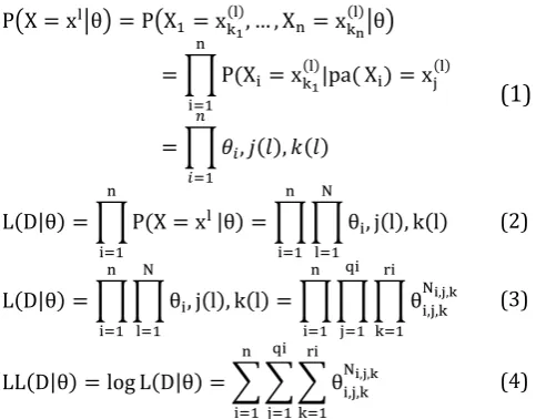
The conditional likelihood of this feature is computed by (1) and the density probability of the set of data D is

computed by (2). Since occurs whenever

and , (3) is deducted from (2), then the logarithmic notation of (3) gives (4).

( | ) ( | )

∏

(1)

∏

∏ ∏

(2)

∏ ∏ ∏ ∏ ∏

(3)

∑ ∑ ∑

(4)

Since [6] demonstrates that (4) formula can be simplified to (5), the Maximum Likelihood (ML) approach used in this paper is expressed by (6).

̂

∑

{ }

₍₅₎

̂( | ) ̂

∑ (6)

With being the number of features in the database

whose variable is in the state and parents are in the

configuration .

This classifier was improved by Naive Bayes to handle an arbitrary number of independent variables by constructing the posterior probability for the feature

given a set of variables, { } among a set

of possible outcomes { } by (7). Assuming

that the variables are statistically independent, the likelihood is decomposed to a product of terms in (8). Then from (8) the estimation computed by (9).

( ) ( | )

₍₇₎

∏ ( | )

(8)

( | ) ( ) ∏ ( | )

(9)

Where:

- ( ): Posterior probability of class

membership.

- ( | ) : Likelihood which is the

probability of the predicator given class.

- : class prior probability

Using (9), any new case X can be labeled by a class level with the highest posterior probability. Then after normalization, the decision distribution is :

√

( ( )

)

(10)

Where :

4. PROPOSED COMPUTATIONAL MODEL

[image:2.595.36.278.196.385.2]

The proposed computational protocol sketched in Figure 1, uses the following steps: (a) getting data from sensors (b) split training set from test data (c) learning/training the model (d) predict class using Naive Bayes model.

Figure 1: Naïve Bayes protocol for state estimation

A. Collecting data from sensors

During this step, the system collects data from a given number of sensors. Each sensor can be in one of the three states: low, adequate or high. Each sensor is assumed to be independent in terms of data types and collecting rate [14] [15]. The example provided in Table 1 gives the ranges for the training system of three sensors.

Table 1. Adequate range values for the system C.

Sensor S1 S2 S3

Values

B. Learning & training the model

The proposed model is “study on intelligent” say it was trained from data collected from sensors [15]. Hence, the state of the system depends on values provided by

Training data

Test data Posterior

probability Sensors

data capturing g

[image:2.595.314.539.351.498.2]

(3)

International Research Journal of Engineering and Technology (IRJET) e-ISSN: 2395-0056

© 2019, IRJET | Impact Factor value: 7.211 | ISO 9001:2008 Certified Journal

| Page 1801

different sensors: at time t, Ct depends on the state of S1t,

S2t, S3t, Snt. From example (Table 1), the System State

had 27 different probable classes. Each class is composed by 3 different states provide by the 3 sensors. The class C1can be represented by: S1low, S2adequate, S3high, meaning that at a given time t, sensor 1 sent a value lower than 16, sensor 2 sent a value between 20 and 25 and sensor 3 sent a value higher than 120. The learning process used it this paper can be summarized by algorithm 1 as follow:

Algorithm 1: Training process

Input: K (Training set)

For each class c in K do

Compute mean(k) and std(k)

End for

Output: mean, std

During the training stage, the mean and standard deviation values of the features for each class were computed.

C. Classification

Assuming that system parameters are distributed according to the Gaussian density, two parameters were

computed. First the parent node without parents . It

probability is the frequency of the class in the

training database. Since all the classes have the same probability at this stage:

( )

( ) ∑ ( )

∑ ( )

(11)

Where:

: The size of the database

( ): The number of observation belonging to the class

Second, the probability of the children nodes were computed by using the Normal law in conditional

probability of node considering the parent (12)

then combine the different values computed in the

previous step (13). in (13) being constant

hence easy to compute, (13) was rewritten as (14).

(12)

( | ) ( | )

(13)

( | )

( ) ( | ) ( | ) ( | )

(14)

D. Decision

The proposed Bayesian classifier (Algorithm 2) is a probabilistic model based on the Bayes rule [17] in

which each element ) is associated to a

class with a maximum a posteriori.

( | )

( )

( | ) ( | ) ( | )

(15)

Algorithm 2: Testing

Input: k(Learned features)

For each class li do

Calculate P(li|k)

End for

Output: { }(estimated

class)

The probabilities for the objective existing in each class are computed and the highest is chosen as the estimated class.

5. SIMULATION RESULTS

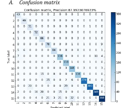
The proposed computational model was evaluated and its goodness was tested using the following evaluation parameters: accuracy, precision, recall, f1 score drawn from a confusion matrix. Furthermore, imbalanced data set results were compared to balanced data set results

[image:3.595.323.543.164.300.2]

A. Confusion matrix

Figure 2. Confusion matrix for imbalanced data set

[image:3.595.318.551.462.652.2]

(4)

International Research Journal of Engineering and Technology (IRJET) e-ISSN: 2395-0056

© 2019, IRJET | Impact Factor value: 7.211 | ISO 9001:2008 Certified Journal

| Page 1802

Figure 3. Confusion matrix with balanced data sent.

Comparative Accuracy

After varying the percentage of the learning set and the test set, we create 9 different set of data. Figure 3 show the relationship between the size of the learning set and the test set.

(a)

(b)

Figure 4: Relation between the size of the learning set and accuracy. (a) Imbalance data set (b) Balanced data set.

[image:4.595.56.258.76.251.2]

Better result are obtained when the size of the training set ranges between 40 to 65 % as shown in (a) and (b) in Figure 4. On the other hand taking the same number of data for each class in the training set (balanced data set) can improve the accuracy of the system from 87.3% to

96.33%. Accuracy is misled by the class with high support, thus reducing the overall accuracy as shown in (a).

Precision, recall, f1-score

(a)

[image:4.595.311.566.146.433.2]

(b)

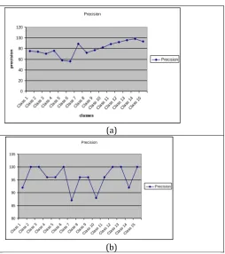
[image:4.595.52.264.361.698.2]

Figure 5: Precision (a) Precision for imbalance data set (b) Precision for balanced data set.

Figure 5 shows that the balanced data set achieves high precision than the imbalance data set, reaching 6 times a precision of 100%, on the other hand, the highest precision for classes in the imbalance data set reached hardly reached 100%. Figure 5 represents the sensitivity of balanced and imbalance data set.

In term of sensitivity, the balanced data set, produce a higher rate of sensitivity than the imbalance data set. F1-score conveys the balance between the precision and the recall, when dealing with imbalance classes, classification alone cannot be trusted to select a well performing model. Figure 8, shows the relationship between precision, recall and f1-score.

Accuracy

70 75 80 85 90 95 100

10% 20% 30% 40% 50% 60% 70% 80% 90%

Training set

A

c

ura

c

y

%

Accuracy

Precision

0 20 40 60 80 100 120

Class 1

Class 2

Class 3 Class

4 Class

5 Class

6 Class

7 Class

8 Class

9 Cla ss 1

0 Cla ss 1

1 Cla ss 1

2 Cla ss 1

3 Cla

ss 1 4 Cla ss 1

5

classes

pre

c

is

ion

Precision

80 85 90 95 100 105

Cla ss 1

Cla ss 2

Cla ss 3

Cla ss 4

Cla ss 5

Cla ss 6

Cla ss 7

Cla ss 8

Cla ss 9

Cla ss 1

0 Cla

ss 1 1 Cla

ss 1 2 Cla

ss 1 3 Cla ss 1

4 Cla

ss 1 5

Precision

Accuracy

85 85.5 86 86.5 87 87.5

10% 20% 30% 40% 50% 60% 70% 80% 90%

Training set

A

c

ura

c

y

%

(5)

International Research Journal of Engineering and Technology (IRJET) e-ISSN: 2395-0056

© 2019, IRJET | Impact Factor value: 7.211 | ISO 9001:2008 Certified Journal

| Page 1803

(a)

[image:5.595.30.558.22.809.2]

(b)

Figure 6: Recall (a) Precision for imbalance data set (b) Precision for balanced data set.

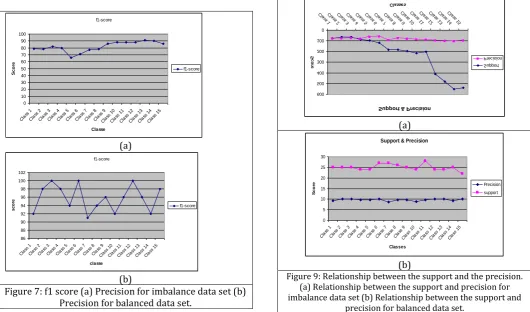
The support of the class in the training set has a positive impact on the precision of the class, especially when we have imbalance class in the training set. Figure 7 shows the relationship between the support and the precision.

(a)

(b)

Figure 7: f1 score (a) Precision for imbalance data set (b) Precision for balanced data set.

(a)

[image:5.595.322.547.50.358.2]

(b)

Figure 8: Precision (a) Precision for imbalance data set (b) Precision for balanced data set.

For imbalance class in the training set, the support of a class has a positive impact on the precision of the class; however, classes with a very high accuracy can create an accuracy paradox problem by predicting the value of the majority class for all predictions and achieve high classification accuracy.

(a)

(b)

Figure 9: Relationship between the support and the precision. (a) Relationship between the support and precision for imbalance data set (b) Relationship between the support and

precision for balanced data set. Recall 0 20 40 60 80 100 120 Cla ss 1

Cla ss 2

Cla ss 3

Cla ss 4

Cla ss 5

Cla ss 6

Cla ss 7

Cla ss 8

Cla ss 9

Cla ss 1

0 Cla

ss 1 1 Cla ss 1

2 Cla

ss 1 3 Cla

ss 1 4 Cla ss 1

5 classe S c ore Recall Recall 88 90 92 94 96 98 100 102 Cla ss 1

Cla ss 2

Cla ss 3

Cla ss 4

Cla ss 5

Cla ss 6

Cla ss 7

Cla ss 8

Cla ss 9

Cla ss 1

0 Cla

ss 1 1 Cla

ss 1 2 Cla

ss 1 3 Cla

ss 1 4 Cla ss 1

5 Classe S c ore Recall f1-score 0 10 20 30 40 50 60 70 80 90 100 Cla ss 1

Cla ss 2

Cla ss 3

Cla ss 4

Cla ss 5

Cla ss 6

Cla ss 7

Cla ss 8

Cla ss 9

Cla ss 1

0 Cla ss 1

1 Cla ss 1

2 Cla ss 1

3 Cla ss 1

4 Cla ss 1

5 Classe S c ore f1-score f1-score 86 88 90 92 94 96 98 100 102 Cla ss 1

Cla ss 2

Cla ss 3

Cla ss 4

Cla ss 5

Cla ss 6

Cla ss 7

Cla ss 8

Cla ss 9

Cla ss 1

0 Cla ss 1

1 Cla

ss 1 2 Cla ss 1

3 Cla ss 1

4 Cla ss 1

5 classe s c ore f1-score Precision,Recall,f1-score 0 20 40 60 80 100 120

Class 1 Class

2 Class

3 Class

4 Class

5 Class

6 Class

7 Class

8 Class

9

Class 10 Class

11 Class

12 Class

13 Class

14 Class

15 Classes S c o re i n % Precision Recall f1-score

Precision, recall, f1-score

80 85 90 95 100 105 Cla ss 1

Cla ss 2

Cla ss 3

Cla ss 4

Cla ss 5

Cla ss 6

Cla ss 7

Cla ss 8

Cla ss 9

Class 10

Class 11 Class

12 Class

13 Class

14 Class

15 score % C la s s e s Precision Recall f1-score

Support & Precision 0 100 200 300 400 500 600 C_la ss₁

C_la ss₂

C_la ss₃

C_la ss₄

C_la ss₅

C_la ss₆

C_la ss₇

C_la ss₈

C_la ss₉

C la ss 10 C la ss 11 C la ss 12 C la ss 13 C la ss 14 C la ss 15 Classes S c ore Support Precision

Support & Precision

0 5 10 15 20 25 30 Cla ss 1

Cla ss 2

Cla ss 3

Cla ss 4

Cla ss 5

Cla ss 6

Cla ss 7

Cla ss 8

Cla ss 9

Cla ss 1

0 Cla

ss 1 1 Cla

ss 1 2 Cla

ss 1 3 Cla

ss 1 4 Cla

[image:5.595.29.289.53.358.2] [image:5.595.32.563.448.760.2]

(6)

International Research Journal of Engineering and Technology (IRJET) e-ISSN: 2395-0056

| Page 1804

6.

DISCUSSIONS AND CONCLUSION

A novel multi-sensor system smart control model based on Bayesian data was proposed. The proposed algorithm is able to predict the state of a system taking into account the actual and the anterior data collected from different types of sensors. For test seek, a three sensors system (sol temperature, air temperature, and moisture) was set and the algorithm performance was measured. Simulation tests have proved that the proposed algorithm can predict at an overall rate of more than 96% the actual state of the system.

Since the trained and proposed model is “study on intelligent”, the algorithm reduces the reliance on experts. It is a “previous system data” dependent model. This means that any non-expert can train and use the system. A few expertise is only required during the training step of the system. However, a real life customizable implementation of the proposed algorithm is needed.

7. REFERENCES

[1] H. Mitchell, Multi-Sensor Data Fusion: An Introduction, Berlin: Springer.

[2] D. Hall and J. Llinas, Handbook of Multisensor Data Fusion, New York, 2001.

[3] M. Wang and all, "City Data Fusion: Sensor Data Fusion in the Internet of Things," International Journal of Distributed Systems and Technologies, June2015.

[4] F. Aiam and All, "Data Fusion and IoT for Smart Ubiquitous Environments: A Survey. ,," IEEE. [5] B. Yang, X. Liu and X. Z. Y. Li, "Stochastic

Blocmodeling and variational Bayes Learning for Signed Network Analysis," in IEEE Transactions on Knowledge and Data Engineering, May 2017. [6] D. Hall and A. Garga, "Pitfalls in data fusion(and how

to avoid them)," Proceedings of the Second International Conference on Information Fusion (Fusion ’99), vol. 1, pp. 429-439, 1999.

[7] H. Holzapfel, K. Nickel and R. Stiefelhagen, "Implementation and evaluation of a constraint-based multimodal fusion system for speech and 3D pointing gestures," Proc. 6th Int. Conference Multimodal interfaces- ICMI ’04, p. 175, 2004. [8] F. Shen and R. Yan, "A Thermostatic Control

Strategy Based on Multi-sensor Data Fusion and Fuzzy PID Method," in Tenth Internation Conference on Sensing Technology, 2016.

[9] J. He, S. Bai and X. Wang, "An Unobtrusive Fall Detection and Alerting System Based on Kalman Filter and Bayes Network Classifier," Sensors 2017, vol. 14, p. 1393, 2017.

[10] R. Mahler, Unified Bayes Multi target Fusion of

Ambigous Data Sources, Boston, USA: Kimasi, 2003. [11] A. Ashari, I. Paryudi and A. Tjoa, "Performance Comparison between Naive Bayes, Decision tree and K-Nearest Neighbor in Searching Alternative Design in an Energy Simulation Too," IJACSA, International Journal of Advanced Computer Science and Applications, vol. IV, no. 11, 2013. [12] X. Meng, G. Bai, X. Shu and D. Bao, "A study of

intelligent fault diagnosis in engine room by Bayes method;, 2002.," IEEE; Intelligent Control and Automation. Proceedings of the 4th World Congress, 2002.

[13] G. Myburgh and A. V. Niekerk, "Impact of training set size on object-based land cover classification: A Comparison of three classifiers," International Journal of Applied Geospacial Research, vol. V, no. 3, pp. 49-67, July 2014.

[14] D. J. Hand and K. Yu, "Idiot’s bayes : Not so stupid after all?," International statistical Review, 2001. [15] M. Godec, C. Leistner, A. Saffari and H. Bischof,

"On-Line Random Naïve Bayes for Tracking," IEEE,

Pattern Recognition (ICPR), 2010 20th

International Conference, 2010.

BIOGRAPHIES

Mumbere Muyisa Forrest is a MSc holder in Information Technology and a Lecturer of IT courses at Université Adventiste de Lukanga and Institut de Commerce de Beni in RDC. He is currently preparing his PhD in Software Engineering in School of Software at Central South University, Changsha 410000, China.

Dr MASIVI is a Computer Science PhD holder from University of the Philippines Los Banos. He is

currently Associate Professor

lecturing IT and Computer Science courses at Rusangu University (Zambia) and ISP/Muhangi (RDC).

Kasereka Masivi Samuel is a MSc holder in Information Technology and a Lecturer of courses at Université Adventiste de Lukanga and Université de Bunia in DRC. He is currently preparing his PhD in Computer Science at Invertis University, India.