147
Considering chain to chain competition in forward and reverse
logistics of a dynamic and integrated supply chain network design
problem
Arash Nobari
1*, Amirsaman Kheirkhah
1, Maryam Esmaeili
21
Industrial Engineering Department, Faculty of Engineering, Bu-Ali Sina University, Hamedan, Iran
2
Industrial Engineering Department, Faculty of Engineering, Al-Zahra University, Tehran, Iran
[email protected], [email protected], [email protected]
Abstract
In this paper, a bi-objective model is presented for dynamic and integrated network design of a new entrant competitive closed-loop supply chain. To consider dynamism and integration in the network design problem, multiple long-term periods are regarded during planning horizon, so that each long-term period includes several short-term periods. Furthermore, a chain to chain competition between two rival supply chains is considered in both forward and reverse logistics. In the forward logistics, the rivals have to compete on the selling price, while in the reverse logistics, the supply chains compete on incentive buying price to achieve more market share. To solve the competitive stage of the proposed model, a game theoretic approach, which determines the selling and incentive buying prices of forward and reverse logistics, is used. Based on the competitive stage’s outputs, the resulted dynamic and integrated network design stage is solved using a Pareto-based multi-objective imperialist competitive algorithm. Finally, to evaluate efficiency of the proposed model and solution approach, a numerical study is implemented.
Keywords: Supply chain network design, chain to chain competition,
forward/reverse logistics game theoretic approach, Pareto-based meta-heuristic algorithm.
1- Introduction
Nowadays, one of the most important strategic decisions of supply chain management (SCM), which has a significant influence on the future performance of supply chains, is the supply chain network design (SCND) problem. The SCND problem aims to find an efficient structure for a supply chain, so that the flow of good and data among different echelons of supply chain can be facilitated (Simchi-Levi, Kaminsky and Simchi-Levi, 1999). In the literature of SCND problem, many researchers concentrated only on strategic network design decisions, regardless of tactical and operational performance of supply chains. In contrast, reciprocal interaction among infrastructure of a supply chain and future tactical and operational performance of supply chain made some researchers consider short-term decisions integrality, beside strategic supply chain network design problem (Melo, Nickel and Saldanha-da-Gama, 2009; Ghavamifar, Sabouhi and Makui, 2018).
*Corresponding author
ISSN: 1735-8272, Copyright c 2019 JISE. All rights reserved
Journal of Industrial and Systems Engineering
Vol. 12, No. 1, pp. 147-166 Winter (January) 2019
148
In this manner, a comprehensive survey about the SCND problem has been studied by Shen (2007). According to the expensive nature of strategic decisions, most researchers studied the SCND problem as an unchangeable single-period problem (Fattahi et al., 2015). On the other hand, some researchers investigated the dynamic SCND problem in which the structure-related decisions can be changed during multiple strategic periods (Mota et al., 2014; Govindan, Jafarian and Nourbakhsh, 2015; Keyvanshokooh et al., 2013; Dubey, Gunasekaran and Childe, 2015; Rahmani, and Mahoodian, 2015). There are a few researches in which several strategic periods and several tactical periods are considered, simultaneously (Badri, Bashiri and Hejazi, 2013).
In the recent years, reducing operational cost, waste management, environmental legislations, government pressures, and etc. made supply chains to consider designing reverse logistics in their networks as well as forward logistic (Kamali et al., 2014; Shi, Zhang and Sha, 2011a; Shi, Zhang and Sha, 2011b; Pishvaee and Razmi, 2012; Soleimani et al., 2017; Kaya and Urek, 2015; Accorsi et al., 2015; Nobari, Kheirkhah and Esmaeili, 2016). In reverse logistics, companies focus on returning products from customer zones and preparing them for reusing. Govindan, Soleimani and Kannan (2015) presented a comprehensive study about reverse logistics and closed-loop supply chains. In this paper, a closed-loop supply chain network design (CLSCND) problem is studied.
In spite of the growing competitive environment in which different supply chains with similar business act in the same markets, most researches evaluate the SCND problem in an uncompetitive and monopoly environment (Fallah, Eskandari and Pishvaee, 2015). Todays, different supply chains can be found in each market and these supply chains have to compete with each other to achieve their goals (Dubey, Gunasekaran and Childe, 2015). Through the studies by which the competition in SCND problem is considered, most of researchers studied the competition within a supply chain and among its different firms, while globalization of services change the inner competition of supply chains into chain to chain form (Zanjirani Farahani et al., 2014; Yazdi and Honarvar, 2015; Makui and Ghavamifar, 2016; Bilir, Onsel Ekici and Ulengin, 2017; Fahimi, Seyedhosseini, and Makui, 2017a; Hosseini-Motlagh, Nematollahi and Nouri, 2018). In a chain to chain competition, different firms of a supply chain cooperate with each other to reach a competitive advantage with respect to the other supply chains. There are a few researches which have studied the competitive SCND problem (Nagurney, Dong and Zhang, 2002; Rezapour, S., and Zanjirani Farahani, 2010; Rezapour et al., 2011; Rezapour, Zanjirani Farahani and Drezner, 2011; Hafezalkotob et al., 2014; Nobari, Kheirkhah and Esmaeili, 2018). A comprehensive study about competitive SCND problem has been provided by Zanjirani Farahani et al., (2014). Most researches in the literature of competitive SCND problem, have focused on competition in forward logistics (Hafezalkotob et al., 2014; Yousefi Yegane, Nakhai Kamalabadi and Farughi, 2016; Saghaeeian and Ramezanian, 2018). A few researches considered the competitive aspects in both forward and reverse logistics (Fallah et al., 2015). In a competitive CLSCND problem, competition in both forward and reverse logistics is regarded.
It is obvious that considering different aspects of the SCND design problem can lead to more realistic and realible results. Accordingly, in this paper, a novel competitive dynamic and integrated supply chain network design problem is presented. In this manner, a multi-objective model is proposed for network design of a new entrant closed-loop supply chain which has to compete with a rival, in both forward and reverse logistics. The main contributions of this paper are as follow:
Dynamic network design of competitive supply chain, so that the structure of the new entrant supply
chain can be changed during several strategic periods.
Consideration of chain to chain competition in both forward and reverse logistics of supply chain.
Integration of short-term decisions with strategic long-term network design decisions.
Presenting an efficient Pareto-based multi-objective meta-heuristic approach, empowered by game
theory, to solve the proposed model.
The rest of this paper is organized as follows: Section 2 includes definition of the proposed competitive CLSCND problem for which a multi-objective model is formulated. The solution approach is described in
149
section 3. Some numerical examples are analysed for the proposed model and the solution approach in section 4. Finally, the conclusion and future research suggestions are given.
2- Problem definition
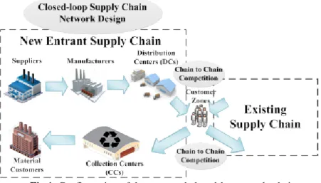
In this paper, integrated and dynamic network design of a new entrant supply chain, which acts in a competitive environment, is considered. The forward logistics of this supply chain includes several suppliers, manufacturers, and distribution centers (DC) and in the reverse logistics there are several collection centers (CC) and material customers. The manufacturers produce different products using raw materials which are provided by the suppliers and then, send the final products to the DCs. Finally, the distribution centers sell the products in multiple customer zones. In the reverse logistics, the CCs collect the used products from customer zones and sell them to raw material customers. The configuration of this closed-loop supply chain is shown in figure 1.
Fig 1. Configuration of the proposed closed-loop supply chain
It is assumed that there is an existing supply chain with a predefined structure which produces the substitutable products and sells them in the customer zones. Hence, the entrant supply chain has to compete with this existing supply chain in two ways:
In the forward logistics, both supply chains compete with each other to achieve more market
share in each customer zone.
In the reverse logistics, each supply chain aims to collect more used products with respect to the
other supply chain.
The competition among these supply chains will be explained more in section 2.3.
It is also supposed that the planning horizon consists of multiple strategic periods so that each strategic period includes several tactical periods. This assumption is considered to integrate tactical decisions with strategic ones. Moreover, it is assumed that the supply chain can extend the capacities of manufacturers during the planning horizon. For each strategic period, there is a defined budget which can be assigned to open new facilities and extend the capacities of current facilities, dynamically.
The aim of the proposed competitive SCND problem is finding the best structure and capacity options for the new entrant closed-loop supply chain with respect to existing supply chain, so that both economic and environmental concerns can be achieved, simultaneously. In each strategic period, the long-term decisions including opening new facilities and extending the capacities of manufacturers are determined, while the short-term decisions would are defined in each tactical period.
The other assumptions of the proposed model are as follow:
The potential locations for facilities are determined.
The opened facilities in each strategic period cannot be closed during the next strategic periods.
150
The maximum capacity of each facility is known.
The demand function of each customer zone depends linearly only on the selling prices of rivals.
The accusation function of the used products depends linearly only on the incentive buying prices
of both competitive supply chains.
Shortages can occur in form of the lost sales.
The budget assigned to each strategic period is determined
All the parameters are deterministic.
2-1- Notations
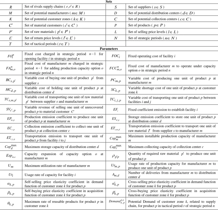
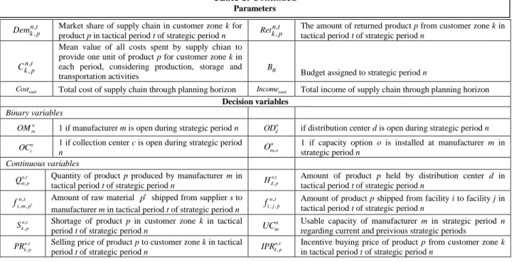
All the notations, parameters, and decision variables used in the proposed mathematical mode are stated in table 1.
Table 1. Notations of proposed model
Sets
R Set of rivals supply chains ( ,r rR) S Set of suppliers (sS)
M Set of potential manufacturers (mM) D Set of potential distribution centers (dD)
K Set of potential customer zones (kK) C Set of potential collection centers (cC) C Set of material customers (cC) P Set of products (pP)
P Set of raw materials (pP) L Set of selling price levels (lL)
L Set of return price levels (lL) N Set of strategic periods (nN)
T Set of tactical periods (tT)
Parameters n
i
FO Fixed cost charged in strategic period n1 for
opening facility i in strategic period n FOCi Fixed operating cost of facility i ,
n m o
FA
Fixed cost of manufacturer m charged in strategic period n1 for adding production capacity option o
in strategic period n
,
n m o
FCC Fixed cost of manufacturer m to operate under capacity
option o in strategic period n
,
s p
BC Variable cost of buying one unit of product p from
supplier s PCm p,
Variable cost of producing one unit of product p at manufacturer m
,
d p
HC Variable cost of holding one unit of product p at
distribution center d SCk p,
Variable shortage cost of one unit of product p at customer zone k
, ,
s m p
TC Variable cost of transporting one unit of raw material
p between supplier s and manufacturer m TCi j p, ,
Variable cost of transporting one unit of product p between facilities i and j
,
c p
SV Variable revenue of selling one unit of unrecovered product p to material customer C EFi Fixed coefficient emission to establish facility i
,
m p
EP Production emission coefficient to produce one unit
of product p at manufacturer m ESd p,
Storage emission coefficient to store one unit of product p
at distribution center d ,
c p
EC Collection emission coefficient to collect one unit of
product p at collection center c ETs m p, , Transportation emission coefficient to transport one unit of raw material l from supplier s to manufacturer m , ,
i j p
ET Transportation emission to transport one unit of
product p from facility i to j
max
m
Cap Maximum installable production capacity of manufacturer m
max
d
Cap Maximum storage capacity of distribution center d Capmaxc Maximum collecting capacity of collection center c
,
m o
Exp Capacity expansion of capacity option o at
manufacturer m p p
Quantity of required raw material p to produce one unit of product p
m
U Maximum utilization rate of manufacturer m Urm p, Usage rate of production capacity for manufacturer m to
produce one unit of product p
i
Ur Usage rate of capacity for facility i Am d, Number of deliveries from manufacturer center d m to distribution ,
k p
Self-selling price elasticity coefficient in demand function of customer zone k for product p k p,
Cross-selling price elasticity coefficient in demand function of customer zone k for product p
,
k p
Self-buying price elasticity coefficient in acquisition function of customer zone k for product p k p,
Cross-buying price elasticity coefficient in acquisition function of customer zone k for product p
,
k p
Maximum rate of reusable products for product p in customer zone k
, , n t k p
Demand Potential Demand of customer zone k, related to supply chain, for product p in tactical period t of strategic period n
151
, ,
n t k p
Dem Market share of supply chain in customer zone k for
product p in tactical period t of strategic period n
, ,
n t k p
Ret The amount of returned product p from customer zone k in tactical period t of strategic period n
, ,
n t k p
C
Mean value of all costs spent by supply chian to provide one unit of product p for customer zone k in each period, considering production, storage and transportation activities n
B
Budget assigned to strategic period n
total
Cost Total cost of supply chain through planning horizon Incometotal Total income of supply chain through planning horizon Decision variables
Binary variables
n m
OM 1 if manufacturer m is open during strategic period n n d
OD if distribution center d is open during strategic period n
n c
OC 1 if collection center c is open during strategic period
n ,
n m o
O 1 if capacity option o is installed at manufacturer m in
strategic period n Continuous variables
, ,
n t m p
Q Quantity of product p produced by manufacturer m in
tactical period t of strategic period n
, ,
n t d p
H Amount of product p held by distribution center d in
tactical period t of strategic period n
, , , n t s m p
f Amount of raw material p shipped from supplier s to
manufacturer m in tactical period t of strategic period n
, , , n t i j p
f Amount of product p shipped from facility i to facility j in
tactical period t of strategic period n
, ,
n t k p
S Shortage of product p in customer zone k in tactical
period t of strategic period n
n m
UC Usable capacity of manufacturer m in strategic period n
regarding current and preivious strategic periods
, ,
n t k p
PR Selling price of product p to customer zone k in tactical
period t of strategic period n
, ,
n t k p
IPR Incentive buying price of product p from customer zone k
in tactical period t of strategic period n
2-2- Model formulation
In this sub-section, the objective functions of the multi-objective model are described, and then the constraints are discussed.
2-2-1- Objective functions (OF)
Maximizing total profit of supply chain (equation 1), which is the difference between total income (equation 1a) and total cost (equation 1b) of supply chain, is the first objective function of proposed model.
1 total total
Max OF Income Cost (1)
, , ,
, , , , , , ,
, 0 , 0
n t n t n t
total k p d k p c c p c c p
n N n t T d D k K p P n N n t T c C c C p P
Income PR f SV f
(1a) , ,, 0 , 0 , 0 , 0 0
, , ,
, , , , , , ,
, 0 , 0
n n n n n n n n
Var m m d d c c m o m o
n N n m M n N n d D n N n c C n N n t T o O n n
n t n t n t
s p s m p m p m p m p d p
n N n t T s S m M p P n N n t T m M p P
Cost FOC OM FOC OD FOC OC FCC O
BC f PC Q HC H
, , , , , 0 , , , , , , , , , , , , , ,, 0 , 0 , 0
, ,
1 2
n t m d p
m d
n N n t T d D p P m M
n t n t n t n t
k p k p l k p k c p s m p s m p
n N n t T k K p P l L n N n t T k K c C p P n N n t T s S m M p P
m d p
n t T m M d D p P
f A
SC S IPR f TC f
TC
, , , , , , , , , , , , ,, 0 , 0 , 0
n t n t n t
m d p d k p d k p k c p k c p
N n n N n t T d D k K p P n N n t T s S m M p P
f TC f TC f
(1b)
Recently, green manufacturing has been attended widely in the SCND problem (Ma et al., 2018; Hosseini-Motlagh, Laari, Toyli and Ojala, 2017; Nematollahi and Nouri, 2018). In this manner, life cycle analysis (LCA) method, by which the released waste is quantified through the product life cycle, helps firms to consider environmental performance (Liu, Qiu and Chen, 2014; Rabbani, Keshvarparast and Farrokhi-Asl, 2016). Hence, minimizing the amount of emissions arising from establishment, operation and transportation of the facilities is regarded as the second objective function of the proposed model which is stated by equation 2.
Table 1. Continued
152
2
, ,
, , , ,
, 0 , 0
, , , , , , , , , , 0 +
M D C
T
NT NT NT
m m d d c c
m d c
n t n
M P T D
t
m p m p d p d p
n N n t m p n N n t d p
n t n t
c p k c p s m p s m p
n N n t
P
T k K cC p P
Min OF EF OM EF OM EF OC
EP Q ES H
EC f ET f
, 0 , , , , , , , , , ,, 0 , 0
, ,
, , , , , , , ,
, 0
+
n N n t s m p
n t n t
m d p m d p d k p d k p
n N n t m d p n N n t d k p
n t n t
k c p k c p c c p c c p
n N n
T S M P
T M D P T D K P
T K C P
t k c p p
ET f ET f
ET f ET f
, 0n N n
t T c C cC P(2)
2-2-2- Constraints
, ,
, , , , , , 0,
n t n t
s m p S
p p m p
s pP
f Q m p n t
(3), ,
, , , , , 0,
n t n t
m p m d p
d D
Q f m p n t
(4), 1 , , ,
, , , , , , , , , 1
n t n t n t n t
d p m d p d p d k
k K p M
m
H f H f d p n t
(5)
1, , , ,
, , , , , , , , , 1
n T n t n t n t
d p m d p d p d k p
mN k K
H f H f d p n t
(6)
, ,
, , , , , , 0,
n t n t
k c p c c
K C
k c
p
f f c p n t
(7), , ,
, , , , 0,
n t n t n t
d k k p D
k p d
f S Dem p n t
(8), ,
, , , ,
C D
n t n t
k c p d k p
c d
f f
(9)1
, 0
n n
m m
OM OM m n (10)
1
, 0
n n
d d
OD OD d n (11)
1
, 0
n n
c c
OC OC c n (12)
1 1 1 1 1 1 1 1
, ,
n n n n n n
m m m d m m
m d
n n n n n n
c m m m o m o
c
M D
C mM oO
FO OM OM FO OD OD
FO OC OC FA O B
(13), , 0
O
n n
m o m
o
O OM m n
(14), ,
,
, 0
O
n n
m m o m o
n n n N o
UC Exp O m n
(15),
, , , 0,
n t n
m p P
m p p m m
Ur Q U UC m n t
(16)max
, 0
n n
m m m
UC Cap OM m n (17)
, , , , max , , 1 , 0, 2 n t m d p
n t n
p d p p d d
m d
p m M p P
f
Ur H Ur OD Cap d n t A
153
, max
, , , 0,
n t n
k c p c c
k K p P
f OC Cap c n t
(19)
,
, , , , , , ,
, , , , , , , , , ,
, , , 0,1
, , , , , , , 0
n n n n
m d c m o
n t n t n t n t n t n t n t
m p d p s m p i j p k p l k p k p n
OM OD OC O
Q H f f S PR IPR UB
(20)
Equation 3 confirms that each manufacturer buys sufficient raw material from suppliers. Equation 4 indicates all the products are transported to the distribution centers in each period. Equation 5 and equation 6 assure that in each tactical period, the sum of input products and stored products of the previous tactical period equals to the output products plus the amount of products stored in current tactical period. Equation 7 indicates each collection center sells all the products collected from the customer zones. Equation 8 states that in each period, the sum of delivered products to customer zones and shortage equals to the corresponding market share in that period. Equation 9 indicates the amount of returned products in each period which is less than provided market share. Equations 10 and 12 confirms that open facilities cannot be closed in next periods. Equation 13 limits the fixed cost of opening facilities to the assigned budget of strategic periods. Equation 14 assures that only one capacity option can be activated in each strategic period. Equation 15 calculates the usable capacities for each manufacturer based on current and previous strategic periods. Equation 16 confirms that in each tactical period, the employed capacity in each manufacturer is less than the maximum utilization rate. Equation 17 limits the overall capacity manufacturers. Equation 18 and equation 19 express the capacity limitation of DCs and CCs, respectively. Finally, equation 20 indicates the decision variables.
2-3- Competition of supply chain
In this sub-section, the competitions among the new entrant and existing supply chains in forward and reverse logistics are formulated.
The demand in competitive markets depends on performance of all competitors. In this paper, the linear price-sensitive demand function, which is a known price-sensitive demand function, is considered to formulate the demand function of each customer zone for supply chains (Fattahi et al., 2015). Equation 21
indicates the market share of supply chain r with respect to both rival supply chains
, , , ,
, , , , , , , , , , , ,
n t n t n t n t
r k p r k p r k p r k p r k p r k p
Dem Demand
PR
PR (21)Where ,
, ,
n t r k p
PR and ,
, ,
n t r k p
PR indicates the selling price of supply chain r and its rival (r), respectively.
Furthermore, it is also assumed that there is a competition among supply chains in returning reusable products. In the recent years, competition in reverse logistics is regarded in some researches (Wu and Zhou, 2017). Hence, a simple linear price-sensitive acquisition function is considered to formulate the relationship among the amount of returned products and buying prices of supply chains which can be formulated as equation 22.
, , , ,
, , , , , , , , , , , , , ,
Re n t n t n t n t
r k p r k p r k p r k p r k p r k p r k p
t Demand IPR IPR (22)
Where ,
, ,
n t r k p
IPR and ,
, ,
n t r k p
IPR are incentive buying price of supply chain r and its rival (r), respectively.
Indeed, equation 22 indicates the market share of entrant supply chain in returning used products.
Based on selling products in forward logistics and selling returned products in reverse logistics, the
profit function of supply chain r, in each customer zone and in each tactical period can be formulated as
equation 23.
, , , , , , ,
, , , , , , , , , , , Re , ,
n t n t n t n t n t n t n t
r k p PRr k p Cr k p Demr k p SVc p IPRr k p tr k p
(23)
In order to solve the model, the competitive part of the proposed model is solved first. Then, the defined selling and buying prices are substituted in the formulated model. The solution approach is more explained in section 4.
154
3- Solution approach
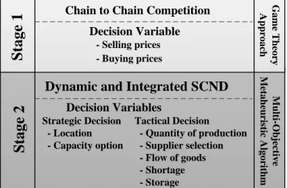
In this paper, the solution approach contains two steps. First, the game theory approach is used to solve the competitive pricing problem, as discussed in subsection 3-1. The outputs of this step (selling and incentive buying prices) are substituted in the proposed model, and then a meta-heuristic algorithm is used to solve the achieved model, as presented in subsection 3-2. Figure 2 indicates two steps of the solution approach.
Chain to Chain Competition Decision Variable - Selling prices - Buying prices
Dynamic and Integrated SCND
Decision Variables
Strategic Decision Tactical Decision
- Location - Quantity of production - Capacity option - Supplier selection
- Flow of goods - Shortage - Storage G a m e T h eo ry A p p ro a ch
S
ta
g
e
1
S
ta
g
e
2
M u lt i-O b je ct iv e M et a h eu ri st ic A lg o ri th mFig 2. Steps of solution approach
3-1- Competitive step
As mentioned in section 2-3, simultaneous competitions in both forward and reverse logistics exist among the new entrant and existing supply chains. In fact, in each customer zone, both supply chains have to determine their selling and incentive buying prices with respect to the competitor supply chain. To solve these competitions, the game theory approach, by which the equilibrium values for selling prices and incentive buying prices are obtained, is used. Since in this type of competitions, players define their decisions simultaneously, Nash equilibrium can be achieved for the supply chains based on Fallah et al. (2015).
To find the optimum value of selling and incentive buying prices, the concavity of profit function of equation 23 is evaluated with respect to these competitive decision variables. So, the first and second order derivations of the profit function to selling and buying prices are calculated using equations 24 to 29. , , , , , , , , , , , , , , , , , , , , , , , , 2 n t
r k p n t n t n t n t
r k p r k p r k p r k p r k p r k p r k p
n t r k p
Demand PR PR C
PR
(24)
, , , , , , , , , , , , , , , , , , , , , , , , , 2 n t
r k p n t n t n t n t
r k p r k p r k p r k p r k p r k p r k p c p n t
r k p
IPR IPR Demand SV
IPR
(25)
2 , , , , , , 2 , , 2 n t r k p
r k p n t
r k p
PR
(26)
2 , , , , , , , , , 0 n t r k p
n t n t
r k p r k p
PR IPR
(27)
2 , , , , , , 2 , , 2 n t r k p
r k p n t
r k p
IPR
155 2 , , , , , , , , , 0 n t r k p
n t n t
r k p r k p
IPR PR
(29)
The Hessian matrix can be calculated using equation 30.
, ,
, ,
2 0
0 2
r k p
r k p
H
(31)
Based on equation 27, the Hessian matrix is definitely negative (det( )H 0). Hence, the profit function is
concave.
Accordingly, the optimal values of selling and incentive buying prices can be calculated by setting the first order partial derivations to zero, as formulated by equations 31 and 32.
, , , , , , , , , , , , , , , , , , , , , , , , 2 0 n t
r k p n t n t n t n t
r k p r k p r k p r k p r k p r k p r k p
n t r k p
Demand PR PR C
PR
(31)
, , , , , , , , , , , , , , , , , , , , , , , , , 2 0 n t
r k p n t n t n t n t
r k p r k p r k p r k p r k p r k p r k p c p n t
r k p
IPR IPR Demand SV
IPR
(32)
By solving these equations, the optimal values for selling and incentive buying prices are calculated using equations 33 and 34.
, , , *
n t r k p
PR
, , , ,
, , , , , , , , , , , , , , , , , ,
, , , , , , , ,
2 4
n t n t n t n t
r k p r k p r k p r k p r k p r k p r k p r k p r k p
r k p r k p r k p r k p
Demand Demand C C
(33) , , , , , , , , , , , , , , , , , , , , , , , , , , , , , , , , , , , , , 2 2 * 4
n t n t n t n t
r k p r k p c p r k p r k p c p r k p r k p r k p r k p r k p r k p n t
r k p
r k p r k p r k p r k p
SV SV Demand Demand
IPR
(34)
Now, the optimal values for selling and incentive buying prices which are calculated regarding the chain to chain competition should be substituted in the proposed model stated in equations 1 to 20.
3-2- Dynamic and integrated network design step
According to the optimal values, resulted in the competitive stage, a MINLP bi-objective model is achieved. Recently, the confliction among different goals of multi-objective problems, made many researchers use Pareto-based meta-heuristic algorithm to solve multi-objective models. In these types of
models, there are several objective functions including OF x( ) OF x1( ),...,OF xm( ) with respect to multiple
constraints such as g xi( )0 , i1,2,..., ,c xX, where x is the solution vector and X is the feasible
region. In a maximization form, the domination of solution a to solution b a b( , X) can be described as
follows:
1) f ai( ) f bi( ), i 1, 2, ...,m 2) i {1, 2, ..., }:m f ai( ) f bi( )
Pareto solutions (Pareto fronts) consist of solutions which cannot dominate each other. The goodness of these solutions can be evaluated by diversity and convergence of the solutions (Deb et al., 2002).
In this paper, in order to solve the proposed multi-objective model, a multi-objective imperialist competitive algorithm (MOICA) which is a Pareto-based meta-heuristic algorithm is used.
3-2-1- Multi-objective imperialist competitive algorithm
Imperialist competitive algorithm (ICA) is a meta-heuristic algorithm which is inspired by a social phenomenon, called imperialism. For the first time, Atashpaz-Gargari and Lucas (2007) introduced this algorithm. The capabilities of ICA in solving single-objective models encouraged many researchers to use
156
multi-objective version of ICA. MOICA which is a Pareto-based meta-heuristic algorithm is introduced by Enayatifar et al. (2013).
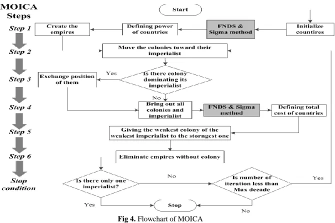
In this paper, MOICA is used to solve the multi-objective model. The steps of proposed MOICA are as follows:
- Step 1: Initializing the empires
In this step
N
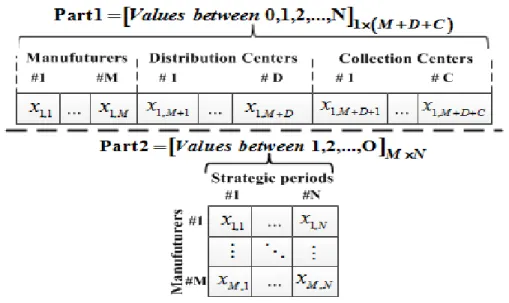
pop countries (number of population) are created, randomly. The solution representation forthe proposed model includes two parts, as shown in Figure 3:
Part 1: A vector with M+D+C cells (number of manufacturers, DCs, CCs). The value of each cell
includes a number between 0 to N, which indicates the strategic periods in which the related facility is
opened. Zero value indicates that the facility stays closed during the planning horizon.
Part 2: A MN matrix which determines the activated capacity option for manufacturers in each
strategic period.
In order to create the countries, the values of these vectors should be initialized for each country, and then based on these defined values, the other tactical decision variables for each solution are created, randomly.
Fig 3. Solution representation
Now, Nimp of most powerful created countries are selected as imperialists for whom the other remaining
countries are colonies. Number of colonies, assigned to each imperialist, is based on two following criteria which indicate the power of imperialist:
1- Rank of each country, which is based on the fast non-dominated sorting (FNDS) technique and
considers all the objective functions.
2- Merit of each country, compared to countries with the same rank, which is based on the crowding
distance criterion.
Based on Enayatifar et al. (2013), the power of each country is calculated using equation 35.
1 ( )
1 1
( ) ( ) ( ) 1
N C
D
n j j
j i
rank
Power OF n OF i Rank C D
(35)
Where D is the number of objective functions OF ij( ) is value of the jth objective function of country i and
( )
rank
N C is the number of countries in rank C.
157
n n col
NC round p N (36) Where
1
imp
n n N
i i
power p
power
, indicates the imperialists power ratio.
- Step 2: Moving of the colonies toward their imperialist
In this algorithm, it is assumed that the colonies, seized by imperialist, move gradually toward the position of their imperialist and a deviation might occur during this movement. The movement of each colony and its possible deviation can be calculated using equation 37 and equation 38, respectively.
~ 0,
x U d
(37)
~U ,
(38)
Where U(.) is a random variable with Uniform distribution function, d indicates the distance among
colony and its imperialist and and are parameters of the algorithm.
- Step 3: Exchanging position of imperialist and colony
It is possible that colonies reach a more powerful position with respect to their imperialist. So, after the movements for each colony, its power is calculated again. If the power of the colony is larger than its imperialist’s power, the exchange between this colony and its imperialist is considered so that this powerful colony is known as the new imperialist of the related empire.
- Step 4: Computing the total cost of all empires
In this step, the power of each empire which is based on its imperialist’s power and a portion of its colonies’ power is calculated, as equation 39.
( ) cos
n n
TC Cost imperialist mean t colonies
(39)
Where is a positive number less than 1 that indicates the effect of the colonies’ mean cost on the
imperialist cost.
- Step 5: Imperialist competition
The imperialist competition among different empires is considered in this step. During this competition, the most powerful empire seizes the weakest colony of the weakest empire. To normalize the power of
each empire (NTCn), equation 40 is used.
max
n n n
NTC TC TC (40)
- Step 6: Eliminating the powerless empires
An empire without any colony is eliminated in this step. Hence, the remained empires continue the competition.
- Stop condition
If only one empire remains, the algorithm will stop. It is also assumed that if the number of iterations exceeds a predefined maximum decade, the algorithm will stop.
The flowchart of proposed MOICA is shown in figure 4 (Multi-objective parts are indicated with different colors).
158
Fig 4. Flowchart of MOICA
4- Numerical study
In this section, the proposed model and solution approach are evaluated using several numerical examples. Also, the sensitivity analysis is implemented. The generated test problems are solved using solution approach in section 4-1. Section 4-2 describes the sensitivity analysis with respect to the competitive coefficients. It is notable that the MATLAB Software (Version 7.10.0.499, R2010a) on a 2 GHz laptop with 8 GB RAM, is used to solve the generated problems. Also, to adjust the parameters of MOICA, Taguchi method is used (Fattahi, Hajipour and Nobari, 2015). In this manner, the L27 design is implemented using Minitab Software for MOICA.
4-1- Numerical examples
Unfortunately, there is no benchmark problem in the literature of competitive supply chain network design problem (Fahimi, Seyedhosseini and Makui, 2017b). Hence, in this paper, 10 test problems are randomly generated to evaluate the proposed model and the solution approach. The main characteristics of test problems are indicated in table 2. The other parameters of the model are randomly generated using Uniform distribution functions in a reasonable range.
159
Table 2. Characteristics of test problems
Problem
No. S M D K C C' P' P N T P1 2 2 3 2 2 1 2 2 2 3
P2 3 3 4 4 3 1 2 2 2 3
P3 3 4 5 5 3 2 3 3 3 3
P4 4 6 6 7 4 3 4 4 3 3
P5 4 6 7 8 4 3 5 4 3 3
P6 4 7 7 9 5 3 5 4 3 3
P7 5 7 8 10 5 3 6 4 3 3
P8 6 9 12 13 7 3 9 5 4 3
P9 8 11 13 18 8 4 9 7 4 3
P10 10 15 15 20 10 5 10 10 5 3
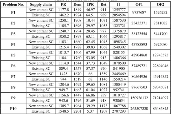
To solve the generated test problems, the competitive stage, as stated in section 3-1, is respected first. Based on this stage, selling prices, incentive buying prices, market share of supply chains and the amount of returned products, for each tactical period of the strategic periods is defined. The results of the competitive stage for all test problems are indicated in table 3. It should be noted that the average values of these variables with respect to all customer zones, tactical and strategic periods are reported in table 3.
Table 3. Competitive stage’s results
Problem No. Supply chain PR Dem IPR Ret OF1 OF2 P1 New entrant SC 1177.8 1849 46.97 911 1255777 9737687 1526232
Existing SC 1462.2 1924 64.51 989 2054594
P2 New entrant SC 1258.1 1908 10.44 1071 1587530 23433371 2811082 Existing SC 1105.7 1696 29.97 1053 1323721
P3 New entrant SC 1240.7 1794 28.45 977 1375879 38123554 5441700 Existing SC 1058.2 1897 63.11 1066 1295817
P4 New entrant SC 1103.1 1660 62.45 1045 1098345 43783893 6925080 Existing SC 1215.4 1788 39.83 1068 1549302
P5 New entrant SC 1013.7 1406 67.99 1044 820155 42904860 12743575 Existing SC 1104.1 1760 53.05 913 1486366
P6 New entrant SC 1114.9 1544 37.73 1049 1070500 57489721 22894046 Existing SC 889.4 1557 57.37 970 841900
P7 New entrant SC 1425 1670 66 1359 2445469 80564936 45914352
Existing SC 944 1519 68 1146 1550214
P8 New entrant SC 1204.6 1692 59.65 1081 1300449 87667503 59345081 Existing SC 949.7 1663 61.04 1027 952741
P9 New entrant SC 1156.6 1447 66.86 839 1010727 150926132 71214097 Existing SC 943.6 1596 51.69 918 938654
P10 New entrant SC 1385.7 1964 39.29 1173 1867788 265507330 86486845 Existing SC 1548.5 2201 5.37 1207 2707293
According to the calculated selling and buying prices and respecting the market share of supply chain in each customer zone, the new dynamic and integrated network design stage for the new entrant CLSC can be solved, as discussed in section 3.2.
Using MOICA to solve the network design stage leads a Pareto-front for each test problem. Two last columns of table 3 indicate the objective functions for each test problem. Since Pareto-front of each test problem includes several solutions, the average values for the objective functions are reported in table 3.
160
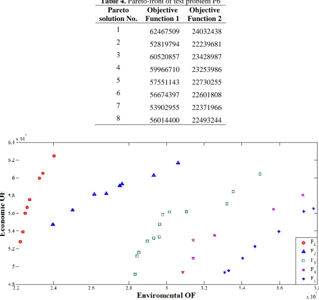
Furthermore, the objective functions of the final Pareto-front for test problem P6 are indicated in table 4. It is observed that using MOICA leads to 8 solutions which cannot dominate each other, so that the decision maker can select the desirable solution among them.
Figure 5 indicates the five last Pareto-fronts which are obtained from solving test problem P6 by MOICA. Accordingly, the improvement of solutions during sequential iterations can be observed in figure 5.
Table 4. Pareto-front of test problem P6
Pareto solution No.
Objective Function 1
Objective Function 2
1 62467509 24032438
2 52819794 22239681
3 60520857 23428987
4 59966710 23253986
5 57551143 22730255
6 56674397 22601808
7 53902955 22371966
8 56014400 22493244
161
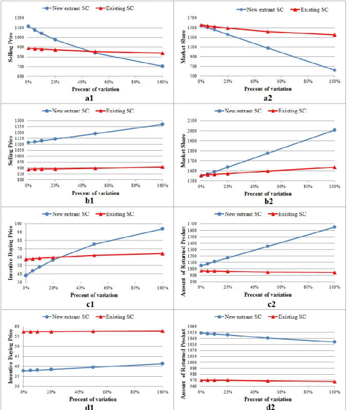
Fig 6. Sensitivity analysis of selling and buying prices’ eclasticity coefficient
4-2- Sensitivity analysis
Based on the interactions exist among the short-term pricing decisions and the strategic network design problem, in this section a sensitivity analysis on elasticity coefficients, is implemented for test problem P6.
162
Figure 6(a) indicates the impact of self-selling price elasticity coefficients (r k p, , ) on the market shares
( ,
,
n t k p
Dem ) and selling prices ( ,
,
n t k p
PR ).As it is expected, the market share and selling prices decrease when
, ,
r k p
increases. In fact, larger values for self-price elasticity coefficient (r k p, , ) result in more sensitivity of
market share to selling price of the relevant supply chain. So, the supply chain has to set smaller selling prices to attract more customers.
Figure 6(b) indicates the effect of cross-selling price elasticity coefficients (r k p, , ) on selling price
( ,,
n t k p
PR ) and market share ( ,
,
n t k p
Dem ). It is observed that r k p, , has a positive influence on the selling prices
and market shares which means increasing r k p, , encourages supply chain r to set higher selling prices,
so that its market share is increased, significantly.
Figure 6(c) indicates the changes of incentive buying price ( ,,
n t k p
IPR ) and the amount of returned product
( ,
,
Re n t k p
t ) with respect to the changes of self-buying price elasticity coefficients (r k p, , ). It is observed that
, ,
r k p
has influences on the buying price and the amount of returned products, positively.
Figure 6(d) confirms the negative impact of the cross-buying price elasticity coefficients (r k p, , ) on the
amount of returned products. As a result, the supply chain r has to increase the incentive buying prices to
compensate this disability.
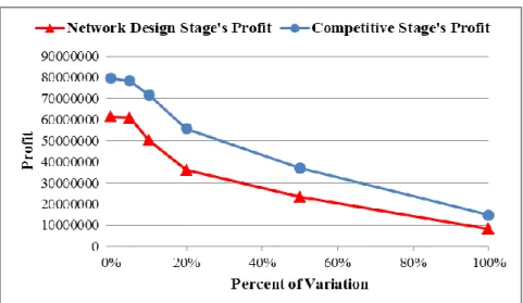
Finally, figure 7 indicates the effect of selling price’s elasticity coefficients on the economic objective functions for both competitive and network design stages. It is obvious that, increasing this parameter leads to less selling price and market share. Hence, the profit of supply chain is decreased. Since the fixed opening cost is not considered in the competitive stage, there is a difference between two stages’ profit. Also, the competitive stage is solved based on selling products in all customer zones, while some customer zones might be missed in the network design stage.
Fig 7. Variations of economic OF vs. selling price’s eclasticity coefficient
5- Conclusion
In this paper, a bi-objective model was proposed for the dynamic and integrated closed-loop supply chain network design problem in a competitive environment which attempted to optimize both economic and environmental concerns. The proposed dynamic model included several strategic periods. Furthermore, to integrate short-term tactical and operational decisions with strategic ones, multiple tactical periods were considered in each strategic period. Also, a chain to chain competition on selling prices of forward logistics and buying prices of reverse logistics was regarded. To solve the proposed
163
model, the competitive stage is considered first, in which the game theory approach is used to determine the optimal selling and buying prices. Based on these resulted prices in the model, the achieved bi-objective network design stage was solved using the Pareto-based multi-bi-objective imperialist competitive algorithm. Finally, the proposed model and solution approach were evaluated using several numerical examples.
In this paper selling and buying prices are considered as competitive factors, while the other competitive factors such as quality and service level can be regarded in the chain to chain competition. The model can also be extended by consideration of the uncertainty and different scenarios for the parameters. Finally, using bi-level programming approach in solving the proposed model may lead to more accurate and reliable results.
References
Accorsi, R. Manzini, R., Pini, C. & Penazzi, S. (2015). On the design of closed-loop networks for product
life cycle management: Economic, environmental and geography considerations”, Journal of Transport
Geography, 48, 121–134.
Atashpaz-Gargari, E., & Lucas, C. (2007). Imperialist Competitive Algorithm: An algorithm for optimization inspired by imperialist competition”, IEEE Congress on Evolutionary Computation.
Badri, H., Bashiri, M., & Hejazi, T.H. (2013). Integrated strategic and tactical planning in a supply chain
network design with a heuristic solution method. Computers & Operations Research, 40 (4), 1143–1154.
Bilir, C., Onsel Ekici, S., Ulengin, F. (2017). An integrated multi-objective supply chain network and
competitive facility location model. Computers & Industrial Engineering, 108, 136–148.
Deb, K., Pratap, A., Agarwal, S., & Meyarivan, T. (2002). A fast and elitist multi-objective genetic
algorithm: NSGA-II. IEEE Transactions on Evolutionary Computation, 6, 182–197.
Dubey, R., Gunasekaran, A., &Childe S.J. (2015). The design of a responsive sustainable supply chain
network under uncertainty. International Journal of Advanced Manufacturing Technology, 80 (1),
427-445.
Enayatifar, R., Yousefi, M., Abdullah, A.H., & Darus, A.N. (2013). MOICA: A novel multi-objective
approach based on imperialist competitive algorithm. Applied Mathematics and Computation, 219, 8829–
8841.
Fahimi, K., Seyedhosseini, S.M., & Makui, A. (2017a). A decentralized multi-level leader-follower game
for network design of a competitive supply chain, Journal of Industrial and Systems Engineering, 10(4),
1-27.
Fahimi, K., Seyedhosseini, S.M., & Makui, A. (2017b). Simultaneous competitive supply chain network
design with continuous attractiveness variables. Computers & Industrial Engineering, 107, 235–250.
Fallah, H., Eskandari, H., & Pishvaee M.S. (2015). Competitive closed-loop supply chain network design
under uncertainty. Journal of Manufacturing Systems, 37 (3), 649–661.
Fattahi, M., Mahootchi, M., Govindan, K., & Moattar Husseini, S.M. (2015). Dynamic supply chain
network design with capacity planning and multi-period pricing. Transportation Research Part E, 81,
169–202.
Fattahi, P., Hajipour, V., & Nobari, A. (2015). A Bi-objective Continuous Review Inventory Control
164
Ghavamifar, A, Sabouhi, F., & Makui, A., (2018). An integrated model for designing a distribution
network of products under facility and transportation link disruptions, Journal of Industrial and Systems
Engineering, 11(1), 113-126.
Govindan, K., Jafarian, A., & Nourbakhsh, V. (2015). Bi-objective integrating sustainable order allocation and sustainable supply chain network strategic design with stochastic demand using a novel
robust hybrid multi-objective metaheuristic. Computers & Operations Research, 62, 112-130.
Govindan, K., Soleimani, H., & Kannan, D. (2015). Reverse logistics and closed-loop supply chain: A
comprehensive review to explore the future. European Journal of Operational Research, 240, 603–626.
Hafezalkotob, A., Babaei, M.S., Rasulibaghban, A., & Noori-daryan M. (2014). Distribution Design of Two Rival Decenteralized Supply Chains: a Two-person Nonzero Sum Game Theory Approach.
International Journal of Engineering Transaction B: Application, 27, No. 8, 1233-1242.
Hosseini-Motlagh, S.M., Nematollahi, M., & Nouri, M., (2018). Coordination of green quality and green
warranty decisions in a two-echelon competitive supply chain with substitutable products, Journal of
Cleaner, 196, 961-984.
Kamali, H., Sadegheih, A., Vahdat-Zad, M. & Khademi-Zare, H. (2014). Deterministic and metaheuristic
solutions for closed-loop supply chains with continuous price decrease. International Journal of
Engineering, 27 (12), 1897-1906.
Kaya, O., Urek, B. (2015). A Mixed Integer Nonlinear Programming Model and Heuristic Solutions for
Location, Inventory and Pricing Decisions in a Closed Loop Supply Chain. Computers & Operations
Research, 65, 93-103.
Keyvanshokooh, E., Fattahi, M., Seyed-Hosseini, S.M., & Tavakkoli-Moghaddam R. (2013). A dynamic
pricing approach for returned products in integrated forward/reverse logistics network design. Applied
Mathematical Modelling, 37, 10182–10202.
Laari, S., Toyli, J., & Ojala, L., (2017). Supply chain perspective on competitive strategies and
green supply chain management strategies, Journal of Cleaner Production, 141, 1303-1315.
Liu, Z., Qiu, T., & Chen, B. (2014). A study of the LCA based biofuel supply chain multi-objective
optimization model with multi-conversion paths in China. Applied Energy, 126, 221-234.
Ma, P., Zhang, C., Hong, X., & Xu, H., (2018). Pricing decisions for substitutable products with green
manufacturing in a competitive supply chain, Journal of Cleaner Production, 183, 618-640.
Makui, A., & Ghavamifar, A., (2016). Benders Decomposition Algorithm for Competitive Supply Chain
Network Design under Risk of Disruption and Uncertainty, Journal of Industrial and Systems
Engineering, 9, 30-50.
MATLAB Version 7.10.0.499 (R2010a). The MathWorks, Inc. Protected by U.S. and international patents.
Melo, M.T., Nickel, S., & Saldanha-da-Gama F. (2009). Facility location and supply chain management –
165
Mota, B., Gomes, M.I., Carvalho, A., & Barbosa-Povoa A.P. (2014). Towards supply chain sustainability:
economic, environmental and social design and Planning. Journal of Cleaner Production, 105, 14-27.
Nagurney, A., Dong, J., & Zhang D. (2002). A supply chain network equilibrium model. Transport
Research Part E, 38, 281–303.
Nobari, A., Kheirkhah, A.M., & Esmaeili, M. (2016). Considering pricing problem in a dynamic and
integrated design of sustainable closed-loop supply chain network. International Journal of Industrial
Engineering and Production Research, 24 (4), 353-371.
Nobari, A., Kheirkhah, A.S., & Esmaeili, M, (2018). Considering chain-to-chain competition on
environmental and social concerns in a supply chain network design problem, International Journal of
Management Science and Engineering Management, https://doi.org/10.1080/17509653.2018.1474142.
Pishvaee, M.S., & Razmi, J. (2012). Environmental supply chain network design using multi-objective
fuzzy mathematical programming. Applied Mathematical Modelling, 36, 3433–3446.
Rahmani, D., & Mahoodian, V. (2017). Strategic and operational supply chain network design to reduce
carbon emission considering reliability and robustness. Journal of Cleaner Production, 149, 607–620.
Rabbani, M., Keshvarparast, A., & Farrokhi-Asl, H., (2016). Comparing supply side and demand side options for electrifying a local area using life cycle analysis of energy technologies and demand side
programs, Journal of Industrial and Systems Engineering, 9(4),1-8.
Rezapour, S., Zanjirani Farahani, R. (2010). Strategic design of competing centralized supplychain
networks for markets with deterministic demands. Advance in Engineering Software, 41, 810–22.
Rezapour, S., Zanjirani Farahani, R, Ghodsipour, S.H., & Abdollahzadeh, S. (2011). Strategic design of
competing supply chain networks with foresight. Advance in Engineering Software, 42, 130–41.
Rezapour, S., Zanjirani Farahani, R., & Drezner, T. (2011). Strategic design of competing supply chain
networks for inelastic demand. Journal of Operation Research Society, 62, 1784–95.
Saghaeeian, A., & Ramezanian, R., (2018). An efficient hybrid genetic algorithm for multi-product
competitive supply chain network design with price-dependent demand, Applied Soft Computing, 71,
872-893.
Shen, Z.J. (2007). Integrated supply chain design models: a survey and future research directions.
Journal of Industrial and Management Optimization, 3No. 1, 1–27.
Shi, J., Zhang, G., & Sha, J. (2011a). Optimal production and pricing policy for a closed loop system.
Resources, Conservation and Recycling, 55, 639–647.
Shi, J., Zhang, G., & Sha, J. (2011b). Optimal production planning for a multi-product closed loop system
with uncertain demand and return. Computers & Operation Researches, 38 (3), 641-650.
Simchi-Levi, D., Kaminsky, P., & Simchi-Levi, E. (1999). Designing and managing the supply chain: concepts, strategies, and cases. New York: McGraw-Hill.
Soleimani, H., Govindan K., Saghafi, H., & Jafari, H. (2017). Fuzzy multi-objective sustainable and green
166
Wu, X., Zhou, Y., (2017). The optimal reverse channel choice under supply chain competition, European
Journal of Operational Research, 259(1), 63-66.
Yazdi, A., Honarvar M. (2015). A Two Stage Stochastic Programming Model of the Price Decision
Problem in the Dual-channel Closed-loop Supply Chain. International Journal of Engineering
Transaction B: Application, 28 (5), 738-745.
Yousefi Yegane, B., Nakhai Kamalabadi, I., & Farughi, H. (2016). A Non-linear Integer Bi-level
Programming Model for Competitive Facility Location of Distribution Centers. International Journal of
Engineering Transaction B: Application, 29 (8), 1131-1140.
Zanjirani Farahani, R. Rezapour, S. Drezner, T. & Fallah, S. (2014). Competitive supply chain network