Robust sparse representation based multi focus image fusion with dictionary construction and local spatial consistency

Accepted Manuscript

Robust sparse representation based multi-focus image fusion with

dictionary construction and local spatial consistency

Qiang Zhang , Tao Shi , Fan Wang , Rick S. Blum , Jungong Han

PII:

S0031-3203(18)30213-9

DOI:

10.1016/j.patcog.2018.06.003

Reference:

PR 6577

To appear in:

Pattern Recognition

Received date:

31 October 2017

Revised date:

8 May 2018

Accepted date:

1 June 2018

Please cite this article as: Qiang Zhang , Tao Shi , Fan Wang , Rick S. Blum , Jungong Han , Robust

sparse representation based multi-focus image fusion with dictionary construction and local spatial

consistency,

Pattern Recognition

(2018), doi:

10.1016/j.patcog.2018.06.003

ACCEPTED MANUSCRIPT

Highlight

 A RSR model is introduced for multi-focus image fusion.

ACCEPTED MANUSCRIPT

Robust sparse representation based multi-focus image fusion

with dictionary construction and local spatial consistency

Qiang Zhanga,b, Tao Shib, Fan Wangb, Rick S. Blumc, Jungong Hand

a_{Key Laboratory of Electronic Equipment Structure Design, Ministry of Education, Xidian University, Xi'an, Shaanxi 710071,}

China

b

Center for Complex Systems, School of Mechano-electronic Engineering, Xidian University, Xi'an Shaanxi 710071,China

c_{Electrical and Computer Engineering Department, Lehigh University, Bethlehem, PA 18015, United States}

d_{School of Comping and Communications, Lancaster University, Lancaster, LA1 4YW, U.K.}

Abstract: Recently, sparse representation-based (SR) methods have been presented for the fusion of multi-focus images.

However, most of them independently consider the local information from each image patch during sparse coding and fusion, giving rise to the spatial artifacts on the fused image. In order to overcome this issue, we present a novel multi-focus image fusion method by jointly considering information from each local image patch as well as its spatial contextual information during the sparse coding and fusion in this paper. Specifically, we employ a robust sparse representation (LR_RSR, for short) model with a Laplacian regularization term on the sparse error matrix in the sparse coding phase, ensuring the local consistency among the spatially-adjacent image patches. In the subsequent fusion process, we define a focus measure to determine the focused and de-focused regions in the multi-focus images by collaboratively employing information from each local image patch as well as those from its 8-connected spatial neighbors. As a result of that, the proposed method is likely to introduce fewer spatial artifacts to the fused image. Moreover, an over-complete dictionary with small atoms that maintains good representation capability, rather than using the input data themselves, is constructed for the LR_RSR model during sparse coding. By doing that, the computational complexity of the proposed fusion method is greatly reduced, while the fusion performance is not degraded and can be even slightly improved. Experimental results demonstrate the validity of the proposed method, and more importantly, it turns out that our LR-RSR algorithm is more computationally efficient than most of the traditional SR-based fusion methods.

Key words: multi-focus image fusion, robust sparse representation, dictionary construction, spatial contextual information, spatial consistency.

1. Introduction

Due to the limited depth of field of optical lenses in conventional cameras, it is not often possible

to obtain an image that contains all of the relevant objects in focus [1, 2]. As shown in Fig. 1, this issue

can be effectively addressed by multi-focus image fusion, in which several images with different focus

points (e.g., Fig. 1 (a) and Fig. 1(b)) are combined into a composite image (e.g., Fig. 1(c)) with

full-focus.

Suppose at least one of the input images provides a focused version of the scene, the focused

regions can be extracted from the given multi-focus input images and then preserved in the fused image,

while all of the defocused regions should be discarded [1]. In addition, the fusion algorithm should not

introduce any spatial artifacts or inconsistencies into the fused image. Finally, the fusion algorithm

ACCEPTED MANUSCRIPT

should have high computational efficiency, thereby facilitating real-world applications. In this paper,

we will address the fusion of multi-focus images by using a robust sparse representation (RSR) model

with dictionary construction and local spatial consistency, specifically designed to have high spatial

consistency and computational efficiency.

Fig. 1. Illustration of multi-focus image fusion. (a) Source image with focus on the flower; (b) Source image with focus on the

clock; (c) Fused image with full-focus.

So far, many sparse representation-based (SR) methods have been presented for the fusion of

multi-focus images [1, 2, 3, 4, 5, 6, 7, 8, 9]. A thorough review of these methods can be found in [10].

Rather than being fixed in advance as those in the traditional multi-scale transforms (MSTs), most of

the over-complete dictionaries in SR are learned from a set of training images using some learning

methods, such as K-SVD [11]. Compared with the fixed basis functions, these over-complete

dictionaries contain richer basis atoms and are able to achieve more meaningful and stable

representations of the source images. For this reason, SR-based image fusion methods generally

outperform the traditional MST-based image fusion methods from both subjective and objective aspects

[3, 4].

However, most of the existing SR-based fusion methods advocate the patch-based implementation.

More specifically, each image patch is individually taken into account during sparse coding and fusion,

giving rise to the spatial artifacts on the fused image. In order to reduce the spatial artifacts, a sliding

window technology [3] is often employed in these methods, where the input images are divided into a

larger number of patches overlapped with a fixed number of pixels (usually one pixel) along the

horizontal and vertical directions, respectively. Owing to the overlap among image patches, the number

of input patches to be fused is greatly large, which results in a huge requirement of memory storage and

increase of computational complexity. In addition, some detailed information will be unavoidably lost

in the fused image because of the overlap [1, 5].

In fact, images have strong local correlations among spatially adjacent patches. More precisely,

ACCEPTED MANUSCRIPT

these patches are either all in-focus or are all out-focus in most cases. Motivated by the observation, the

contextual information among spatially adjacent patches, instead of the sliding window approach, is

employed to reduce the spatial artifacts of the fused image in this paper. In addition, we pay special

attention to reducing the computational complexity of the proposed method in order to improve its

utility for real world applications.

To this end, we employ a robust sparse representation (LR_RSR, for short) model with a

Laplacian regularization term on the sparse error matrix during the sparse coding phase, which

adequately considers the local consistency among the spatially-adjacent image patches. In the

subsequent fusion process, we collaboratively employ information from each local image patch as well

as those from its spatial neighbors to determine the focused and de-focused regions in the multi-focus

images. By doing that, the spatial artifacts in the fused image may be obviously suppressed. Moreover,

owing to the joint use of sparse errors from multiple spatially adjacent patches, a non-overlapping

division of input images, rather than an overlapping division way as in most of SR-based fusion

methods, may be adopted during the fusion process. This greatly reduces the requirement of memory

storage and computational complexity of the proposed fusion method.

In addition, we will employ a learned dictionary with only a fixed small number of atoms but

maintaining good representation capability, rather than the input data themselves as in [1], for the

LR_RSR model during sparse coding. This will further greatly reduce the computational complexity of

the proposed method, while the fusion performance is not degraded and even slightly improved.

Experimental results demonstrate that the proposed method introduces fewer spatial artifacts to the

fused images than most state-of-the-art methods. Especially, it is also shown to have higher

computational efficiency than some traditional SR-based fusion methods.

In summary, the main contributions of this paper are as follows.

(1) We present a multi-focus image fusion algorithm based on a robust sparse representation (RSR)

model, in which the spatial consistency among image patches is adequately considered during

sparse coding and fusion. This is clearly different from most of the existing SR-based fusion

methods, which usually treat each image patch independently.

(2) We employ a robust sparse representation (LR_RSR) model with a Laplacian regularization on the

sparse error matrix during sparse coding. To the best of our knowledge, it is the first time that the

ACCEPTED MANUSCRIPT

over-complete dictionary with small atoms while maintaining good representation capability for

the LR_RSR model.

(3) We jointly employ local information (i.e., sparse reconstruction errors obtained by LR_RSR) of

each image patch along with those from its spatially adjacent neighbors to determine the focused

and defocused regions within an input multi-focus image during the fusion process.

The rest of the paper is organized as follows. Section 2 briefly reviews the SR-based fusion

methods. Section 3 details the dictionary construction for RSR model. Section 4 describes the proposed

fusion method in detail. Experimental results and conclusions are given in Section 5 and Section 6,

respectively.

Notations

Throughout the paper, a vector is denoted by a lower-case letter, and a matrix is denoted by a

capital letter. All elements of vectors and matrices are real-valued. Given a vector x and a matrix X,

some notations used in this paper are listed in Table 1.

Table 1. List of vector and matrix related notations.

Symbols Definition

( )

x i _{the i-th entry of the vector x}

( , )

X i j _the

 

_{i j, -th entry of the matrix X}

( ,:)

X i _{the i-th row of the matrix X}

(:, )

X j _{the j-th column of the matrix X}

2

x _l

2-norm of the vector x, i.e., x₂



_ix i2( )

0,2

X l0,2-norm of the matrix X, i.e., the number of the non-zero rows in the matrix X

1,2

X _{l1,2-norm of the matrix X, i.e.,} 2 1,2 i j ( , )

X 

 

X i j

2,0

X l2,0-norm of the matrix X, i.e., the number of the non-zero columns in the matrix X

2,1

X _l

2,1-norm of the matrix X, i.e., X_2,1

 

_{j i}X i j2( , ) F

X _{Frobenius-norm of the matrix X, i.e.,} 2 , ( , )

F i j

X 



X i j

X _ l-norm of the matrix X, i.e., the maximum absolute value of the entries in the matrix X

 

T

 transpose of a vector or a matrix

2. Related work

To date, numerous fusion algorithms have been presented for multi-focus images [12, 13, 14],

wherein multi-scale transform-based (MST-based) image fusion algorithms are one of the most popular

choices [15]. Various MST-based fusion methods have been discussed over the years, ranging from the

early wavelet [16] and pyramid [17] transforms to the recently developed multi-scale geometric

analysis approaches, such as curvelet [18], contourlet [19], and shearlet [20].

ACCEPTED MANUSCRIPT

representation (SR) has also attracted more attention in multi-sensor image fusion, including

multi-focus image fusion, in recent years [1-9, 21-24]. For example, in [3], Yang and Li first introduced

SR [25] into image fusion, where the l₁-norm of the SR coefficient vector (i.e., the sum of the absolute

values of SR coefficients) was employed as the activity level for each local image patch and the fused

image was constructed using a maximum selection fusion rule. A SR model with dictionary learning

was presented for multi-focus image fusion in [2], where the correlation between the sparse

representation coefficients of input image patch and the pooled features obtained in the dictionary

learning phase, instead of the simple l₁- orl₂-norm of the representation coefficient vector, was used

as the activity level. In [4], a general image fusion framework was presented by combing MST and SR

to simultaneously overcome the drawbacks of the MSR-based and SR-based fusion methods. They also

presented an adaptive SR (ASR) model for simultaneous image fusion and denoising [21]. In [6], a

group sparse presentation (GSR) model was presented to exploit the intrinsic structure among the

atoms in different groups and applied to medical image fusion, where the non-zeros elements are forced

to occur in clusters (i.e., group-sparsity) rather than appear randomly. Almost all these SR-based fusion

methods are performed in a patch-based way. Alternatively, a newly merged convolutional SR (CSR)

model was introduced to image fusion [5], which aims to achieve the SR of an entire image rather than

a local image patch.

In [1], a robust SR (RSR) model was first presented to extract the detailed information in a set of

multi-focus images by using a so-called sparse reconstruction error, instead of the conventional

least-squared reconstruction error. Then a multi-task RSR (MRSR) model was presented for

multi-focus image fusion by imposing a joint constraint on the reconstruction errors across all tasks. In

the MRSR-based fusion method, information from each local image patch and those from its spatial

neighbors (referred to as its spatial contextual information) were collaboratively employed to

determine the focused and de-focused regions. Owing to the use of spatial context, block artifacts in the

fusion results are greatly reduced and sometimes can even be eliminated.

Despite its great advances in terms of the performance, MRSR is computationally expensive,

especially when the number of spatially adjacent patches of each image patch gets increased. In

addition, the data is directly employed as the dictionary in the MRSR model. With an incremental size

of each input image, the computational complexity of MRSR increases again, eventually leading the

ACCEPTED MANUSCRIPT

Similar to that in [1], we also consider the spatial context among image patches during the fusion

process in this paper. But differently, we pay special attention to reducing the computational

complexity of the proposed fusion method.

3. Dictionary construction for RSR model

Owing to the obvious superiority of RSR over the traditional SR [25], we also employ the RSR

model [1] to achieve the sparse coding of each image patch. In addition to the RSR model, the

employed over-complete dictionary also plays an important role for the fusion performance and

computation efficiency of a multi-focus fusion method. In [1], the data themselves were simply

employed as the dictionary during the sparse coding. Despite its excellent performance, the downside

of such an approach is that the computational burden can be excessive for larger images if the number

of dictionary atoms is propositional to the image size.

Alternatively, we will present a simple but efficient dictionary construction method for RSR. For

that, we will first construct a set of data samples (or image patches), denoted by a matrix

1 2

[ , ,..., N] n N

Y  y y y R of size n N , which are randomly selected from a set of training images.

Here, n denotes the dimension of each data sample and N denotes the total number of image

patches. Each column y_iRn of the matrix Y represents a data vector (i.e., a training image patch).

Then we will find an optimal subset of the data samples set Y , rather than the whole set Y , to form

the dictionary

1 2

[ , ,..., ]

M

n M i i i

D y y y R where i i1, ,...,2 iM 



1, 2,...,N



, such that any column from

Y can be well reconstructed by the subset D.

We will achieve this goal by first formulating the problem as the following robust "row-sparsity"

optimization problem, similar to that in [26].

0,2 2,0

,

min . .

X E X  E s t YYXE. (1)

Here, [ ,_{1 2},..., ] N N N

X  x x x R  is the representation coefficient matrix to be sought, and each of its

columns x_iRN denotes the representation coefficients for the data y_i. Note that YX denotes the

authentic information contained in the data samples Y.

E



R

n N is the sparse error matrix and

denotes the corruptions or outliers within the data samples Y. The parameter 0 _{is to balance the}

effects of the two components in (1) and is experimentally set to 30 in this paper.

ACCEPTED MANUSCRIPT

dictionary in (1). However, the goal of [27] is to achieve the sparse coding for the input data using a l0 -

or l1 -norm minimization constraint, while our goal is to construct a dictionary for the RSR model by

selecting only a small number of image patches with sufficient representation capability from the input

training patches. Therefore, a "row-sparsity" (i.e., l0,2-norm minimization) constraint is employed in

(1).

When solving (1), the optimal solution of the representation coefficient matrix

X

* may be

incentivized to have some “zeros” rows because of the “row-sparsity” (i.e., l0,2-norm minimization)

constraint, which means that the corresponding data samples in the matrix Y are not used to reconstruct

any data samples during the coding and thus cannot be selected as the dictionary atoms. In contrast, the

data samples corresponding to the “non-zeros” rows in the matrix *

X

have been used to reconstruct

the other data samples. In fact, those data samples corresponding to the rows with larger energies (i.e.,

those row vectors with larger l2-norm values) get higher weights during the coding phase, and can thus

be deemed to be more important. Therefore, we will select those data samples corresponding to the row

vectors of the optimal matrix

X

* with the M largest l2-norm values as the dictionary atoms, i.e.,

1 2

[ , ,..., ]

M

i i i

D y y y with * * * *

1 2 1 2

2 2 2 2

(:, ) (:, ) (:,M) (:, ) , , ,...,M

X i  X i   X i  X j ji i i . Here, we

experimentally set M to 128 or 256, which is far smaller than the total number of data samples N.

Next, we discuss the details of solving (1), which is a non-convex optimization problem and can

be relaxed to the following convex one

1,2 2,1

,

min . .

X E X  E s t YYXE. (2)

The optimization problem in (2) is convex and can be solved by various methods. Here, we adopt the

linearized alternating direction method with an adaptive penalty (LADMAP) [28, 29] considering that

LADMAP has high computational efficiency and a convergence guarantee for such convex

optimization problems as in (2). In addition, LADMAP can also ensure each sub-problem mentioned in

(2) to have a closed-form solution. In LADMAP, an augmented Lagrangian function is first constructed

by introducing a Lagrange multiplier to remove the equality constraint as

2

1,2 2,1

,

2

1,2 2,1

,

min + , +

2

min +

2

F X E

X E

F

J X E V Y YX E Y YX E

V

X E Y YX E

 

 



     

    

, (3)

ACCEPTED MANUSCRIPT

product of the matrices A and B. Then the objective function in (3) is alternately minimized with

respect to X and E, respectively, by fixing one or the other. Algorithm 1 gives the optimization

algorithm for dictionary construction.

Algorithm 1: Optimization of RSR with “row-sparsity” constraint

Input: Sampling data Y and parameter 

Output: Representation coefficient and error matrices X and E

Initialize1_: 0

X 0, 0

E 0,1.1,106, 10

max 10

  , 4

10 _ 

while not converged do

(1) Fix X and update E:

2 2 1 2,1 2,1 1 min min 2 2

j j j

j j j

j j j

E E

F F

V V

E  E  Y YX E  E Y YX E

  

 _{          . (4)}

This sub-optimization problem has the following closed-form solution [30]:



2



1 2

2

(:, ) /

(:, ), if (:, ) / (:, ) (:, ) 0, otherwise j j j G i

G i G i

E i G i

            

, (5)

where

j j

j V G Y YX _ . (2) Fix E and update X:

2

1 1

1,2 1,2

min min ( )

2

j j

j j j

j

X X

F

V

X X  Y YX E X f X



 _{   }  _{  }

, (6)

where 2 1 ( ) 2 j j j j j F V

f X  Y YX E

 

    . To solve (6), the quadratic termf X( )can be replaced by its first order

approximation at the previous iteration by adding a proximal term [31], i.e.,

 

 

2

2 1

1,2 1,2

min , min

2 2

j

j j

X

j j j j j

X j

F

X X

F f X

X X  X X f X X X X  X X



 _{         } _{, (7)}

where  is set to Y 2₂ as in [31].

 

j Xf X

 is the partial differential of f X

 

with respect to X, and is

computed by

 

1

j

j j T j j

X j

V

f X Y YX Y E

 

 

  _    _

 . Then (6) has the following close-form solution [30]:

2 1 2 2 1 ( ,:) 1 ( ,:), if ( ,:)) ( ,:) ( ,:) 0, otherwise j j j H i

H i H i X i H i     _      _    

, (8)

where 1 1

j

j T j j

j

V

H X Y YX Y E

  

 

  _    _

 .

(3) Update the multiplier V: Vj1Vjj



YYXj1Ej1



(4) Update : 1 min



, max



j j

 _  

(5) Check the convergence conditions: 1 1 1 1

, ,

j j j j j j

F F

Y YX  E Y  X  X  E E 

 

      

end while

4. RSR-based multi-focus image fusion with local spatial consistency

In this section, we will first present a RSR model with Laplacian regularization (LR_RSR, for

short) considering the local spatial consistency among image patches and then discuss how we apply it

to the fusion of multi-focus images.

4.1 RSR with Laplacian regularization (LR_RSR)

ACCEPTED MANUSCRIPT

Given the over-complete dictionary

D



R

n M constructed in the previous section, the existing

RSR model in [1] can be computed by

0 2,0

,

min . .

X E X  E s t YDXE

, (9)

where [ ,_{1 2},..., ] n N N

Y  y y y R is the observed data matrix (e.g., a multi-focus image in this paper),

and each of its columns is a data vector (e.g., an image patch) y_iRn.

X



R

M N and

E

n N denote

the representation matrix and error matrix, respectively.

Fig. 2. Illustration of the decomposition of RSR on a multi-focus image (Credit to [1]). Y denotes an image focused on the flowerpot. DX denotes a fully defocused version of the original and E contains the details of the flowerpot.

The RSR model in (9) can be directly applied to the fusion of multi-focus images similar to many

of the traditional SR-based fusion methods. Especially, as shown in Fig. 2, a multi-focus image can be

decomposed into a blurred or fully-defocused entity plus a detailed entity, denoted by the reconstructed

matrix DX and the error matrix E, respectively, by using the RSR model. In other words, the error

matrix E, rather than the representation coefficients, contains the high frequency details in the

multi-focus image and can thus be used to determine the focus measure of each multi-focus input

image [1].

However, as shown in (9), the traditional RSR model considers each local image patch

independently with no consideration of the local spatial consistency among image patches. As a result

of that, some spatial artifacts will be easily introduced to the fused image in the subsequent fusion

processing. In fact, images have strong local correlations among spatially adjacent patches. More

exactly, for a multi-focus image, the spatially adjacent image patches have similar focus information,

i.e., these patches are all in-focus or are all out-focus in most cases. Accordingly, they will also have

similar sparse errors in the RSR model.

ACCEPTED MANUSCRIPT

short) by integrating a Laplacian regularization with respect to the sparse error matrix with the

traditional RSR model in this paper as

1 2

0 2,0

,

min + ( T) . .

X E X  E tr ELE s t YDXE

, (10)

where



1 and



2 are two positive trade-off parameters to balance the three components. The

Laplacian regularization term ( T)

tr ELE is defined by

2

2 ,

1

( ) (:, ) (:, )

2

T

ij i j

tr ELE 



E i E j  . (11)

The weight



_ij implies the similarity between the i-th and j-th image patch and is computed by

2

2 2

exp , if and are spatially adjacent 2

0, otherwise

i j

i j

ij

y y

y y

 

  _ 

 _ 

 _{ }

  _{ }

 

. (12)



is a scalar parameter and is experimentally set to 0.5 in this paper. Based on these weights, an

affinity matrix _W_RN N _{with ( , )} ij

W i j 



and a diagonal degree matrix N N with

( , ) ( , )

j

i i W i j

 



are constructed. Then the Laplacian matrix L in (11) is computed by

L

  

W

.

In general, the spatially adjacent patches with similar appearances will have similar representation

coefficients as well as sparse errors in the RSR model. Accordingly, it might be more reasonable to

introduce two Laplacian regularization terms with respect to the representation coefficient matrix and

the sparse error matrix in (10), respectively. However, in this paper, the focus information of each local

patch in a multi-focus image is determined by its sparse errors rather than its representation coefficients.

Therefore, in (10), only one Laplacian regularization term with respect to the sparse error matrix is

introduced for simplicity.

The Laplacian regularization with respect to sparse error matrix in the proposed LR-RSR model

ensures the local consistency among the spatially-adjacent image patches. More specifically, each

column y_i in the observed matrix Y in (10) denotes an image patch to be considered when LR-RSR

is applied to multi-focus image fusion in our revised manuscript. The corresponding column E(:, )i in

the error matrix E denotes the sparse error for the i-th image patch. As shown in (12), if two spatially

adjacent image patches y_i and y_j have similar appearances, the weight



_{i j,} will be assigned to a

high value. Then the difference between E(:, )i and E(:, )j will be forced to be a small value by

ACCEPTED MANUSCRIPT

two image patches will thus be seen as both in-focus or both out-focus. As a result of that, the spatial

artifacts introduced into the fused image will be reduced to some extent.

Algorithm 2: Optimization of LR_RSR using LADMAP

Input: Observed data Y, over-complete dictionary D, and parameters 1,2

Output: Representation coefficient and error matrices X and E

Initialize: 0

X 0, 0

E 0,1.1,106,max1010, 3 10 _ 

while not converged do

(1) Fix E and update X:

2 1

1 1

min min ( )

2 j j j j j X X F V

X X  Y DX E X g X



 _{      }

, (15)

where 2 ( ) 2 j j j j F V

g X  Y DX E



    . Similar to that in solving (6), this sup-optimization problem can be solved by

replacing the quadratic termg X( ) with its first order approximation at previous iteration and a proximal term, i.e.,

 

 

2

2

1 1 1

1 1

1

min , = min

2 2

j

j j

X

j j j j j

X j

F

X X

F g X

X  X   XX   g X XX X   XX _{ } , (16)

where 1 is set to 2

1 Y 2

  and Xg X

 

j is computed by

 

1

j

j j T j j

X j

V

g X  D DX Y E

 

 

  _    _

 . Thus it has the following closed-form solution [32]:

1 1 1 1 1 1 j j

j j T j j

j

V

X S X D DX Y E

   

 _ _{ }  _{ }  _ _

 

 _{ }

 , (17) where the threshold function S x( ) is defined as

, if ( ) , if

0, otherwise

x x

S x x x

             

. (18)

(2) Fix X and update E:

2

1 1

1 2,1 2 2,1

min ( ) min ( )

2

j j

j T j

j

E E

F

V

E  E tr ELE  Y DX E E h E



 _{   }  _{    , (19)}

where 2 1 2 ( ) ( ) 2 j j T j j F V

h E tr ELE  Y DX E

 

     . Similarly, this sub-optimization problem can be solved by

 

 

2 2

1 2 1

1 2,1 2,1

2 2

1

min , min

2 2

j E

j j j j j

E F

E E

F

h E

E  E  E E h E E E  E E E

 

 _{         } _{, (20)}

where 2 is set to





2 2 1.02 2 2

j F

L

    as suggested in [33]. Eh E

 

j is computed by

1 2

( ) 2

j

j j j j j

E j

V h E E L  Y DX  E _ 

       

 . Thus it has the following closed-form solution [30]:



2



1 2 1 2

2

(:, ) /

(:, ), if (:, ) / (:, ) (:, )

0, otherwise

j j

Q i

Q i Q i

E i Q i

            

, (21)

where

 

2

j E j h E

Q E

 

  .

(3) Update the multiplier V: Vj1Vjj



YDXj1Ej1



(4) Update : 1 min



, max



j j

 _  

(5) Check the convergence conditions: 1 1 1 1

, ,

j j j j j j

F F

Y DX  E Y  X  X  E E 

 

      

end while

Similar to the case in the previous section, the non-convex optimization problem in (10) can be

ACCEPTED MANUSCRIPT

1 2

1 2,1

,

min + ( T) . .

X E X  E tr ELE s t YDXE. (13).

Then an augmented Lagrangian function is constructed by introducing a Lagrange multiplier to remove

the equality constraint as

2

1 2

1 2,1

,

2

1 2

1 2,1

,

min + ( ) ,

2

min + ( )

2

T

F X E

T

X E

F

J X E tr ELE V Y DX E Y DX E

V

X E tr ELE Y DX E



 



 



       

     

. (14)

Finally, the optimization problem can be solved by using the LADMAP method [28, 29]. Algorithm 2

provides the optimization of LR_RSR in detail.

Fig. 3. Illustration of the validity of the Laplacian regularization term in the LR_RSR model. (a) An image with focus on the flower; (b) Sparse errors obtained using the traditional RSR model; (c) Sparse errors obtained using the LR-RSR model.

Fig.3 illustrates the validity of the Laplacian regularization term in the LR_RSR model. As shown

in Fig. 3(b), parts of the clock regions also have higher sparse errors by using the traditional RSR

model in addition to the flower regions. As a result of that, parts of the clock regions in Fig. 3(a) will be

mistakenly determined to be in-focus in the subsequent fusion process by using the RSR model, thus

introducing some spatial artifacts to the fused image. In contrast, as shown in Fig. 3(c), only the

focused flower regions are forced to have high sparse errors and will be determined to be in-focus by

using the LR-RSR model.

Furthermore, the introduction of the Laplacian regularization does not increase the computational

complexity of the LR_RSR model. Similar to the traditional RSR, the major computational complexity

ACCEPTED MANUSCRIPT

matrices. As a result, LR_RSR has the same computational complexity as RSR. MRSR may also

ensure the spatial consistency among image patches to some extent by imposing a joint sparsity

constraint (i.e. l2,1-norm minimization) on the reconstruction errors across all tasks. However, the joint

sparsity constraint increases the computational complexity of MRSR.

More specifically, suppose the data matrix Y and dictionary D have sizes of n N and

n M , respectively. Then the coefficient matrix X has size MN . Thus, the computational

complexities of RSR and LR_RSR are both O rnNM( 2) by further considering the number of

iterations r needed for convergence. While, the computational complexity of MRSR is about

2

( )

O rnKNM , where K denotes the number of spatially adjacent patches for each image patch to be

considered. Here, the number of dictionary atoms M_k for all types of features in the MRSR model are

assumed to be the same, i.e., M₀M₁ M_K1M. For this reason, we will apply LR_RSR to

multi-focus image fusion in the following subsection.

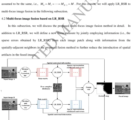
4.2 Multi-focus image fusion based on LR_RSR

In this subsection, we will discuss the proposed multi-focus image fusion method in detail. In

addition to LR_RSR, we will define a new focus measure by jointly employing information (i.e., the

sparse errors obtained by LR_RSR) from each image patch along with information from the

spatially-adjacent neighbors in the proposed fusion method to further reduce the introduction of spatial

artifacts in the fused image.

Fig. 4. Diagram of the proposed fusion method.

[image:15.595.73.498.322.711.2]

ACCEPTED MANUSCRIPT

registered, the diagram of the proposed multi-focus image fusion algorithm based on LR_RSR is

shown in Fig. 4 and described as follows.

(1) Divide the input images IA and IB into N non-overlapping image patches of the same

size p_xp_y pixels. Then two sets of image patches



IiA|i0,1,...,N1



and



IiB|i0,1,...,N1



are obtained from images IA and IB, respectively.

(2) Re-order each image patch as a vector of dimension d p_xp_y and construct the data

matrices ₀A, ₁A,..., A₁

A N

Y  y y y _ _ and ₀B, ₁B,..., B₁

B N

Y  y y y __ for images IA and IB , respectively.

A i

y and y_iB are vectors corresponding to the i-th image patches I_iA and I_iB of images I_A and

B

I , respectively.

(3) Perform LR_RSR on Y_A and Y_B, respectively, using Algorithm 2 and then obtain their

corresponding representation coefficient matrices X_A, X_B and error matrices E_A, E_B. In this step,

a globally-trained dictionary D is employed, which is constructed from a set of training image patches

by using Algorithm 1. As well, each image patch and one of its 8-connencted neighbors are seen as a

pair of spatially-adjacent image patches during the computation of Laplacian regularization in (10).

(4) Define a decision map (i.e., a matrix)

C

with the same size of source images by using the

sparse errors EA and EB. The values of the entries in the matrix

C

are in the range of [0,1] . “1”

indicates that the fused pixels are directly selected from the source image I_A, while “0” means that

the fused pixels are directly selected from the source image I_B. Otherwise, the fused pixels are the

weighted average of the source images I_A and I_B . This step is one of the most important

components in the proposed fusion method and will be further discussed soon in detail.

(5) Construct the finally fused image IF by using the decision map

C

as



,





,

 

,





,





1



,





F A B

I m n I m n C m n I m n C m n , (22)

where I_F



m n,



, I_A



m n,



and I_B



m n,



denote the pixel values of the fused image IF , input

ACCEPTED MANUSCRIPT

the ( , )m n -th entry of the matrix (or the decision map)

C

.

In the following content, we will discuss the determination of the decision map

C

in detail.

First, define an initial decision map

C



_{of the same size} IA or IB, and divide the decision

map

C



into N patches of size p_xp_y by using the same way as that in the division of source image

A

I or I_B. Then obtain a set of decision map patches or sub-matrices



C ii | 0,1,...,N1



.

Secondly, assign each of its entries C m n_i( , ) in the i-th decision map patch C_i to “1” or “0” by

comparing the focus measure value



_iA of image patch I_iA with the focus measure value



_iB of

image patch I_iB as

1, if ( , )

0, otherwise

A B

i i

i

C m n  







 . (23)

Here, the focus measure value



_iA is patch-based and is jointly determined by the sparse errors of

image patch I_iA as well as its 8-connencted spatial-adjacent neighbors, denoted by ( A)

i

I

 , as follows

 

2 2

(:, ) A A (:, )

j i

A

i EA i I I EA j

  



_ . (24)

Accordingly, the focus measure value



iB is determined by using the same way, i.e.,

 

2 2

(:, ) B B (:, )

j i

B

i EB i I I EB j

  



_ . (25)

It should be noted that the sparse errors of current image patch and its spatially-adjacent neighbors,

instead of the only sparse error of current image patch, are jointly employed to define the focus

measure in (24) and (25). This will reduce spatial artifacts, as shown in Fig. 5(e).

Thirdly, reconstruct the decision map

C



by adding the patches



C i_i | 0,1,...,N1



to

C



at

their original spatial positions in

C



. This can be seen as the reverse process of the division of

C



.

Fourthly, refine the decision map

C



by removing some "holes" with small areas to obtain a new

decision map

C



. Although the introduction of local consistency can reduce the artifacts to great

extent, some isolated regions in-focus are still inevitably mistaken as de-focused ones. Similarly, some

isolated regions out-focus are also mistakenly labeled as the focused ones. As a result of that, there will

ACCEPTED MANUSCRIPT

numbers of entries are less than 5% of the total number of pixels in the input image are seen as isolated

regions and are thus removed. This is simply achieved by re-assigning the entry values within these

isolated regions as 1 minus their original values. The new decision map

C



is thus computed by





1 ( , ), if



,



,

( , ), otherwise

C

C m n m n

C m n

C m n

       _{ } 

 , (26)

where _C denotes the isolated regions in the decision map

C



.

Finally, define some transitional regions between the focused regions and the defocused regions,

and then construct the final decision map

C

. According to the decision map

C



, each input image

can be simply divided into two types of regions, i.e., focused regions and de-focused regions. For

example, “1” means focused regions while “0” means de-focused regions for imageIA. In contrast, “1”

and “0” mean de-focused regions and focused regions, respectively, for imageIB. However, as

discussed in [34], the de-focused imaging system can be characterized by a low-pass filtering system.

This indicates that it is a gradual process, rather than an abrupt process, from the focused (or

de-focused) regions to the de-focused (or focused) regions. In other words, it is reasonable to define a

transitional region between a focused region and a defocused region.

Therefore, in this paper, we will divide each multi-focus input image into three types of regions

(i.e., focused, de-focused and transitional regions), instead of two types of regions. We simply take

those patches in the decision map

C



as transitional regions, denoted by C, whose entries values

are different from those of one of its 8-connected spatial neighbors. For these transitional regions, the

fused image is computed as the weighted average of source images, instead of being simply selected

from one of the source images. Here, the weights are also computed by using the focus measure values

of these source image patches. Then the final decision map

C

is determined by

















1, if & ,

, , ,

0, if & ,

A B

i i C

A i C A B i i A B

i i C

m n

C m n m n

m n                 _      _{  } 

, (27)

where the index i in _iA or _iB is determined by the index of image patch I_iA or I_iB that the

location ( , )m n belongs to. By using the final decision map

C

, the fused image can be obtained by

ACCEPTED MANUSCRIPT

Fig. 5. Illustration of decision maps obtained by different methods. (a) Source image with focus on the ‘clock’; (b) Source image

with focus on the ‘student’; (c) ‘Ideal’ decision map; (d) Decision map obtained by using the sparse error of each single image patch; (e) Decision map C obtained by using the joint sparse errors of each image patch and its neighbors, i.e., (23); (f) Decision map C obtained by performing ‘removing holes’ on (e), i.e., (26); (g) Final decision map C by using (27), in which the gray regions denote the transitional regions.

Fig. 5 illustrates the decision maps obtained by different methods. As shown in Fig. 5(d), there are

many isolated patches or “holes” in the decision map obtained by using the sparse error of each single

image patch. In contrast, as shown in Fig. 5(e), these “holes” are greatly reduced by using the joint

sparse errors of each image patch and its spatially-adjacent neighbors. This demonstrates the

effectiveness of the proposed focus measures defined by (24) and (25). By further removing the

remaining “holes” or isolated patches, the decision map can be closer to the ‘ideal’ decision map.

4.3 Computational Complexity of the proposed fusion method

The computational complexity of the proposed fusion method is fully dependent on that of the

LR_RSR model. As discussed in Subsection 4.1, the computational complexity of LR_RSR is

2

( )

O rnNM , where M and N denote the numbers of the dictionary atoms and input image patches,

respectively. n denotes the dimension of the dictionary atoms or input data. r is the number of iterations

needed for convergence. Accordingly, the computational complexity of the proposed fusion method is

also _{O rnNM(} 2_{), which demonstrates that the number of dictionary atoms M has a greater impact}

on the computational complexity of the proposed fusion method than other parameters.

When RSR and MRSR are applied to multi-focus image fusion, the input data themselves are

simply employed as the dictionary in [1]. That is to say, the number of dictionary atoms M equals that

of the data (or the input image patches) N in the RSR-based and MRSR-based fusion methods. As a

ACCEPTED MANUSCRIPT

about O rnN( 3) and O rnKN( 3), respectively. Here K denotes the number of spatially adjacent

patches for each image patch to be considered. In addition, the number of dictionary atoms M (e.g.,

256 in this paper) is usually smaller than the number of image patches N (e.g., 1200 for an image of

size 320 240 ) in the proposed fusion method. Therefore, the proposed fusion method has greatly

higher computation efficiency than the RSR-based and MRSR-based fusion method.

More importantly, due to the non-overlapping division of input images, the number of image

patches N in the proposed fusion method is also much smaller than those (e.g., about 76800 for an

image of size 320 240 ) in the traditional SR-based fusion methods, including the RSR-based one in

[1], where an overlapping division way is usually adopted. Therefore, the proposed fusion method also

has higher computational efficiency than those traditional SR-based fusion methods. This will be

verified in the experimental part.

5. Experimental results and analysis

In this section, several sets of experiments are performed to verify the feasibility of the proposed

multi-focus image fusion algorithm based on the LR_RSR. First, we discuss the validity of the

constructed dictionary by using Algorithm 1. Then we discuss the impacts of some parameters on the

fusion performance. Finally, several pairs of multi-focus images from two public databases are fused

by using the proposed method and some state-of-the-art methods to demonstrate the validity of the

proposed method.

5.1 Validity of the constructed dictionary

Here, we will discuss the impacts of different dictionaries on the fusion performance to show the

validity of the proposed dictionary construction method. For that, 20,000 patches of size 8 8 are

first randomly selected from a set of images with high resolution to construct the training data. These

images are downloaded from http://r0k.us/graphics/kodak. Afterward, two sets of dictionaries with

different parameters are constructed by using Algorithm 1. One set of dictionaries (D_1,D_10,D_20,

30

D_ ,D_40,D_50,D_70and D_100, for short, respectively) are constructed by using the same

number of atoms (i.e., M=256) but different values of the parameter  _(i.e., =1, 10, 20, 30, 40, 50, 70, 100, respectively). The other set of dictionaries (D_M128,D_M256, D_M512, D_M1024 and D_M2048,

ACCEPTED MANUSCRIPT

the previous Fig. 5(a) and Fig. 5(b) are fused using the proposed fusion method but with different

dictionaries constructed above. In addition, the dictionary with 256 atoms learned by using the K-SVD

method for the traditional SR model (D_KSVD, for short) and the normalized data themselves (D_data, for

short) are also compared with our constructed dictionaries.

In order to subjectively evaluate the fusion performance by using different dictionaries, a fully

focused ('ideal') imageI_Ris first created by visually extracting the focused regions from input images

Fig. 5(a) and Fig. 5(b). Then the fused images are compared with the 'ideal' image by using the mean

square error (Emse) and the difference coefficients (dDC). Smaller Emse and dDC values indicate

higher fusion performance.

Table 2 and Table 3 present the fusion results obtained by using our proposed fusion method but

with different dictionaries. Table 2 shows that the fusion performance varies with the parameter  and achieves the best when  is set to 30. Table 3 shows that better fusion performance can be

obtained when using our constructed dictionaries (i.e., the first 5 dictionaries in Table 3) than the

dictionaries D_data and D_KSVD. Further, the dictionary D_M256 achieves the best fusion performance

among the mentioned dictionaries. This demonstrates that dictionaries with only a few atoms (e.g., 256),

carefully selected from among the 20,000 training data samples, have better representation capability

than dictionaries with more atoms. By imposing the "row-sparsity" constraint on the representation

coefficients, the data samples with the best representation capability can be selected from the training

data. In particular, the constructed dictionary D_M256 performs much better than the dictionary D_KSVD,

although both of them have 256 dictionary atoms. This further demonstrates the effectiveness of our

proposed dictionary construction method.

Table 2. Fusion results using the dictionaries with different values of .

Dictionary D1 D10 D20 D30 D40 D50 D70 D100

Emse 2.4449 2.1839 2.1940 2.1929 2.2126 2.2205 2.2320 2.2344

dDC 0.0137 0.0128 0.0127 0.0127 0.0127 0.0128 0.0128 0.0129

Table 3. Fusion results using the dictionaries with different numbers of atoms M.

Dictionary DM128 DM256 DM512 DM1024 DM2048 Ddata DKSVD

Emse 2.1945 2.1929 2.2582 2.2966 2.5222 2.6676 3.0549

dDC 0.0128 0.0127 0.0129 0.0131 0.0138 0.0146 0.0150

5.2 Fusion parameter impacts

In this subsection, we still employ the input multi-focus images in Fig. 5(a) and Fig. 5(b) to test

ACCEPTED MANUSCRIPT

x y

p p , on the fusion performance.

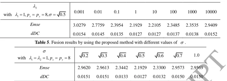
Table 4. Fusion results by using the proposed method with different values of 2.

2



with 11,pxpy8, 0.5

0.001 0.01 0.1 1 10 100 1000 10000

Emse 3.0279 2.7759 2.3954 2.1929 2.2105 2.3485 2.3535 2.9409

[image:22.595.93.489.109.250.2]

dDC 0.0154 0.0145 0.0135 0.0127 0.0127 0.0137 0.0138 0.0152

Table 5. Fusion results by using the proposed method with different values of .



with  1 21,pxpy8

0.2 0.3 0.4 0.5 0.6 0.7 1.0

Emse 2.9620 2.9613 2.3442 2.1929 2.3300 2.9573 2.9569

dDC 0.0151 0.0151 0.0133 0.0127 0.0132 0.0150 0.0150

Experimental results demonstrate that the fusion performance remains nearly unchanged when the

parameter ₁ is within the range of [0.001, 300]. When ₁ is larger than 300, the fusion performance

will be greatly degraded. In contrast, the fusion performance varies continuously with the parameter

2

 and is best when ₂ is set to 1, which is shown in the Table 4. As shown in Table 5, the fusion

performance also varies with the parameter  and achieves the best when  is set to 0.5 . Similar to those in the traditional SR and RSR fusion methods, better fusion results can be obtained

when the sizes of image patches are set to 8 8 . Therefore, we will set px py 8, 121 and

0.5

  in the following experiments.

5.3 Validity of the proposed fusion method

Several pairs of multi-focus images from two public databases are employed to thoroughly

demonstrate the validity of the proposed fusion method LR_RSR. Fig. 6 provides the ten pairs of

multi-focus images from the first database, which are downloaded from

http://home.ustc.edu.cn/~liuyu1. Fig. 7 illustrates the twenty pairs of multi-focus images from the

second database, which are downloaded from

https://www.researchgate.net/publication/291522937_Lytro_Multi-focus_Image_Dataset.

We will compare our proposed method LR_RSR with some state-of-the-art methods, including

SR [3], adaptive SR (ASR) [21], NSCT_SR [4], convolutional SR (CSR) [5], RSR [1], MRSR [1],

neighbor distance (ND) [12], NSCT [4], homogeneity similarity (HS) [35], image matting (IM) [36]

and deep convolutional neural network (DCNN) [37]. It should be noted that DCNN is a

deep-learning-based fusion method. The mutual information (MI) quality metric [38], gradient

ACCEPTED MANUSCRIPT

and the Q_PC metric [41] are employed to subjectively evaluate the different fusion methods. The

former two metrics MI and Q_G are used to evaluate the different fusion methods based on information

extraction, while the latter two metrics ZN_CC and Q_PC are used to evaluate different fusion methods

based on spatial consistency. Larger values of these metrics mean better fusion performance.

Fig. 6. Ten pairs of multi-focus images in the first database. The top row contains 10 input images with the focus on the left part,

and the bottom row contains the corresponding input images with the focus on the right part.

Fig. 7. Twenty pairs of multi-focus images in the second database. The first top row contains the first 10 input images with the

focus on the front part, and the second row contains the corresponding input images with the focus on the back part. The third row contains the remaining 10 input images with the focus on the front part, and the bottom row contains the corresponding input images with the focus on the back part.

Fig. 8 illustrates some fusion results on the first pair of multi-focus images in Fig. 6(a1) and Fig.

6(b1) (i.e., Fig. 5(a) and Fig. 5(b)) obtained by using different fusion methods. In order to better

compare different fusion methods visually, in Fig. 9, we also provide the normalized difference images

[1] between each of the fused images in Fig. 8 and one of the input images in Fig. 6(b1).

As shown in Fig. 8, all of the fusion methods mentioned here seem to perform well for Fig. 6(a1)

and Fig. 6(b1). However, a more careful comparison in Fig. 9 indicates that LR_RSR, DCNN and

MRSR perform better than others. As shown in Fig. 9(a) ~ Fig. 9(i), there are many residual errors

between each of the fused images and the input image Fig. 6(b1). This indicates that the fused images

obtained by these methods do not completely come from the focused regions of the input images and

thus introduce serious spatial artifacts, especially on the borders of the head of the student. In contrast,

ACCEPTED MANUSCRIPT

reduced. This demonstrates that MRSR, DCNN and our proposed LR_RSR method can more

accurately determine the focused and defocused regions of the input images. As shown in circle regions

of Fig. 9(j) ~ Fig. 9(l), few residual errors exist on the borders of head regions. This also indicates that

MRSR, DCNN and LR_RSR, especially the latter two methods, introduce fewer spatial artifacts to the

fused images.

Fig. 8. Fusion results for Fig. 6(a1) and (b1). (a) ND; (b) NSCT; (c) HS; (d) MF; (e) SR; (f) NSCT_SR; (g) ASR; (h) CSR; (i)

RSR; (j) MRSR; (k) DCNN; (l) LR_RSR.

Fig. 9. Normalized difference images between Fig. 6(b1) and each of the fused images in Fig. 8. (a) ND; (b) NSCT; (c) HS; (d)

MF; (e) SR; (f) NSCT_SR; (g) ASR; (h) CSR; (i) RSR; (j) MRSR; (k) DCNN; (l) LR_RSR.

Table 6. Performance of different SR-based fusion methods on the first database. Scores for the 10 image pairs in this database

are averaged.

Method MI QG ZNCC_PC QPC Tavg(s)

ND 3.9255 0.7438 0.9403 0.6541 2.0 NSCT 3.8461 0.7420 0.9458 0.6673 0.7 HS 4.8726 0.7629 0.9433 0.6858 0.8 MF 4.7915 0.7638 0.9597 0.6828 37.8

SR 4.5100 0.7583 0.9508 0.6793 15.9 NSCT_SR 4.0559 0.7496 0.9507 0.6735 12.6 ASR 3.7429 0.7244 0.8879 0.6321 42.0 CSR 4.0694 0.7396 0.9131 0.6656 43.1 RSR 4.7241 0.7707 0.9670 0.6977 880.1 MRSR 4.8530 0.7737 0.9686 0.7009 39.6 DCNN 4.8150 0.7681 0.9721 0.7005 43.8 LR_RSR 4.8127 0.7687 0.9752 0.6993 4.6

This visual comparison among different fusion methods is consistent with the quantitative results

in Table 6, which also demonstrates that MRSR, DCNN and LR_RSR perform better than other