Machine learning a general purpose interatomic potential for silicon

Machine Learning a General-Purpose Interatomic Potential for Silicon

Albert P. Bartók

Scientific Computing Department, Science and Technology Facilities Council, Rutherford Appleton Laboratory, Didcot, OX11 0QX, United Kingdom

James Kermode

Warwick Centre for Predictive Modelling, School of Engineering, University of Warwick, Coventry, CV4 7AL, United Kingdom

Noam Bernstein

Center for Materials Physics and Technology, U.S. Naval Research Laboratory, Washington, D.C. 20375, USA

Gábor Csányi

Engineering Laboratory, University of Cambridge, Trumpington Street, Cambridge, CB2 1PZ, United Kingdom

(Received 26 May 2018; revised manuscript received 11 October 2018; published 14 December 2018)

The success of first-principles electronic-structure calculation for predictive modeling in chemistry, solid-state physics, and materials science is constrained by the limitations on simulated length scales and timescales due to the computational cost and its scaling. Techniques based on machine-learning ideas for interpolating the Born-Oppenheimer potential energy surface without explicitly describing electrons have recently shown great promise, but accurately and efficiently fitting the physically relevant space of configurations remains a challenging goal. Here, we present a Gaussian approximation potential for silicon that achieves this milestone, accurately reproducing density-functional-theory reference results for a wide range of observable properties, including crystal, liquid, and amorphous bulk phases, as well as point, line, and plane defects. We demonstrate that this new potential enables calculations such as finite-temperature phase-boundary lines, self-diffusivity in the liquid, formation of the amorphous by slow quench, and dynamic brittle fracture, all of which are very expensive with a first-principles method. We show that the uncertainty quantification inherent to the Gaussian process regression framework gives a qualitative estimate of the potential’s accuracy for a given atomic configuration. The success of this model shows that it is indeed possible to create a useful machine-learning-based interatomic potential that comprehensively describes a material on the atomic scale and serves as a template for the development of such models in the future.

DOI:10.1103/PhysRevX.8.041048 Subject Areas: Computational Physics, Condensed Matter Physics, Materials Science

I. INTRODUCTION

A. Background

First-principles molecular simulation, based on various approximations of the electronic-structure theory, is the workhorse of materials modeling. For example, density-functional theory (DFT), a prominent method, is indicated

as the topic of about 19 000 papers published in 2017 according to the Web of Science database. However, because of the combination of its computational expense and unfavorable scaling, simulations that require thousands of atoms and/or millions of energy or force evaluations are carried out not using electronic-structure methods but empirical analytical potentials(also known asforce fields in the chemistry literature). These are parametrized approx-imations of the Born-Oppenheimer potential energy surface (PES), the electronic ground-state energy viewed as a function of the nuclear positions[1].

The functional form of analytical potentials is typically simple, based partly on a combination of physical and Published by the American Physical Society under the terms of

chemical intuition and partly on convenience. The param-eters are usually optimized so that the model reproduces, as best as it is able, either some macroscopic observables or microscopic quantities such as total energies and/or forces, corresponding to selected configurations and calcu-lated separately using an electronic-structure method. Unsurprisingly, while it is easy to find parameter sets that reproduce individual observables (e.g., the melting point corresponding to a particular composition or the binding energy of a crystalline structure), the simple functional forms postulated are not flexible enough to allow matching many properties simultaneously, and the potential energy surface is not accurate, which suggests that, when empirical analytical potentials are successful, there is a risk that this result is due to a fortuitous cancellation of errors and is then a case of getting the right answer for the wrong reasons. The practitioner is forced to select parameters subject to a trade-off between maximizing the accuracy for a few selected properties and transferability, i.e., avoiding a large or even qualitative error for a wide range of configurations and observables of interest [2,3]. This trade-off severely limits the predictive power of empirical analytical poten-tials when the very parameters that give sufficient accuracy for some known observables result in wildly varying predictions for new phases and properties whose prediction is the ultimate goal of the simulation.

Machine-learning (ML) methods provide a systematic approach to fitting functions in high-dimensional spaces without employing simply parametrized functional forms [4], thus opening up the possibility of creating interatomic potentials for materials with unprecedented accuracy for a wide range of configurations. The development in the past 10 yr required exploring a variety of ways to describe the chemical environment of atoms, the basis functions used to construct the potential, e.g., by various kernels or artificial neural network models, and the way such fits can be regularized, either by linear algebra or by various protocols of neural-network optimization[5,6]. The general approach is to define an atomic energy as a function of its local environment and fit this function in a 60–100-dimensional space corresponding to the relative positions of 20–30 nearby atoms. The challenge we take on here is to use this approach to develop ageneral-purposeinteratomic poten-tial, neither restricted to a narrow range of configurations or observables nor compromising accuracy in reproducing the reference potential energy surface. This approach requires adequately sampling enough of the space that is relevant to a wide range of atomistic simulations to interpolate it accu-rately and doing so in a computationally tractable manner.

The Achilles heel of machine-learning models, directly related to their flexibility, is their naturally much-reduced transferability: The flexible function representation is informed by a large training database, leading to a good fit for configurations near the database (in the space of the chosen representation) and progressively poorer away

from it. This limitation is often summarized by saying that high-dimensional fits are good at interpolation but less good at extrapolation, which can be viewed as another manifestation of the“curse of dimensionality”.

When first encountering the ML potential approach, one might wonder why such high-dimensional fits work at all, given that it is impractical to thoroughly sample the full space (e.g., on a grid). It is an empirical observation that they often do, so the real question is, what are the special properties of potential energy surfaces that make them amenable to such approximations? Regularity is almost certainly one of these, the mathematical concept encom-passing the colloquial idea of a potential varying smoothly as a function of the atomic positions. Indeed, the regular kernels that are used (and the corresponding regular activation functions in artificial neural networks) define the length scales over which predictions are interpolated rather than extrapolated. This definition can also point towards explaining why some methods work better than others: Kernels that better capture the inherent regularity of the underlying function interpolate better and extrapolate farther. Another property is that the configurations that are likely to arise in an atomistic simulation actually occupy a volume of configuration space that is much smaller than the full space. Consequently, a database derived from configurations found in reference atomistic simulations is sufficient for fitting an interatomic potential, so long as it includes not only the low-energy configurations but also nearby high-energy ones to constrain the potential at the boundary of the region that will be explored when it is used.

An obvious alternative approach to the transferability problem is to give up on it entirely and accept that an interatomic potential will always be extremely narrowly confined to its training database. One can then develop algorithms that activelyadapt or growthe training database during the course of a simulation [13–20]. The obvious disadvantage is that an electronic-structure method always has to be part of the simulation, to be called upon to calculate new target data as and when necessary. The efficacy of this approach then depends on what algorithm is used to detect that the simulation has strayed into parts of configuration space not sufficiently well covered by the current database and precisely what subsequent action is taken.

B. State of the art

The following is a brief review of the recent works in the emergent field of interatomic potential construction using high-dimensional nonparametric fits. Although fits to the potential energy surface of molecules and small molecule clusters have a much longer history[21–34], here we limit our scope to include only efforts that model strongly bound materials in the condensed phase. On the one hand, material models generally have a number of critical requirements that differentiate them from molecular models: (i) The potential must be reactive, i.e., needs to describe the forming and breaking of many covalent bonds, often simultaneously; (ii) a wide range of neighbor configurations need to be covered, including radical changes in neighbor count. Comprehensive models also need to (iii) cover multiple phases, e.g., metallic and insulating, solid and liquid, etc. On the other hand, many works cited below (and the present work) consider only one type of element, which allows the consideration of only relatively short-range interactions, because the absence of charge transfer obviates the need to describe long-range electrostatic effects.

Modeling the short-range interactions with artificial neural networks (NNs) really took off about a decade ago[35], starting with the bulk phases of silicon[36,37], with many more to follow: describing some silicon defects [38], the graphite-diamond transition[39], bulk zinc oxide [40], copper with some defects [41], the phase-change material GeTe in its various phases [42], various ionic solids[43,44], Li-Si alloys[45–47], bulk TiO₂[48], alloys [49,50], Ta₂O₅ [51], Li₃PO₄ [52], gold clusters [53], graphene [54], and various surfaces [55–59]. Fitting NN potentials is beginning to be combined with the combina-torial structure search [60–62].

Kernel fitting is a different approach to high-dimensional interpolation, with origins in statistics [cf. kriging[63]and Gaussian process regression (GPR) [64]] and widely applied in numerical analysis and machine learning [65]. The key to its success is the choice of kernel and, through it, the basis functions employed. In the context of atomistic potentials, a significant step was the introduction of rota-tionally and permutarota-tionally invariant representations that

also vary smoothly with the coordination number, based on the spherical Fourier transform and the bispectrum con-structed from it [66]. This representation was later sim-plified to the SOAP representation and kernel [7] and applied to tungsten[67], amorphous carbon [11,68], iron [69], graphene [12], and boron [70]. Using the original spherical bispectrum as a representation, potentials were made with linear regression for tantalum[71]and molyb-denum[72], with quadratic regression for tantalum [73], and with a nonlinear kernel for bulk Li₂B₁₂H₁₂[74]. Linear regression using yet another class of basis functions was introduced by Shapeev[75]and used to make a potential for Li[76]. Others use GPR with different representations to fit forces directly without constructing a potential, starting with a test for silicon[13], and more comprehen-sive models for aluminum[77–80].

Machine-learning methods and novel molecular repre-sentations and descriptors are also used for other regression tasks for molecules, using a variety of approaches to predict, e.g., atomization energies, atomic charges, NMR shifts, etc., [81–98], constructing molecular force fields[99–106], and even in combination with quantum mechanics/molecular mechanics (QM/MM) embedding methods[107].

C. A general potential

Here, we demonstrate that, using ML techniques, it is indeed possible to develop an accurate potential that spans a wide range of physically important structures and proper-ties. Using silicon as an example, we create a potential and demand that it give reasonably accurate predictions for all configurations relevant to scientific questions within a wide temperature and pressure range, including surfaces, point and line defects, cracks, etc. Silicon is a good material for such a study for a number of reasons. First, it has a rich phase diagram with many stable and metastable crystal structures, as well as a wide variety of point and line defects and surface reconstructions. Second, the simulation com-munity has extensive experience in understanding many aspects of its potential energy surface. Finally, there are a large number of empirical analytical potentials that have been constructed over the past decades whose successes and failures give a detailed picture of what it is about the potential energy surface that is relatively easy to get right and what the more difficult aspects are.

e.g., using the DFT to study the 7×7 dimer-adatom-stacking-fault reconstruction of the Si (111) surface[113]. Silicon is also extensively used as a model system to understand fracture and, in particular, the interplay between brittle and ductile failure[114–118].

A large number of interatomic potentials have been developed for silicon with the intent of describing its bulk phases and defects. While there are too many publications to thoroughly review here, we discuss the most widely used and successful ones, to motivate our choices for compari-son models in this work. By far the two most commonly used are those of Stillinger and Weber (SW)[119,120]and Tersoff [2,121–124]. Both include pair terms and three-body terms, the former defined in terms of bond lengths and bond angles, the latter in terms of a repulsive core and a bond-order-dependent attractive bonding interaction. Many other functional forms are also used, as reviewed, e.g., by Balamane, Halicioglu, and Tiller[125]and more recently by Purja Pun and Mishin [126]. While none produce sufficient improvement to lead to a significant adoption by the simulation community, recent attempts to add terms that depend on more than three-body interactions have been at least somewhat successful. These include the environ-ment-dependent interatomic potential (EDIP)[127], modi-fied embedded atom method (MEAM)[128,129], ReaxFF [115,130], and screened Tersoff [131,132]. EDIP uses the local coordination of each atom to approximate a bond order (a chemical concept that is also integral to the Tersoff potential) and change the preferred bond length, strength, and bond angle correspondingly. MEAM is an angle-dependent functional form that evolved out of the simpler embedded atom method, mainly used for metals. It was first applied to silicon with a first-neighbor cutoff distance by Baskes, Nelson, and Wright[133]and later reparametrized several times with different choices of fitting quantities and interaction cutoffs[129,134,135]. Here, we use the second-neighbor cutoff parametrization due to Lenosky et al. [129]. The ReaxFF form was originally developed in the context of computational chemistry to describe reactions of molecules, and the silicon potential we use [130] was previously used to simulate a brittle fracture [115]. The screened Tersoff form (TersoffScr) was developed by Pastewkaet al., who modified the Tersoff functional form with a screening term to improve its performance for fracture properties [131,132], where bonds are broken and formed. Finally, Purja Pun and Mishin took the modified Tersoff form developed by Kumagai et al. [136] and optimized it for a wide range of properties [126]. We compare the results of GAP to these interatomic potential models (EDIP, MEAM, Purja Pun, ReaxFF, SW, Tersoff, and TersoffScr) and also to the density-functional tight-binding (DFTB) method [137–139].

The inclusion of a tight-binding (TB) model in the above list is essential, because TB represents a middle ground between the DFT and interatomic potentials. The TB

approach is a minimal description of electronic structure [1], significantly cheaper than the DFT, yet still carrying the essentially quantum-mechanical nature of the electrons, giving a qualitatively robust description of their behavior in solids in a wide range of materials. Like interatomic potential models, TB can be easily implemented with a cost that is linear in the number of atoms. A lot of effort has gone into making accurate TB models[138,140–150], and, if they were clearly more accurate or transferable than conventional interatomic potentials, they might present the same trade-off between speed and accuracy as ML models, which are also significantly more computationally expen-sive than conventional interatomic potentials. However, such does not appear to be the case: The widely used TB model included here does not perform better on the whole than analytical potentials. For the DFTB calcula-tions, we use the“pbc”parameter set and ak-point density of 0.007Å−1 for bulk configurations and 0.04Å−1 for others. To reduce the computational cost, no charge-self-consistency iterations are performed, since they are not expected to lead to substantial differences for this monatomic covalently bonded material.

Our focus is on creatingusefulmodels, and therefore the guiding principle is to create a data set and fitting protocol that is theleastspecific to the material and the observables as possible while still achieving the aims. On the one hand, we try to create tests that are as relevant to the materials modeler as possible, focusing on observables that are either directly comparable to experiments or at least generally agreed to be important for the understanding of material behavior. On the other hand, we think of the ML potential as an interpolation scheme for the reference DFT method, so, with a few exceptions, we compare the interatomic potential results to the DFT, rather than to an experiment, for example.

It is worth noting that the comparisons with analytical potentials we show in this paper are not meant as a definitive evaluation of their accuracy. Since the analytical potentials are fit to different sets of properties from different sources, their performance for any particular observable could very well be improved somewhat by refitting them to our DFT data; we do not see the relevance of doing that here and work with the published parametrizations, since the analytical potentials’ main advantages are simplicity, computational efficiency, and some transferability rather than ultimate accuracy. In the case of a machine-learned model, the unique selling point is the accuracy with which the target potential energy surface is matched, which is best demonstrated by comparing to DFT results. The route to an improved agreement with experimental observables is to improve the target, i.e., using a more accurate description of the electronic structure.

set into training, testing, and validation. This is partly because this has been done many times before for the same kernel, representation, and approach to parameter choice that we use here and partly because the SOAP kernel does not have hyperparameters that are worth optimizing: They are dictated by the length and energy scales inherent in atomic interactions, which are well known. (The other parameters in the regression correspond to accuracy targets on a few classes of configurations.) Ultimately, the paper is about the validation on material properties, and all those are based on atomic configurations which are themselves not in the training set.

Figure1provides an overview of many of the verifica-tion and validaverifica-tion tests carried out for our new silicon

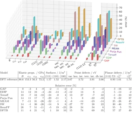
GAP model in comparison to the empirical analytical models mentioned above. While the individual tests are discussed in more detail below, we present an overview here. The first three groups of quantities in the figure are verification tests, in the sense that they require accuracy on configurations which are directly represented in the training set. These are split into three classes of test: bulk properties, surfaces, and point defects. Bulk properties, namely, the bulk modulusB and diamond cubic elastic constantsC₁₁, C₁₂, andC₄₄, are well reproduced by the GAP model with fractional errors relative to the DFT of less than 10%; none of the other interatomic potentials reach this accuracy, although in many cases they are fit to different training data (e.g., an experiment or simply other exchange-correlation

FIG. 1. Comparison of percentage errors made by a range of interatomic potentials for selected properties, with respect to our DFT reference. Those on the left of the break in the axis are interpolative, i.e., well represented within a training set of the GAP model: elastic constants (bulk modulusB, stiffness tensor componentsCij), unreconstructed (but relaxed) surface energies [(111), (110), and (100)

functionals). The largest relative errors in bulk properties are typically made in the softest elastic constantC₁₂, with the EDIP model being the next most accurate after our new GAP model. The second class of verification tests dem-onstrates that the GAP model performs consistently at describing surface energies of the (111), (110), and (100) cleavage planes, with errors of around 2% with respect to our reference DFT calculations. Here, the scatter across the various other models is smaller than for bulk properties. For example, the (100) surface energy is, in general, well described by most models. For the third class of verification tests, formation energies of vacancy and interstitial point defects, we see a wide range of errors across the models evaluated. The new GAP model again predicts all these quantities within 10% of the reference DFT results. In general, for any particular property, there is often a model that provides an accurate description, but apart from the GAP, we are not aware of any model that provides uniform accuracy across the whole range of properties in Fig.1. The typical spread between DFT exchange-correlation func-tionals for structural and vibrational properties of silicon is much smaller; e.g., Ref. [151]reports only around a 1% variation in Si lattice constants and fundamental phonon frequencies over a wide range of exchange-correlation functionals.

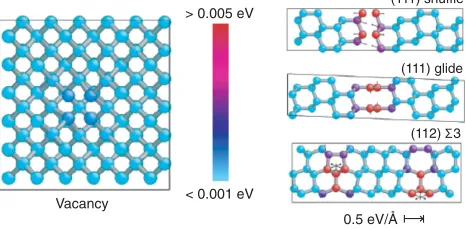
Moving to more stringent tests of the new model, we consider a set of planar defects which are not represented in the training set (right-hand group in Fig. 1), namely, the

ð112ÞΣ3 symmetric tilt grain boundary, and unstable stacking-fault energies on the (111) shuffle plane γðussÞ

and (111) glide plane γðusgÞ. For these tests, the accuracy

of the GAP model is reduced but still within 20% of the DFT, comparing favorably with all other models, some of which include stacking-fault values in their training sets (e.g., EDIP). Moreover, the ability of the GAP model to provide an estimated error along with its predictions allows us to qualitatively assess the expected reliability of the model for particular classes of configurations. Figure 2

shows the predicted errors for each atom in the vacancy, shuffle, glide, and grain boundary configurations. For the vacancy, the confidence of the model is high on all atoms (blue), and the corresponding accuracy with respect to DFT is high. The reduced confidence close to the planar defects (red atoms) is consistent with the larger errors made for these configurations and the fact that the database does not include any similar atomic environments.

The rest of the paper is organized as follows. In Sec.II, we give an overview of the potential fitting methodology and the construction of the database. In Sec.III, we report on extensive tests that serve to verify that those properties which the database is explicitly designed to capture are indeed correctly predicted. This testing includes equations of state, average structural properties of liquid and amor-phous states, point-defect energetics, surface reconstruc-tions, and crack-tip geometries. In Sec.IV, we validate the model by showing predictions for properties that are deemed fundamental for modeling this material but for which the database makes no special provision. These predictions includes thermal expansion, di-interstitials, grain boundaries, and random structure search. We finally give a brief outlook in Sec.V.

II. METHODOLOGY

A. Potential fitting

The interatomic potential, even after assuming a finite interaction radius, is a relatively high dimensional func-tion, with dozens of atoms affecting the energy and force on any given atom at the levels of tolerances we are interested in (around a meV per atom). However, much of the interaction energy (in absolute magnitude) is captured by a simple pair potential, describing exchange repulsion of atoms at close approach and potentially the chemical bonding in an average sense farther out. In anticipation of the kernel approach for fitting the inter-atomic potential, the pair potential also serves a useful purpose from the numerical-efficiency point of view, because the exchange repulsion it takes care of is a component of the potential that is very steep, in com-parison with the bonding region, and such disparate energy scales are difficult to capture with a single kernel in high dimensions.

In the present case, we choose a purely repulsive pair potential, given by cubic splines that are fitted to the interaction of a pair of Si atoms, computed using DFT. This choice leaves the description of the attractive part entirely for the many-body kernel fit.

We start by giving a concise account of the GAP kernel-fitting approach, as we use it here. The total GAP model energy for our system is a sum of the predefined pair potential and a many-body term which is given by a linear sum over kernel basis functions[64]:

> 0.005 eV

< 0.001 eV

(111) shuffle

0.5 eV/Å (111) glide

(112) 3

Vacancy

E¼X i<j

Vð2ÞðrijÞ þ

X

i

XM

s

αsKðRi;RsÞ; ð1Þ

whereiandjrange over the number of atoms in the system, Vð2Þis the pair potential,rijis the distance between atomsi andj,Kis a kernel basis function defined below, andRiis the collection of relative position vectors corresponding to the neighbors of atomiwhich we call aneighborhood. The last sum runs over a set ofMrepresentativeatoms, selected from the input data set, whose environments are chosen to serve as a basis in which the potential is expanded (more on this below).

The value of the kernel quantifies the similarity between neighborhoods (in the Gaussian process literature, it is a covariance between values of the unknown function at different locations), which is largest when its two argu-ments are equal and smallest for maximally different configurations. The degree to which the kernel is able to capture the variation of the energy with the neighbor configuration determines how efficient the above fit is. The better the correspondence, the fewer representative configurations are needed to achieve a given accuracy. It also helps tremendously if exact symmetries of the function to be fitted are already built into the form of the kernel. For an interatomic potential, we need a kernel that is invariant with respect to the permutation of like atoms and 3D rotations of the atomic neighborhood. Note that translational invariance is already built in, because the kernel fit is applied to each atom individually—this very natural decomposition of the total energy is customary when fitting interatomic potentials and is directly analo-gous with the spatial decomposition of convolutional neural networks[152].

Here, we use the SOAP kernel [7,8]. We start by representing the neighborhoodRiof atomiby itsneighbor density,

ρiðrÞ ¼

X

i0

fcutðrii0Þe−ðr−rii0Þ=2σ 2

atom; ð2Þ

where the sum ranges over the neighbors i0 of atom i (including itself), fcut is a cutoff function that smoothly

goes to zero beyond a cutoff radius rcut, and σatom is a

smearing parameter, typically 0.5 Å. Invariance to rotations is achieved by constructing a Haar integral over the SO(3) rotation group[7]. The SOAP kernel between two neighbor environments is the integrated overlap of the neighbor densities, squared, and then also integrated over all possible 3D rotations:

˜

KðRi;RjÞ ¼

Z

ˆ R∈SOð3Þ

dRˆ

Z

drρiðrÞρjðRˆrÞ

2: ð3Þ

To obtain the final kernel, we normalize and raise to a small integer power:

KðRi;RjÞ ¼δ2

˜

KðRi;RjÞ

ffiffiffiffiffiffiffiffiffiffiffiffiffiffiffiffiffiffiffiffiffiffiffiffiffiffiffiffiffiffiffiffiffiffiffiffiffiffiffiffiffi ˜

KðRi;RiÞK˜ðRj;RjÞ

q ζ

ð4Þ

with ζ¼4 in the present case. The δ hyperparameter corresponds to the energy scale of the many-body term, and we useδ¼3eV, commensurate with typical atomization energy per atom. The accuracy of the fit is not particularly sensitive to this parameter.

In practice, we do not evaluate the above integrals directly but expand the neighbor density in a basis of spherical harmonicsYlmðˆrÞand radial functionsgnðrÞ(we use equispaced Gaussians, but the formalism works with any radial basis):

ρiðrÞ ¼

X

nlm ci

nlmYlmðrˆÞgnðrÞ: ð5Þ

The following spherical power spectrum vector (henceforth termed the “SOAP vector”) is a unique rotationally and permutationally invariant description of the neighbor envi-ronment,

˜ pi

nn0l¼

Xl

m¼−l ci

nlmcin0lm ð6Þ

pi_¼p˜i_=jp˜i_{j; ð7Þ}

and the SOAP kernel can be written as its scalar product:

KðRi;RjÞ ¼δ2jpi·pjjζ: ð8Þ

The coefficientsαsin Eq.(1)are determined by solving a linear system that is obtained when available data are substituted into the equation, as we detail below. In the present case, these data take the form of total energies and gradients (forces and stresses) corresponding to small- and medium-sized periodic unit cells, calculated using the density-functional theory.

There are two factors that complicate the determination of the vector of linear expansion coefficients,α. The first is that atomic energies are not directly available from the density-functional theory, and the second is the presence of gradients in the input data. The following treatment addresses both of these. We denote the number of atoms in the input database with N and define _y as the vector with D components containing the input data—all total energies, forces, and virial stress components in the training database—_y0 as the vector withN components containing theunknownatomic energies of theNatomic environments in the database, andLas the linear differential operator of size N×D which connects _y with _y0 such that _y¼L_y0. After selectingMrepresentative atomic environments (with M≪N), the regularized least-squares solution for the coefficients in Eq. (1)is given by [156,157]

α_¼½K

MMþðLKNMÞTΛ−1LKNM−1ðLKNMÞTΛ−1y; ð9Þ

where KMM is the kernel matrix corresponding to the M representative atomic environments [with matrix elements from Eq.(8)], K_NM is the kernel matrix corresponding to the representative set and all of theN environments in the training data, and the elements of the diagonal matrixΛ−1 represent weights for the input data values. The Bayesian interpretation of the inverse weights is expected errors in the fitted quantities. While takingΛ¼σ2_νIwith an empiri-cal value forσ_νwould be sufficient to carry out the fit, this interpretation makes it straightforward to set sensible values. The expected errors are not just due to a lack of numerical convergence in the electronic-structure calcula-tions but also include the model error of the GAP representation, e.g., due to the finite cutoff of the local environment. Our informed choices for these parameters are reported in Table I.

For several systems below, we include results on the predicted error, the measure of uncertainty intrinsic to our interpolated potential energy surface. These come from the Bayesian view of the above regression procedure, in which the data (and the predicted values) are viewed as samples from a Gaussian process whose covariance function is the chosen kernel function [64]. The mean of this Gaussian process is, of course, just the second term of the predicted energy, Eq. (1), and the predicted variance of the atomic energy for atom i is given by

KðRi;RiÞ−kT_ðK

MMþσeIÞ−1k; ð10Þ

where the elementsof the vectorkis given byKðRi;RsÞ, the covariance between the environment of atomiand the environments of the representative atomssin the database. The above is a simplified error estimate, in which we regularize using the parameterσe, typically set to 1 meV [equal to the value used for the per-atom energy data

components ofΛfor most of the database in Eq.(9)] rather than using the more complicated regularization as in Eq. (9). We interpret this variance as the (square of the)

“one-sigma” error bar for the atomic energies.

B. Database

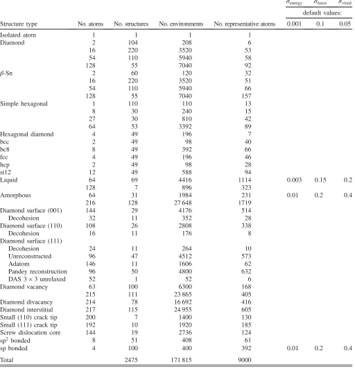
The database of atomic configurations (periodic unit cells) is described in TableI. It was built over an extended period, using multiple computational facilities. The kinds of configuration that we include are chosen using intuition and past experience to guide what needs to be included to obtain good coverage pertaining to a range of properties. The number of configurations in the final database is a result of somewhat ad hoc choices, driven partly by the varying computational cost of the electronic-structure calculation and partly by observed success in predicting properties, signaling a sufficient amount of data. Each configuration yields a total energy, six components of the stress tensor, and three force components for each atom. The database there-fore has a total of 531 710 pieces of electronic-structure data. We represent the diversity of atomic neighborhoods using M¼9000representatives [see Eq.(1)], and the number of these picked from each of the structure types by the CUR algorithm is also shown in the table.

We use the CASTEP software package [158] as our

density-functional-theory implementation, and manual cross-checking is done to ensure that the calculations are consistent between different computers. The main param-eters of the electronic-structure calculation are as follows: PW91[159]exchange-correlation functional (the choice is motivated by the existence of a large-scale simulation of the melting point with this functional), 250 eV plane-wave cutoff (with finite basis corrections), Monkhorst-Pack k-point grids with 0.03Å−1 spacing (corresponding to a 603 _{grid in the primitive cell), ultrasoft pseudopotentials,}

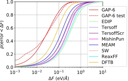
force errors than any other potential tested, with a median of about0.025eV=Å, an order of magnitude smaller than for the analytical potentials. The testing database, which consists of a grain boundary, six di-interstitials, the unre-laxed and reunre-laxed shuffle and glide generalized

stacking-fault paths, and an amorphous configuration, shows a very similar distribution of the force error, although the actual errors are strongly dependent on the type of geometry, so changing the proportions of each could change the resulting distribution somewhat.

TABLE I. Summary of the database for the silicon model. The first column shows the number of atoms in the periodic unit cells, and the second column shows the number of such unit cells in the database, while the third column is the product of the first two and, thus, shows the number of atoms (and, therefore, atomic environments) in the database for each structure type. The fourth column shows the number of representative atoms picked automatically from each structure type by the CUR algorithm (see the text). The last three columns show the regularization we use in the linear system (empty rows correspond to using the defaults, given at the top).

σenergy σforce σvirial default values:

Structure type No. atoms No. structures No. environments No. representative atoms 0.001 0.1 0.05

Isolated atom 1 1 1 1

Diamond 2 104 208 6

16 220 3520 53

54 110 5940 58

128 55 7040 92

β-Sn 2 60 120 32

16 220 3520 51

54 110 5940 66

128 55 7040 157

Simple hexagonal 1 110 110 13

8 30 240 15

27 30 810 42

64 53 3392 89

Hexagonal diamond 4 49 196 7

bcc 2 49 98 40

bc8 8 49 392 66

fcc 4 49 196 46

hcp 2 49 98 28

st12 12 49 588 94

Liquid 64 69 4416 1114 0.003 0.15 0.2

128 7 896 323

Amorphous 64 31 1984 231 0.01 0.2 0.4

216 128 27 648 1719

Diamond surface (001) 144 29 4176 514

Decohesion 32 11 352 28

Diamond surface (110) 108 26 2808 338

Decohesion 16 11 176 8

Diamond surface (111)

Decohesion 24 11 264 10

Unreconstructed 96 47 4512 573

Adatom 146 11 1606 62

Pandey reconstruction 96 50 4800 632

DAS3×3unrelaxed 52 1 52 6

Diamond vacancy 63 100 6300 168

215 111 23 865 405

Diamond divacancy 214 78 16 692 416

Diamond interstitial 217 115 24 955 605

Small (110) crack tip 200 7 1400 130

Small (111) crack tip 192 10 1920 185

Screw dislocation core 144 19 2736 124

sp2bonded 8 51 408 61

sp bonded 4 100 400 392 0.01 0.2 0.4

Note that the testing database for Fig.3is not the result of the usual random split into training and test sets but represents extrapolation into configurations entirely differ-ent from those in the training database, providing an even more stringent test than the usual split. Since the empirical analytical potentials are not fit to our database, the latter serves as a test for the potentials. It is remarkable how good the analytical potentials’ predictions are for macroscopic properties, which are mostly energy differences, given the large force errors shown here.

C. Convergence

Since the principal goal of machine-learned interatomic potentials is to enable the prediction material properties by fitting the Born-Oppenheimer potential energy surface, it is interesting to consider theconvergenceof such a potential. The expectation is that a closer match of the potential energy surface will result in more accurate predictions. While a comprehensive convergence study is beyond the scope of this work, there are simple convergence

parameters in the SOAP-GAP framework that directly control the trade-off between computational cost and accuracy of the fit. One is the numberMof representative environments (effectively the number of basis functions in the regression), and the other is the truncation of the spherical harmonic and radial basis expansion of the atomic neighbor density [Eq.(5)]. Figure4shows the convergence of the SOAP or GAP model with respect to these. We use theΔvalue of Lejaeghereet al.[162]to compute the error in the energy-volume curves for diamond andβ-Sn with respect to our DFT reference, defined as

Δ¼

ffiffiffiffiffiffiffiffiffiffiffiffiffiffiffiffiffiffiffiffiffiffiffiffiffiffiffiffiffiffiffiffiffiffiffiffiffiffiffiffiffiffiffiffiffiffiffiffiffiffiffiffiffiffiffiffiffiffiffiffiffiffiffiffi R_1.06V0

0.94V0 ½E

GAP_ðVÞ−EDFT_ðVÞ2_dV

0.12V₀

s

;

where EGAP and EDFT denote GAP and DFT energies, respectively, relative to the diamond energy minimum to allow comparison,V₀is the DFT minimum-energy volume for each phase, and the integral is computed numerically by fitting cubic splines to 12 ðE; VÞ pairs for each model. Good convergence can be seen with respect to both basis set size and the accuracy of the expansion of the atomic density, with a precision of the order of a meV (forβ-Sn; for diamond, another order of magnitude better), indicating that GAP reproduces the target DFT energy surface better than the typical variability between DFT codes of the order ofΔ¼1meV reported in Ref. [162].

In principle, a Gaussian process regression model should be able to converge to a given target function with arbitrary accuracy as the database size grows. However, in this case, the only remaining physical approximation is the finite cutoff of the interatomic potential, which means that the force on an atom that is computed using our DFT engine is not strictly a function of the finite neighborhood of the atom. From the point of view of a model with a finite cutoff, the target function appears to have an finite amount of uncertainty, and this uncertainty is taken into account when TABLE II. Coordination statistics ci (fraction of atoms with number of neighbors i within rc¼2.75Å, in

percent) and energy per atom relative to the diamond structure (ΔEac, in eV) for amorphous structures resulting from quenching of the liquid. The energy difference evaluated using the interatomic potential isΔIP_{ac, the energy difference} of the interatomic-potential-relaxed structure evaluated (but not relaxed) using the DFT isΔEeD

ac, and the DFT-evaluated energy difference of the DFT-relaxed structure starting from the interatomic potential structure isΔErD

ac. Most atoms in the MEAM structure have coordination≥6. The experimental defect density is from Ref.[160]and the energy from Ref.[161].

Model c₃ c₄ c_{5 Δ}EIP

ac ΔEeDac ΔErDac

Lit. exper. ≥99 0.137

GAP 1.4 98.1 0.5 0.15 0.14 0.13

EDIP 0.5 94.4 5.1 0.22 0.22 0.19

Tersoff 0.0 98.1 1.9 0.22 0.18 0.17

MEAM 0.0 0.0 2.8 0.14 0.65 0.28

SW 2.3 75.5 21.8 0.20 0.29 0.23

ReaxFF 0.0 86.1 13.9 0.35 0.35 0.25

fitting the model, as mentioned above. Indeed, previous investigations show that, with a cutoff of 5 Å, an error of 0.1eV=Å on the forces is about what is to be expected for the diamond structure[163–165]. Note that it is possible to estimate the expected force error due to the finite cutoff directly from the DFT engine, because forces are them-selves local quantities, as opposed to site energies and virial stress components, which are not observable directly.

It is noteworthy how much more accurate the potential is for the diamond structure than for β-Sn. Two factors contribute to this: First, there are many more diamondlike configurations in the database, particularly the configura-tions associated with various defects, and, second, the locality error is expected to be significantly larger for the β-Sn structure due to its metallic electron density of states. Small clusters represent a class of systems where locality is even worse, due to delocalized surface states and a fluctuating Fermi level, whose effects decay slowly with the inverse of the system size[166]. The type of bonding in small clusters varies wildly as the cluster size changes, with reactive, metallic ground states and inert, closed-shell

“magic number” clusters competing energetically [167– 169]. This variation suggests that interatomic potentials in general are not well suited to accurately model silicon clusters; hence, we decide to omit them from this study.

We do not claim that our database in the present work is complete in a mathematical sense (even within the restric-tion of the given cutoff) but that, for any particular application whose relevant configurations are well repre-sented in the database, errors can be improved only by choosing a larger cutoff, which in turn might lead to the need to enlarge the database further.

D. Testing

A software testing framework was built to run tests of the potential using the atomic simulation environment (ASE) [170]. Each model and test is implemented as an indepen-dent PYTHONmodule, allowing all tests to be run with each

model (similarly to the design of the OpenKIM project [171]). The model modules are simple, consisting of calls to existing ASE interfaces to QUIP [172] (GAP, DFTB, Stillinger-Weber, Tersoff, and MEAM), LAMMPS [173] (EDIP, Purja Pun, and ReaxFF), and ATOMISTICA [174] (TersoffScr). Reference DFT results are obtained using the same tests with a model based on the ASE interface to Castep and using the parameters discussed above. One advantage of this automated approach is that it ensures consistency in starting configurations, minimization algo-rithms, and the final test results that are shown in our figures. Another is that it enables automated rerunning of tests when changes are made, e.g., to the GAP training database, allowing incremental improvements to be assessed. The framework is available for download[175].

III. RESULTS: VERIFICATION

In this section, we report on a series of basic tests which the GAP model is designed to pass, because they corre-spond to configurations that are selected for inclusion in the database for the purpose of describing those very observ-ables. We refer to these as“verification,”by analogy to the usage of the term in software engineering, where it refers to the confirmation that the software implements the speci-fications correctly.

corresponding models) will never be deemed completely final and definitive. By designating some tests as part of

“verification,”we mean to be open about the fact that the database is amended qualitatively and quantitatively until these tests are passed to our satisfaction, and, therefore, these tests are in some sense merely the achievement of a good fit. In the following “validation” section (again by analogy to the use of the term in software engineering where it refers to the confirmation that the specifications describe a method that achieves the desired goal), we collect tests for which the database is not explicitly designed but concern observables that a good model for the material ought to be able to describe. We make no attempt to augment or modify the database in order to improve the results of those tests, and this could, and indeed should, be done in future work.

A. Bulk crystals

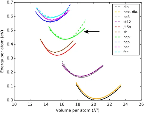
As an initial test, we calculate the energy vs volume for a number of bulk crystal structures for silicon, including the ground-state diamond structure, closely related hexagonal diamond, known high-pressure structures β-Sn, simple hexagonal (sh), bc8, and st12 structures, as well as even higher pressure phases, hexagonal close packed (hcp), body-centered cubic (bcc), and face-centered cubic (fcc). When calculating these curves with the DFT as well as DFTB and each interatomic potential, we deform the lattice to the target volume and relax it with respect to the unit cell shape and atomic position while approximately con-straining the volume and also concon-straining the symmetry (using spglib [176]) to remain that of the initial structure.

We find that the hcp structure has two minima, the conventional one withc=a≈pffiffiffiffiffiffiffiffi3=2 and another we label hcp0, which has a much lowerc=a <1.

The resulting EðVÞ curves for each crystal structure calculated with the GAP and compared to our reference DFT calculations are shown in Fig. 5. The results are in excellent agreement for all structures tested, including minima positions (volume), depths (cohesive energy rela-tive to the ground state), and curvatures (bulk modulus). The hcp0structure, which is not in the fitting database, has a larger discrepancy than the other structures, although it is still in good agreement. A comparison of all the models for a few selected crystal lattices (diamond structure,β-Sn, and fcc) is shown in Fig.6. Only the GAP is even qualitatively reproducing all three selected structures, and many of the models fail to reproduce even the first structure seen experimentally under applied pressure,β-Sn.

FIG. 5. Energy per atom vs volume per atom for various bulk crystal lattice structures computed using the DFT (solid lines) and GAP (dashed lines). The hcp0structure (indicated by an arrow), which is not in the fitting database, has a substantially larger discrepancy between the DFT and GAP than any of the other structures, all of which are in the database.

B. Liquid

To simulate the structure of liquid silicon with each interatomic potential and DFTB, we use constant-pressure (P¼0GPa) molecular dynamics as implemented in the QUIP package through the quippy PYTHONinterface[172].

A2×2×2supercell of the eight-atom diamond cubic cell (64 atoms total) is heated fromT¼0K toT ¼5000K for rapid melting over 20 000 0.5 fs time steps and then equilibrated at T¼2000K for 10 000 0.25 fs time steps. Structural data are gathered over an additional 5000 0.25 fs time steps. Reference DFT results are obtained from a similar MD simulation using the Castep software, averag-ing over 9700 0.25 fs time steps at T¼2000K. For the electronic-structure calculations, a 200 eV plane-wave energy cutoff and a 2×2×2 Monkhorst-Pack [177] k-point grid are used (equivalent to a k-point density of about 0.05Å−1). The radial distribution function (RDF) and angular distribution function (ADF) are calculated and averaged using the tools included in QUIP.

The resulting structural quantities are shown in Fig. 7. The GAP RDF is in excellent agreement with the DFT result, including both peak heights and radii at all distances captured in the simulation cell. The DFTB is in comparably good agreement on this structural quantity, and the various interatomic potentials are in much worse agreement, with significant variation among them. The ADF proves to be an even more stringent test. Again, the GAP results are in excellent agreement with the DFT, showing a narrow peak at about 60° and a broader peak with similar height at about 100°. Most of the potentials greatly underestimate the height of the small-angle peak and overestimate the height of the large-angle peak. The only two that are qualitatively correct are EDIP and MEAM, but those both overestimate the depth of the trough separating the two peaks. Several issues with the analytical interatomic potentials may be the source of the differences. Some, e.g., Tersoff [2], greatly overestimate the melting point and are therefore strongly undercooled at T¼2000K rather than an equilibrium liquid. In other cases, it is possible that the wide variety of curves observed is consistent with the hypothesized liquid-liquid phase transition between a coordination, high-density metallic phase and a low-coordination, low-high-density semiconductorlike phase[178]. Some of the potentials may simply be incorrectly predicting the low-coordination phase to be present atT¼2000 K and zero pressure, leading to a predominantly tetrahedral-like bond angle distribution.

In addition to the two structural quantities, we evaluate a dynamical quantity, the diffusivity of liquid Si, by carrying out variable cell size constant enthalpy MD simulations using the LAMMPS software [173,179] on a 512-atom cell for 105 1 fs time steps at temperatures ranging from about 1700 to 2200 K. The resulting diffusivity as a function of the temperature is shown in Fig. 8 and compared to the experimental results [180], DFT results [181](using the PBE generalized gradient approximation

exchange-correlation functional, which is somewhat differ-ent from the PW91 functional we use to generate our fitting database), and previously published SW potential results [182–185]. The GAP results are in excellent agreement FIG. 7. Liquid silicon radial and angular structure from well-equilibrated constant temperature and pressure 64-atom samples atP¼0GPa andT¼2000K. Top: RDF. Bottom: ADF. The black solid line indicates DFT results, the red dashed line and symbols indicate GAP results, and dashed lines (various colors) indicate the DFTB and other interatomic potentials.

with the DFT, and so both underestimate the experimental diffusivity. This difference relative to the experiment has previously been ascribed to the tendency for DFT to exaggerate the structure of the liquid [181], and so the similar diffusivities of the GAP and DFT are consistent with the similarities in their liquid RDF and ADF.

C. Amorphous phase

Amorphous silicon is an interesting tetrahedrally coor-dinated phase that forms upon various forms of processing, including ion implantation, low-temperature deposition, and rapid quenching from the melt. The last of these is commonly used in simulations, but it is challenging to reach experimentally relevant cooling rates using accurate methods such as the DFT. We therefore carry out zero-pressure variable cell volume (hydrostatic strain) simula-tions of the quenching of a 216-atom sample of liquid Si, cooled at1012 K=s from 2000 to 500 K with a 1 fs time step (1.5×106 steps) using the LAMMPS software, and then relax to the local energy minimum with respect to atomic positions and cell size and shape. The initial configuration for all quenches is from a GAP equilibrated liquid at T¼1800K, which is further equilibrated with each potential at T ¼2000K for an additional 105 time steps before cooling. As for the liquid above, for some potentials this initial thermodynamic state may be a strongly under-cooled liquid due to their overestimation of the melting temperature.

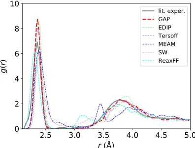
The RDFs of the resulting structures are shown in Fig.9, in comparison with experimental results[186](since DFT results for comparable sizes or quench rates are not computationally feasible). The various interatomic models vary widely in the overall shape of their RDF, with GAP, EDIP, and Tersoff in best agreement with the experiment, showing a sharp first neighbor peak at about 2.35 Å

and a broad second peak at about 3.8 Å. These three models have essentially no atoms between the two peaks (2.5Å≲r≲3.25Å). The other models show various qualitative problems, including smaller peaks between the two expected ones or an excess of atoms throughout the entire distance range between the first and second neighbor peaks. The corresponding coordination statistics (usingr¼2.75Å as the nearest-neighbor distance cutoff) are shown in TableII. The GAP and Tersoff models have the lowest coordination defect concentration, significantly lower than the next-best model, EDIP, and closest to the experimental estimates of ≤1% [160].

Table II also lists the amorphous-crystal energy differ-enceΔEac relative to the diamond structure. The obvious

way to evaluate the energy difference for each structure is to use the same interatomic potential that is used to generate the structure, i.e., a calculation that is entirely self-consistent for that potential. ThisΔEIP

ac listed in the table

shows the GAP with the closest value to the experiment [186] (excluding MEAM, which has a very unphysical structure), while other interatomic potentials result in higher energy differences. However, using the potential to evaluate the energy difference risks mixing up errors in the structure with errors in the energy difference given the structure, with the possibility of exaggerating or under-stating the stability of the amorphous structure, depending on the sign of the energy error. For an independent evaluation of the quality of the quenched a-Si structures, we evaluate their energies with the DFT (ΔEeD

ac) and also

further relax them with the DFT (ΔErD

ac). Note that these

calculations are done with a lower k-point density, 0.07Å−1, due to the computational expense of the 216-atom cells. In general, the unrelaxed DFT energy shows a similar trend to the IP energy, except for SW and MEAM, where the IP energy greatly underestimates the (more reliable) DFT energy difference. Relaxing the structure leads to a small energy reduction for GAP as well as EDIP and Tersoff, indicating a structure that is relatively close to the nearest DFT local minimum, but much larger reductions for the other potentials.

All these DFT results show that quenching a liquid with GAP produces the most stable a-Si structure with the lowest energy difference relative to the diamond structure crystal as compared with the other interatomic potentials and that the GAP evaluated energy of this structure is in good agreement with the DFT. Further work at lower quench rates is required to generate structures that can be reason-ably argued to be directly comparable to the experi-ment[187].

D. Phase diagram

The phase behavior corresponding to an interatomic potential is a useful benchmark: It not only informs the user about how realistic the model is but provides an indirect yet stringent test of the microscopic details of the PES. FIG. 9. RDF for a 216-atom amorphous configuration

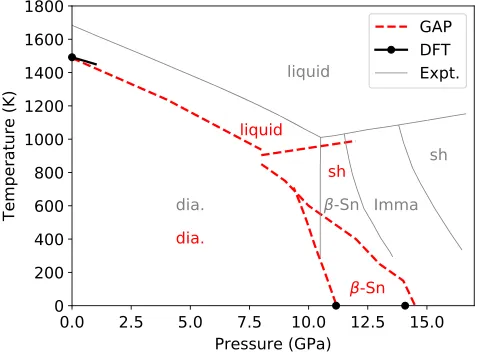
The phase transitions result from a delicate balance between energetic and entropic effects and, for finite-temperature transitions, probe relatively high-energy con-figurations. To calculate the liquid-solid transition lines, we perform coexistence simulations for the diamond and simple hexagonal structure at a fixed pressure and enthalpy and measure the resulting average equilibrium temperature [188]. The diamond-liquid simulations contain 432 atoms, and the pressure is fixed at the values of 0, 4, and 8 GPa; the simple hexagonal-liquid system contains 1024 atoms, and the simulations are carried out at 8 and 12 GPa. To estimate the transition line between β-Sn and simple hexagonal phases, we run isothermic-isobaric molecular-dynamics simulations of both pure phases in a temperature range of 0–1000 K and a pressure range of 6–14 GPa and observe the transition (which occurs in both directions in all cases) by monitoring the Steinhardt bond-order parameters[189]. Finally, the transition line between diamond and β-Sn structures is determined by calculating the Gibbs free energy using the quasiharmonic approximation (QHA). We also establish that in these phases anharmonic con-tributions to the free-energy differences are negligible at 0 K. We use the LAMMPS package for the MD simulations and phonopy[190]for the phonon calculations. Figure10 shows the calculated phase diagram, compared to the published DFT results for the diamond-liquid melting point [191]and our own calculations with the Castep program for the diamond/β-tin and β-tin/simple hexagonal transition pressures at 0 K. For comparison, we also show the experimentally determined phase relations[192]. Note that the Imma phase is missing from the calculated phase diagram, which is due to the fact that both our DFT calculations and GAP model find the Imma phase to be metastable.

E. Defects

1. Point defects

Several point defects are represented in the fitting data-base (TableI), and their formation energies would therefore be expected to be accurately reproduced by the GAP. Indeed, as Fig.1shows, the relative error for the vacancy and three interstitial positions, hexagonal, tetrahedral, and dumbbell, are all within at most 7% of the reference DFT values. The only other potential that is close to this level of accuracy is EDIP, with similar errors for all but the hexagonal interstitial, where it is off by 14%. All the other potentials, as well as DFTB, differ from our DFT calcu-lations by tens of percent for at least some of the defects. Since point defects control properties such as diffusivity in bulk silicon, their migration barriers are also of interest and as they represent bond breaking and formation proc-esses, often present a challenge for interatomic potentials. Since the training database configurations come from finite-temperature MD, it could, in principle, include configurations near the barrier, but, since the system spends relatively little time near the energy saddle point, this is actually unlikely[52]. However, the hexagonal and tetra-hedral interstitials are related by a short displacement, so one is typically a local minimum and the other a saddle point along an interstitial diffusion pathway. We find that the GAP preserves the DFT ordering, although the energy difference is underestimated, while the other potentials make much larger errors, many reversing the relative order of the two high-symmetry geometries. Two other related observables, the migration path of the vacancy and the formation energy of the fourfold defect[193](the midpoint of the concerted-exchange diffusion mechanism[194,195]), which are not represented in the database, are discussed below in Secs.IV EandIV F.

2. Surfaces

Surfaces are a class of defects that have particular importance for the behavior of materials. Solids fail under tension by opening new surfaces, and it is on surfaces that reactions involving chemical species in the environment can take place, where special functional layers can form, e.g., by oxidation, and also where a crystal can grow under suitable conditions. Apart from useful applications, a rich complexity of bonding emerges on surfaces due to the subtle interplay of strain effects with the chemistry of dangling bonds. This complexity makes surface formation energies, and particularly the energies and geometries of various reconstructions, a sensitive test of the accuracy of an interatomic potential.

Figure11shows the energy as a function of separation as a gap is opened up in a unit cell that is long in one direction and has the dimensions of the minimal surface unit cell in the orthogonal plane. For the purposes of this test, the atomic positions are not relaxed but kept rigid relative to FIG. 10. Temperature-pressure phase diagram of silicon,

one another as the gap is opened. All analytical potentials apart from the screened Tersoff show far too short a range—they plateau much earlier than the DFT, and, in fact, this observation is one of the motivating factors behind modifying the original Tersoff potential [131,132]. The right-hand-side limit corresponds to the unrelaxed surface energy in each case, a property in which the potentials show about 30% scatter. Note that, in the case of the (111) surface, the DFT is believed to overestimate the surface energy[196]and, e.g., Tersoff and its screened version are explicitly fit to reproduce the experimental value.

Note that the final version of the fitting database for the GAP presented here includes configurations along the

separation path, in addition to fully separated surfaces. An earlier version of the GAP model[197]that does not include configurations from the separation path correctly reproduces thefully separatedenergy (since fully separated surfaces are included in the fitting) but not the intermediate energies, as shown in the insets in Fig.11. The test results for the version of the potential without the decohesion path configurations (as well as fewer nondiamond crystal structures), listed in detail in Supplemental Material [198], are very close to the final GAP values, with most tested quantities differing by less than 1%. The only exceptions are the quantities directly related to configura-tions newly added to the database and a few other tests (described later in this subsection and in Sec.IV G) that are not explicitly fit [two di-interstitial formation energies that change by 3% and 10% and the (111) reconstructed surface energies that change by 2%–3%]. This example shows that the flexibility of the GAP functional form makes it possible to correct shortcomings by adding configurations to the database without significantly affecting accuracy for other configurations.

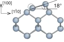
Figure12shows the geometry of the tilted-dimer2×1 reconstruction, one of the low-energy configurations of the (100) surface, which forms spontaneously from the as-cut surface. In this reconstruction, the surface atoms dimerize to form additional bonds, and the dimers tilt (by 18° in our DFT calculations) due to a Jahn-Teller effect[199], which would seem to require an explicit description of the electrons. In fact, none of the analytical potentials repro-duce the substantial tilting (zero tilt for all but EDIP, which tilts by 4°). Only the GAP, with its relatively long-range and flexible form, captures the tilting in reasonable agreement with the DFT (−2.5° error). The DFTB model, with its minimal description of the electronic structure, also shows the breaking of symmetry with a similar error on the resulting bond angle of about−2.3°.

The lowest energy configuration of the (111) surface is the famous 7×7 dimer-adatom-stacking-fault (DAS) recon-struction, already alluded to in the introduction. It is a rather complex structure, involving a 2D superlattice of ten-atom rings, connected by dimerized dislocation cores that separate triangles of stacking faults, half of which have extra atoms on top. A family of analogous structures can be defined by varying the number of dimers,n≥3, between the vertices of FIG. 11. Decohesion energy of diamond-structure silicon along

various directions (labeled according to the orientation of the opening surface). Insets (same axes as the main plot) show errors with respect to the DFT for the current GAP (red) as well as for a previous version of the GAP (gray) with a fitting database that does not include any configurations along the separation path (or high-energy crystal-lattice structures) but only final fully sepa-rated surfaces.

[100]

[110]

-18°

the superlattice, leading to the designation ð2nþ1Þ×

ð2nþ1Þ. As shown in Fig. 13, all analytical potentials predict these reconstructions to be higher in energy than the unreconstructed surface (shown in place of n¼1 for simplicity), and, furthermore, within the family of DAS structures, the energy goes down asngoes up. Computing accurate DFT energies is a nontrivial calculation, and its prediction that the7×7DAS structure is the lowest energy configuration is a significant early triumph of the DFT[113]. Here, our reference is a more recent careful determination of the DFT energies[200]. The DFTB model again stands out as qualitatively different from the analytical models but still fails to show quantitative agreement with the DFT. The GAP model, which includes in its training database just a single configuration of the3×3DAS structure (shown in Fig.14), gives energies with an error below0.05J=m2(much smaller than a meV per atom over the supercell), correctly predicting the DAS family to be lower in energy than the unrecon-structed surface and also giving an energy minimum.

The lowest energy structure for the present potential happens to be for 2nþ1¼5, within 0.01J=m2 of the 7×7 structure. The energy differences are much smaller

than the target (and assumed) error in the GAP model, and as such this level of detail is not robust: The earlier variant of the potential fitted to a slightly different database [in ways unrelated to the (111) surface] show the7×7DAS structure as the global minimum, as shown before[197]. Whatisrobust is the relationship of the energies of the DAS family to other types of reconstructions and the upturn in energy forn¼9. Significantly more data relevant to these structures are needed in order to robustly capture the finest of relative energies within the DAS family.

Figure14shows which atoms are picked (automatically, by the CUR decomposition of the SOAP representation matrix, as mentioned above) to be part of the representative set: mostly those that are unique to the DAS family of reconstruction and do not appear elsewhere in the data set, i.e., the adatom, the atom just below it, one of the dimer atoms in at the boundary of the stacking fault, and one atom on the ten ring that surrounds the vertices of the surface unit cell.

F. Crack propagation

The atomic-scale details of crack propagation prove particularly challenging to model, since sufficient accuracy to describe bond-breaking processes must be combined with large model systems to avoid unrealistic strain gradients [201]. Interatomic potentials which provide an otherwise good description of the bulk and elastic proper-ties of silicon (e.g., the Stillinger-Weber and Tersoff potentials) tend to overestimate the lattice-trapping barriers to brittle fracture, resulting in an overestimate of the fracture toughness as well as an erroneously ductile material response including features such as crack arrest and dislocation emission[116,117,202]. Progress has been made using reactive potentials such as ReaxFF [115] or with hybrid quantum or classical approaches where an ab initio crack-tip model is embedded within a larger classical model system [203–205]. The latter limits the applicability to timescales accessible to the DFT, making it extremely challenging to study processes such as thermally activated crack growth[206].

To test the accuracy of our new GAP model for fracture, we considered the well-studied ð111Þ½1¯10 cleavage system, where fracture is known to exhibit a low-speed instability triggered by the formation of a crack-tip reconstruction [204]. We perform simulations of a 23 496-atom model system of dimensions 600×200×3.86Å3 using both molecular dynamics at 300 K with a range of strain rates between10−6and10−4fs−1and quasistatic strain increments followed by relaxation. In all cases, the trajectories obtained are consistent with those expected from our earlier DFT-based hybrid simulations as reported in Ref.[204]. The GAP model predicts brittle fracture morphology with an atomi-cally smooth fracture surface and the occasional formation of crack-tip reconstruction and subsequent surface steps in the

“downward”½111direction, in line with the results of our FIG. 14. Two views of the DAS 3×3 (111) surface

reconstruction configuration that is in the database with atoms, marked with dark gray, whose environments are selected to be among the representative set for the purposes of defining the GAP model.

previous study. A snapshot from a quasistatic simulation showing the formation of the crack-tip reconstruction at a strain energy release rate of G¼5.13J=m2 is illustrated in Fig.15.

It is worth noting that atoms at the crack tip have rather unique neighbor environments, and, with nothing nearby in the database, the description of crack tips is not reasonable by an earlier version of the potential. But including just a handful (17) of crack tips in the database (using just an

∼200-atom unit cell) already leads to a potential that describes the subtle competition between bond breaking and bond rotation, and qualitatively correct surfaces and crack-tip reconstructions are obtained. The atoms are colored by the predicted error of the GAP model, showing high confidence in the bulk but significant predicted errors at the crack tip, which could be reduced by expanding the database.

IV. RESULTS: VALIDATION

In addition to the tests presented in the previous section, we tested quantities and configurations that are physically important but do not map so cleanly to particular geom-etries in the database. The first is a random structure search, which probes a very wide range of geometries, bonding topologies, and energies. The second is a test of the vibrational properties (harmonic phonons and anharmonic Grüneisen parameters) of the diamond structure, which are only implicitly included in the fit through the perturbed diamond configurations. Finally, two types of defects are

tested, a high-symmetry grain boundary and di-interstitials, which have geometries related to, but clearly different than, the defects in the fitting database.

A. Random structure search

The random structure search (RSS) [207,208] method provides a global test of the potential energy surface, including not only regions near the physically reasonable minima (i.e., typical bulk lattices with small distortions and defects that vary only locally from the bulk structure) but also much more distorted and correspondingly higher energy configurations. We carry out the RSS using the various interatomic potentials and DFT for eight-atom unit cells with constraints on the initial shape (close to cubic) and interatomic distances (>1.7Å) to exclude unphysically close atoms, relaxed with the two-point steepest-descent [209]method. The resulting distribution of configuration energy and volume are plotted in Fig.16. The GAP results show a similar distribution to the DFT, with the diamond structure at the correct volume, a few structures with energies up to 0.2 eV per atom higher, mostly at comparable

FIG. 16. Relaxed volumes and energies (relative to the diamond structure) for random structure search minima. The top left shows a scatter plot with the DFT (black stars), GAP (red stars), and various other interatomic potentials (various color circles). The top right shows the density of states for the minima. The bottom shows a convex hull surrounding all minima for each method with the samexaxis and colors as the top.

50 Å

(a)

(b)

> 0.005 eV

5 Å

< 0.001 eV