Munich Personal RePEc Archive
A Generalized Growth Model and the
Direction of Technological Progress
Li, Defu and Bental, Benjamin
School of Economics and Management, Tongji University,
Department of Economics, University of Haifa
13 October 2019
Online at
https://mpra.ub.uni-muenchen.de/96509/
1
A Generalized Growth Model and the Direction of Technological Progress
Defu Li1
School of Economics and Management, Tongji University Benjamin Bental2
Department of Economics, University of Haifa
Abstract:Based on a general growth model, this paper finds that the steady-state
direction of technological progress is determined by the scale return of the production function and the relative factor supply elasticities. A specific version of that model extends Acemoglu (2002) to provide the underlying determinants of the supply elasticities and demonstrates that the relative price (Hicks, 1932) and relative market size (Acemoglu, 2002) have only a short-term impact on the direction of technological progress. A consequence of the analysis is that the steady-state technological progress is purely labor-augmenting (i.e. delivers Uzawa’s steady-state theorem) if and only if the scale return of the production function is constant and the supply elasticity of capital is infinite. Analogously, an infinite labor supply elasticity is required if labor-augmenting technological progress is to be excluded prior to the Industrial Revolution. Accordingly, changing factor supply elasticities may have induced the Industrial Revolution.
Key Words: Economic Growth, Direction of Technological Progress, Returns to Scale, Factor Supply Elasticities, Uzawa’s Steady-State Theorem, Industrial Revolution
JEL:O33; O41; E13; E25
This Version: October 13, 2019. Comments are welcome!
We are grateful to Oded Galor, Daron Acemoglu, Ryo Horii and Gary H. Jefferson for helpful comments
and suggestions on previous versions of the paper. Li gratefully acknowledges support from the National Natural Science Foundation of China (NSFC:71773083), the National Social Science Foundation of China (NSSFC: 10CJL012). The authors take sole responsibility for their views.
1 School of Economics and Management, Tongji University, 1500 Siping Road, Shanghai, P.R. China,
2 Department of Economics, University of Haifa, 199 Aba Khoushy Ave., Mount Carmel, Haifa, Israel,
2
A Generalized Growth Model and the Direction of Technological Progress
I. Introduction
There is a large and influential body of literature concerning the determinants of the rate of technological progress (see, e.g., Romer, 1990; Aghion and Howitt, 1992). However, the direction of technological progress is not as well understood. In particular, according to Kaldor (1961), post Industrial Revolution economic growth in developed countries has been characterized by increasing per-capita output and physical capital, whereas the capital/output ratio and factor income shares have remained basically constant.3 These facts are generally interpreted as indicating that technological
progress has been purely labor-augmenting. In contrast, Ashraf and Galor (2011) show that during the preindustrial era, technological progress generated population growth and higher density, but not higher per-capita income, which may imply that during that period technological progress lacked labor augmentation. What are the underlying factors implying that labor-augmentation played no role before the industrial revolution but became dominant afterwards? More generally, what determines the direction of technological progress?
Unlike the existing literature (Acemoglu, 2002; Irmen and Tabakovic, 2017), which addresses these questions through the lens of specific growth models, here we first adopt a general approach, assuming a general production function and general factor accumulation processes. Using this setup, we find that, the crucial determinants of the steady-state direction of technological progress are the returns to scale of the production function and the relative factor supply elasticities. In particular, if the production function has constant returns to scale, the steady-state direction of technological progress depends on the relative factor supply elasticities, and is biased towards the factor with the lower elasticity.
A specific version of that model extends Acemoglu’s (2002) micro-mechanism of technological progress to further identify the determinants of the supply elasticities. This version also shows that changing relative factor prices (as suggested by Hicks 1932) and the relative market size (as argued by Acemoglu 2002) do affect the direction of technological progress in the short run, but in steady-state they turn out to have no impact on that direction. The intuition behind this result is the following. In the short run, a higher factor price may encourage not only invention to economize that factor’s use, but also its accumulation. If the supply elasticity of the factor is very large, the
3
invention incentive may be reversed. Furthermore, to offset that factor’s abundance, balanced growth requires an increased investment in technologies that augment the efficiency of the factor with the smaller supply elasticity, which leads to the aforementioned extreme configurations of technological progress.
To fix ideas, consider the case of oil. During a long time period, oil was abundant, and hardly any effort was put into economizing its use, as evidenced by the MPG (Miles per Gallon) figures of cars produced in the U.S. before the 1973 oil crisis.4 That crisis
has caused a sharp increase in oil prices, inducing investment in energy-saving technologies (e.g., increasing MPG). However, the same price increase also induced search for new oil sources, such as shale oil. These new sources have again increased the supply of oil, eventually contributing to sharp price decreases. Consequently, incentives to further invest in energy-saving technologies have decreased.
With this intuition in mind, the paper suggests the following answers to the aforementioned questions. In the pre-industrial era technological progress did not increase labor productivity because labor supply was very elastic (as described by Malthus 1798). Approximately concurrent with the industrial revolution, the demographic transition reduced the supply elasticity of labor. Moreover, the industrial revolution has replaced land by reproducible physical capital. As the supply elasticity of capital increased, there were no incentives to economize on its use and improve its productivity. Consequently, technological progress was biased towards improving human capital, thereby increasing labor productivity. Hence, according to this interpretation, it is the reduction of the labor supply elasticity that has led to the changing direction of technological progress.
Altogether, the contributions of this paper to the literature are as follows: first, within the generalized growth model, it identifies the general factors that determine the direction of technological progress irrespective of the specific parameters of the factor accumulation processes; second, it suggests a specific version of that model with micro-founded technological progress in order to analyze the impact of the production function parameters and those of the factor accumulation processes on the direction of technological progress;third, it delineates the necessary and sufficient conditions that
deliver Uzawa’s (1961) steady-state theorem in the neoclassical growth model; fourth, it highlights the simultaneous impact of the production technology and factor accumulation processes on the direction of technological progress.
The plan of the paper is as follows. Section II discusses the related literature;
4 According to the PEW Environment Group, the model-year 1975 cars drove about 14 miles per gallon. This
4
Section III analyzes the determinants of technological change in a general growth model ; Section IV turns to the same question within a specific model; Section V focuses on some applications: first, Uzawa’s steady-state theorem and second, the Industrial Revolution; SectionVI contains concluding remarks.
II. Related Literature
The direction of technological progress has been a long-standing object of economics research. Hicks (1932) pointed out that changing relative factor prices may affect that direction. Brozen (1953) also pointed out that the direction of technological progress was endogenously determined by economic forces. However, lacking a dynamic growth framework (to be developed by Solow a few years later), these early contributions could not distinguish between short-term and long-term effects.
The neoclassical growth models (Solow, 1956; Swan, 1956) provided this perspective and pointed out that technological progress was the key factor of economic growth in the long run. However, the direction of technological progress turned out to be a cumbersome issue in the neoclassical growth models. As pointed out by Uzawa’s (1961) steady-state theorem, if a neoclassical growth model exhibits steady-state growth, then technological progress must be labor augmenting.5 Although the
steady-state equilibrium with purely labor-augmenting technological progress is consistent with Kaldor’s (1961) stylized facts, there are no compelling intuitive reasons as to why technological progress should per-force take this specific form.
The introduction of an innovation possibility function (Weizsacker, 1962; Kennedy, 1964) coupled with cost reduction maximization, has seemingly enabled the induced innovation literature of the 1960s (Samuelson, 1965; Drandakis and Phelps, 1966) to resolve this issue. However, Nordhaus (1973) questioned the validity of this resolution for its lack of micro-mechanisms generating technological progress. The assumption that enterprises maximize the current rate of cost reduction rather than profits was also criticized (Acemoglu, 2001). In addition, the approach does not clarify the key factors responsible for Uzawa’s theorem.
After nearly 30 years of silence, Acemoglu (1998, 2002, 2003) tried to reactivate the research on the determinants of technological progress based on endogenous growth models (Romer, 1990; Aghion and Howitt, 1992). In these settings, the one-dimensional technology was expanded to two dimensions, enabling researchers and developers to choose between two types of technological innovations. Within this framework,
5
Acemoglu (2002) proposes a market size effect as another key factor affecting the direction of technological progress besides the price effect of Hicks (1932).However, Acemoglu (2002) focuses on the determinants of the steady-state relative level of technology which remains constant only with Hicks-neutral technological progress. When Acemoglu (2003) incorporated the framework into the neoclassical growth model, it again yielded a steady-state growth path with purely labor-augmenting technological progress, failing to explain why enterprises pursuing maximum profits choose only that form of technological progress.
Some additional authors (Funk, 2002; Irmen and Tabakovic, 2017) have constructed growth models which endogenize the direction of technological progress. These models are based on perfect rather than monopolistic competition. However, because the key parameters determining the direction of technological progress are the same as those of the neoclassical growth model, in the steady-state technological progress must still be purely labor-augmenting. Other papers tried to prove that profit-maximizing firms choose to implement purely labor-augmenting technological progress or that the production function converges to the Cobb-Douglas specification (where there is no distinction between various modes of technological progress) based on technology choices among firms (Jones, 2005; Leon-Ledesma and Satchi, 2018). However, these contributions do not discuss what determines the direction of technological progress.
All of the above models share the constraints under which profit-maximizing research and development enterprises choose the direction of technological innovation. Since these constraints are identical to those of the neoclassical growth model, the direction of steady-state technological progress will have to be purely labor-augmenting. Therefore, the direction of technological progress is not determined by whether research and development enterprises can choose technological innovation in different directions, but by the resource endowment conditions that restrict their choices.
steady-6
state is to include also capital-enhancing technological progress. Sato et al. (1999, 2000) also proposed specific models of that nature where steady-states include capital-enhancing technological progress. Irmen (2013) proved that technological progress could include capital-augmentation if adjustment costs become a part of the capital accumulation process. However, these papers do not consider the impact of the production technology on the direction of technological progress. Grossman et al. (2017) introduce an educational input besides capital and labor, and present a growth model that in steady-state admits both capital-enhancing and capital-embodied technological change. Casey and Horii (2019) also build a model with steady-state capital-augmenting technological progress under a linear capital accumulation process by introducing new factors (such as land) into the production function and decreasing returns to scale for capital and labor. It turns out that these papers all circumvent the constraints underlying Uzawa's theorem without explicitly showing what these constraints are to begin with.
In sum, to the best of our knowledge, the existing literature does not consider the simultaneous impact of the production technology and factor accumulation processes on technological progress, and does not provide an overview concerning the determinants of that direction that would be applicable across different models. This is what we do in the remainder.
III.The Determinants of Technological Progress in a General Growth Model
1.Preliminaries
Consider an economy that has two factors of material production, denoted by K and L respectively. What K and L stand for can be determined according to the context of the research questions. For example, K can be capital or land, L can be labor or human capital. For simplicity, we refer to them as “capital” and “labor”. There are two kinds of technologies that can enhance the corresponding material elements, namely a labor-enhancing technology, A, and a capital-enhancing technology, B. The economy has a final output, expressed as Y with a production function given by:
Y(t) = F[B(𝑡)K(𝑡)𝜙, 𝐴(𝑡)L(t)𝜑] ,0 < 𝜙 ≤ 1; 0 < 𝜑 ≤ 1 (1)
Define 𝐾̂(𝑡) ≡ [B(𝑡)K(𝑡)𝜙] as representing effective capital ,and 𝐿̂(t) ≡
[𝐴(𝑡)L(t)𝜑] as representing effective labor. Following Barro and Sala-i-Martin (2004,
7
essential, so that if any of them equals zero, no output is produced.
Define the elasticity of output Y with respect to 𝐾̂(𝑡) and 𝐿̂(t) as 𝛾𝐾̂ ≡𝜕𝐾̂𝜕𝑌𝐾̂𝑌,
𝛾𝐿̂ ≡𝜕𝑌𝜕𝐿̂𝑌𝐿̂. Because the production function has constant return to scale, 𝛾𝐾̂+ 𝛾𝐿̂ = 1.
The output elasticity with respect to K and L is defined as 𝛽K≡ 𝜕𝑌𝜕𝐾K𝑌 , 𝛽L≡𝜕𝑌𝜕L𝑌L,
implying 𝛽K = 𝜙𝛾𝐾̂ , 𝛽L= 𝜑𝛾𝐿̂ . When 𝜙 = 𝜑 = 1 , then 𝛽K+ 𝛽L = 𝛾𝐾̂+ 𝛾𝐿̂ = 1 ,
and the function F(·) exhibits constant returns to scale with respect to K and L;when 𝜙 < 1; 𝜑 = 1 , or 𝜙 = 1; 𝜑 < 1 , then 𝛽K+ 𝛽L< 1,and the function F(·) exhibits
diminishing returns to scale with respect to K and L. Therefore, 𝜙 and 𝜑 are the
return to scale factors with respect to K and L, respectively.
Output per effective labor is expressed by 𝑦(t) ≡Y(t)𝐿̂(t)= 𝐴(𝑡)L(t)Y(t) 𝜑 and effective
capital per effective labor is expressed by 𝑘(t) ≡𝐾̂(𝑡)𝐿̂(t) =B(𝑡)K(𝑡)𝐴(𝑡)L(t)𝜑𝜙 . Accordingly, the production function in the intensive form becomes:
y(t) = F [B(𝑡)K(𝑡)𝐴(𝑡)L(t)𝜑𝜙, 1] = 𝑓(𝑘(𝑡)) (2)
Factor prices are assumed to equal the respective marginal products of K and L, i.e.:
{𝑤(𝑡) = 𝜑𝐴(𝑡)𝐿(𝑡)𝜑−1[𝑓(𝑘) − 𝑘𝑓′(𝑘)]
r(t) = 𝜙𝐵(𝑡)𝐾(𝑡)𝜙−1𝑓′(𝑘) (3)
Equations (3) show that the return to scale factors 𝜑 and 𝜙 have important influence on factor prices. When they are less than 1, even if 𝑘 is constant, a factor’s price decreases with the increase of its quantity.6
In the general model, the factor supply functions are not specified, but are assumed to depend on the respective factor prices. The price elasticities are the key characteristic of the respective factor supplies, and are given by:
{
𝜀𝐾 ≡K̇(t)/𝐾(𝑡)𝑟̇(t)/𝑟(𝑡)
𝜀𝐿 ≡ 𝑤̇(t)/𝑤(𝑡)L̇(t)/𝐿(𝑡)
(4)
2. The Direction of Technological Progress: Definition
6
8
The direction of technological progress, DTP, is the ratio between the rates of capital- and labor-augmenting factors, i.e.
𝐷𝑇𝑃 ≡ Ḃ(t)/B(t)
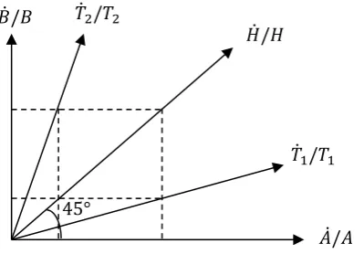
Ȧ(t)/𝐴(𝑡) (5) The range of DTP is [0, ∞]. When 𝐵̇/𝐵 = 0 and 𝐴̇/𝐴 > 0 then 𝐷𝑇𝑃 = 0, and technological progress is purely labor-augmenting (i.e. Harrod-neutral); when 𝐵̇/𝐵 > 0 and 𝐴̇/𝐴 = 0 then 𝐷𝑇𝑃 → +∞ , and technological progress is purely capital-augmenting (i.e. Solow-neutral); when 𝐵̇/𝐵 = 𝐴̇/𝐴 > 0 then 𝐷𝑇𝑃 = 1 , and technological progress is Hicks-neutral. Figure 1 shows different directions of technological progress.
Clearly, the axes represent Harrod-neutral (horizontal) and Solow-neutral (vertical) technological changes. The diagonal 𝐻̇/𝐻 represents the location of Hicks-neutral technological changes. The ray 𝑇̇1/𝑇1 indicates technological progress which tends to
be more labor augmenting, while 𝑇̇2/𝑇2 is more capital augmenting.
Note, that the direction of technological progress is related to the direction of technology (DT), given by 𝐷𝑇 ≡ B(t)/𝐴(𝑡). Obviously, the direction of technological progress determines the direction of technology, but they are fundamentally different. Specifically, when the direction of technological progress is Hicks neutral, the direction of technology remains unchanged. Otherwise the direction of technology will continuously rise or fall.
3.The Determinants of DTP: General Statement
[image:9.595.207.407.308.447.2]Along a steady-state path the growth rates of Y(t), B(𝑡), K(𝑡), 𝐴(𝑡) and L(t) are constant. Furthermore, 𝑘(t) ≡B(𝑡)K(𝑡)𝐴(𝑡)L(t)𝜑𝜙 is also constant, implying:
Figure 1: Direction of technological progress
𝑇̇1/𝑇1 𝐻̇/𝐻 𝑇̇2/𝑇2
𝐵̇/𝐵 Ḃ/
𝐴̇/𝐴 5°
9
𝜙K̇(t) K(t) +
Ḃ(t) B(t) = 𝜑
L̇(t) L(t) +
Ȧ(t)
A(t) (6) In Appendix A we prove the following proposition.
Proposition 1:If the production function of an economy satisfies equation (1) and factor prices equal their respective marginal products, then the steady-state direction of technological progress is given by:
𝐷𝑇𝑃 = (1 + 𝜀𝐿)/[1 + (1 − 𝜑)𝜀𝐿]
(1 + 𝜀𝐾)/[1 + (1 − 𝜙)𝜀𝐾] (7)
According to proposition 1, there are two factors that determine the steady-state direction of technological progress: one is the price elasticities of the factor supplies, 𝜀𝐿 and 𝜀𝐾; the other is the factors’ return to scale parameters, 𝜙 and 𝜑. The former
reflects the factor accumulation processes, while the latter reflects the production function. Given 𝜙 and 𝜑, technological progress tends to the factor with the smaller supply elasticity, while it tends to the factor with the smaller return to scale when the factor supply elasticities are given. The relative price (Hicks, 1932) and relative market size (Acemoglu, 2002) do not affect the steady-state direction of technological progress.
For the constant returns to scale (CRS) neoclassical growth model, i.e. 𝜙 = 𝜑 = 1, we obtain:
Corollary 1: in the CRS casethe direction of technological progress is determined by:
𝐷𝑇𝑃 =1 + 𝜀1 + 𝜀𝐿
𝐾 (8)
Corollary 1 shows that for the CRS case the steady-state direction of technological progress is determined solely by the relative primary factor supply elasticities and is biased towards the one with the relatively smaller elasticity.
10
IV.The Determinants of DTP in a Specific Growth Model
The Acemoglu (2002) growth model expanded the Romer (1990) technology from one dimension to two. However, it provided only the determinants of the direction of
technology rather than that of technological progress, and that only when the steady-state technological progress is Hicks neutral. The current paper extends the Acemoglu model in two aspects: one is to allow the production function to admit diminishing returns to scale; the other is to expand the investment elasticities of the factor accumulation processes allowing also the presence of capital-embodied technological progress.
1. The model
We briefly reiterate the Acemoglu (2002) model and emphasize our extensions. The economy consists of two kinds of material factors, and three sectors of production; a final goods sector, an intermediate goods sector and a research and development (R&D) sector. The symbols K, L, S represent two kinds of material production factors and “scientists” who specialize in the research and development of new intermediate products, respectively.
The household’s goal is to maximize the discounted flow of utility, given by:
U = ∫∞𝐶(𝑡)1 − 𝜃1−𝜃− 1𝑒−𝜌𝑡𝑑𝑡
0 (9)
where 𝐶(𝑡) is consumption at time t, ρ>0 is the discount rate, and θ>0 is a utility curvature coefficient of the household.
The household’s periodic budget constraint is given by:
𝐶 + 𝐼𝐾+ 𝐼𝐿 = 𝑌 = 𝑤𝐿 + 𝑟𝐾 + w𝑆𝑆 (10)
where the LHS stands for expenditures consisting of consumption and investments 𝐼𝐾
and 𝐼𝐿 into capital and labor, and the RHS is income, obtained from renting out labor
at the rate w, capital at the rate r and scientists at the rate w𝑆.
The final goods sector is competitive, using the following production functions:
𝑌 = [𝛾𝑌𝐿(𝜀−1)/𝜀+ (1 − 𝛾)𝑌𝐾(𝜀−1)/𝜀]𝜀/(𝜀−1), 0 ≤ 𝜀 < ∞ (11)
where Y is output and YL and YK are the two inputs, with the factor-elasticity of
substitution given by ε.
11
substitution (CES) production functions using a continuum of intermediate inputs, 𝑋(𝑖) and 𝑍(𝑗):
𝑌𝐿 = [∫ 𝑋(𝑖)𝜑𝛽𝑑𝑖 𝑁
0 ]
1/𝛽
𝑎𝑛𝑑 𝑌𝐾 = [∫ 𝑍(𝑗)𝜙𝛽𝑑𝑗 𝑀
0 ]
1/𝛽
(12)
where the elasticity of substitution is given by 𝑣 = 1/(1– 𝛽) and N and M represent the measure of the two types of the intermediate inputs, respectively. The specification of the production functions extends that of Acemoglu’s by introducing the parameters 𝜑 and 𝜙 and assuming that 0 < 𝜑 ≤ 1 , 0 < 𝜙 ≤ 1 . When𝜑 = 𝜙 = 1 , equations (12) degenerate to the form used in Acemoglu (2002). When 𝜑 < 1 or 𝜙 < 1, then production of the inputs is characterized by diminishing returns to scale.
The intermediate factors 𝑋(𝑖) are produced by labor, whereas 𝑍(𝑗) are produced by capital, where the respective production functions are linear:
𝑋(𝑖) = 𝐿(𝑖) and 𝑍(𝑗) = 𝐾(𝑗) (13) Accordingly, 𝑌𝐿 and 𝑌𝐾 represent labor-intensive and capital-intensive inputs
respectively. New intermediate inputs are developed by an R&D department. The innovation functions are specified as follows7
{𝑁̇ = 𝑑𝑁𝑁𝑆𝑁− 𝛿𝑁
𝑀̇ = 𝑑𝑀𝑀𝑆𝑀− 𝛿𝑀 (14)
where 𝑆𝑁 and 𝑆𝑀 represent respectively the number of scientists engaged in
innovation of the two kinds of intermediate inputs. The total number of scientists is exogenously set at S, so 𝑆𝑁+ 𝑆𝑀 ≤ 𝑆. Once a new intermediate input is invented, the
inventor obtains a permanent patent, as in Romer's (1990) model.
Another important extension of Acemoglu (2002) in this paper is the following specification of the factor accumulation processes:
{𝐾̇ = 𝑞(𝑡)𝐼𝐾
𝛼𝐾 − 𝛿
𝐾𝐾, 𝑞̇(𝑡)/𝑞(𝑡) = 𝑔𝑞≥ 0,0 ≤ 𝛼𝐾 ≤ 1, 𝛿𝐾 > 0
𝐿̇ = 𝑏𝐿𝐼𝐿𝛼𝐿− 𝛿𝐿𝐿,𝑏𝐿 > 0,0 ≤ 𝛼𝐿 ≤ 1 , 𝛿𝐿 > 0
(15)
There are two key differences between equations (15) and the analogous Acemoglu specification: the introduction of investment elasticity parameters 𝛼𝐾 and 𝛼𝐿 and the
7 The experimental equipment model (Rivera-Natiz and Romer, 1991) can also be used to construct the
12
inclusion of possible capital-embodied technological progress at the exogenously given rate 𝑞̇(𝑡)/𝑞(𝑡) = 𝑔𝑞.
Two comments are in order concerning these extensions. First, while it may be difficult to empirically estimate 𝛼𝐾 and 𝛼𝐿 , various models have taken a stand on
their values. For example, the “standard” neoclassical growth model implicitly sets 𝛼𝐾 11,8 . whereas the Malthusian model implicitly sets 𝛼𝐿 11.9 Acemoglu’s (2002)
assumption that K and L are exogenously given amounts to setting 𝛼𝐾 and 𝛼𝐿 to
zero.10 Irmen (2013) points out theoretically that 𝛼
𝐾<1 may be more reasonable to
account for adjustment costs of material capital investment. To capture such possibilities, we assume their values to range from 0 to 1.
Second, the introduction of potential capital embodied technological progress is aimed at accommodating the observed declining trend of the relative price of capital goods (see, e.g., Grossman et al. 2017).
2. The market equilibrium
Given the setting of the model, the final goods sector and intermediate goods sector will be in equilibrium when both the final goods firms and the intermediate goods firms maximize their profits and the markets of capital and labor clear. Given the goods market equilibrium, the following two propositions hold:
Proposition 2: In the market equilibrium, the final output production function takes the form:
𝑌 = [𝛾(𝐴𝐿𝜑)(𝜀−1)/𝜀+ (1 − 𝛾)(𝐵𝐾𝜙)(𝜀−1)/𝜀]𝜀/(𝜀−1) (16)
where 𝐴 ≡ 𝑁(1−𝜑𝛽)/𝛽and 𝐵 ≡ 𝑀(1−𝜙𝛽)/𝛽.
Proof:See Appendix B.
The CES equation (16) is a specific form of the production function (1), with
8 Under the commonly used assumption of an exogenously growing labor force, 𝛼
𝐿 is not specified.
9 If we let 𝐼
𝐿≡ 𝑠𝐿𝑌,then 𝐿̇ = 𝑏𝐿𝐼𝐿− 𝛿𝐿𝐿 = 𝑠𝐿𝑏𝐿𝑌 − 𝛿𝐿𝐿 . This is the labor supply hypothesis of the
Malthusian model, where 𝑠𝐿 is endogenously determined by the family's intertemporal optimization.
10 Note that when the embodied technological progress is not taken into account, q(t) is a constant. Therefore,
at the steady-state values of 𝐾̇ = 0 and 𝐿̇ = 0 we obtain 𝐾∗= 𝑞̅/𝛿
13
constant returns to scale to 𝐴𝐿𝜑 and 𝐵𝐾𝜙. With respect to 𝐿 and 𝐾, it has constant
returns to scale when 𝜑 = 1 and 𝜙 = 1 and diminishing returns to scale when 𝜑 < 1 or 𝜙 < 1.
Proposition 3:In the goods market equilibrium, the relative benefits of
innovation of capital-intensive and labor-intensive intermediate goods are determined by:
𝜋𝑀
𝜋𝑁 =
(1 − 𝜙𝛽)𝜑 (1 − 𝜑𝛽)𝜙 .
𝑟 𝑤 .
𝐾 𝐿 .
𝑁
𝑀 (17) where 𝜋𝑀 and 𝜋𝑁 represent the monopoly profits of capital-intensive and
labor-intensive intermediate goods producers. Proof:See Appendix C.
Equation (17) shows that for a given ratio of the technology levels, represented here by M/N, relative invention profits are positively related to the relative factor prices (r/w) and the relative factor supplies (K/L). Accordingly, a change of the relative price encourages innovations directed at the scarce factor whose price has increased, as suggested by Hicks (1932). Acemoglu (2002) noted that the relative amount of the two factors, (K/L), has two countervailing effects on 𝜋𝑀/𝜋𝑁. On the one hand, a higher K/L
causes an increase in 𝜋𝑀/𝜋𝑁, which in turn leads to a technological change favoring
the abundant factor (“the market size effect”). On the other hand, a higher K/L decreases 𝑟/𝑤 and 𝜋𝑀/𝜋𝑁, which is the price effect of a change in K/L. The total effect of a
change in K/L is regulated by the elasticity of substitution 𝜀 between the two factors. If 𝜀 > 1 , the market size effect dominates the price effect, and increasing K/L will encourage favoring improvements of the abundant factor. Otherwise, when 𝜀 < 1 , improvements of the scarce factor will be favored.
14
intermediate factor causes M/N to increase. Equation (17) then shows that a higher M/N
implies an decrease in 𝜋𝑀/𝜋𝑁, discouraging further inverstment into innovations in
the capital-intensive sector. Moreover, equation (17) represents only the demand side of technological change. To get the long-run effects, it is necessary to consider also factors affecting the supply of innovations and material factors, in particular that of 𝑟/𝑤 on K/L and of 𝜋𝑀/𝜋𝑁 on 𝑀/𝑁 , within a dynamic general equilibrium
framework. As will be shown below, in such a context, even if there is a short-run “market size effect”, K/L and M/N cannot be both continually increasing in the long-run.
3.The Steady State
When the goods market and the scientist market are in equilibrium and households maximize their utility, the economy arrives at a steady-state growth equilibrium in which each endogenous variable grows at a constant rate. The following proposition shows that the model has a unique steady-state growth equilibrium.
Proposition 4: there exists a unique steady-state growth equilibrium in which the resource allocation is determined by equations (18), and the steady-state growth rates are determined by equations (19).
{
𝑆𝑁∗ =𝜒2(𝑑𝑀𝑆 − 𝛿) + 𝜒𝜒 1𝛿 + 𝛽(1 − 𝜑𝛼𝐿)𝜙𝑔𝑞 1𝑑𝑁+ 𝜒2𝑑𝑀
𝑆𝑀∗ =𝜒1(𝑑𝑁𝑆 − 𝛿) + 𝜒𝜒 2𝛿 − 𝛽(1 − 𝜑𝛼𝐿)𝜙𝑔𝑞 1𝑑𝑁+ 𝜒2𝑑𝑀
𝑠𝐿∗ = (𝛼𝐿𝑔 + δL)𝛼𝐿𝛽𝜑 2
𝜌 + δL− (1 − 𝛼𝐿− 𝜃)𝑔 .
𝜒4𝑑𝑀
𝜒3𝑑𝑁+ 𝜒4𝑑𝑀
𝑠𝐾∗ = (𝛼𝐾g + δK)𝛼𝐾𝛽𝜙 2
𝜌 + δK− (1 − 𝛼𝐾− 𝜃)g .
𝜒3𝑑𝑁
𝜒3𝑑𝑁+ 𝜒4𝑑𝑀
𝑠𝐶∗ = 1 − 𝑠𝐾∗− 𝑠𝐿∗
15
{
(𝑌𝑌)̇ ∗= (𝐼̇𝐼𝐿
𝐿) ∗
= (𝐼̇𝐼𝐾
𝐾) ∗
= (𝐶𝐶̇)
∗
= 𝑔
(𝐾̇ 𝐾)
∗
= α𝐾𝑔 + 𝑔𝑞
(𝐿̇𝐿)
∗
= 𝛼𝐿𝑔
(𝑀̇𝑀)
∗
=1 − 𝜙𝛽 [𝛽 (1 − 𝜙𝛼𝐾)g − 𝜙𝑔𝑞]
(𝑁̇𝑁)
∗
= 1 − 𝜑𝛽𝛽 (1 − 𝜑𝛼𝐿)𝑔
𝑔 ≡(1 − 𝜑𝛽)𝛽 (1 − 𝜙𝛽)[𝑑𝑀dN𝜒𝑆 − (dN+ 𝑑𝑀)δ] + 𝜙𝛽dN𝑔𝑞
1𝑑𝑁+ 𝜒2𝑑𝑀
(19)
where 𝜒1 ≡ (1 − 𝜑𝛽)(1 − 𝜙𝛼𝐾) , 𝜒2 ≡ (1 − 𝜙𝛽)(1 − 𝜑𝛼𝐿) , 𝜒3 ≡ (𝜑 − 𝜑2𝛽)
and 𝜒4 ≡ (𝜙 − 𝜙2𝛽).
Proof: See Appendix D.
Equations (18) define the household resource allocations, i.e. that of scientists into the two kinds of innovations 𝑆𝑁∗ and 𝑆𝑀∗ , and that of income into the
accumulation processes and consumption, implying two saving rates 𝑠𝐾 ≡ 𝐼𝐾/𝑌, 𝑠𝐿 ≡
𝐼𝐿/𝑌 and a consumption rate 𝑠𝐶 ≡ 𝐶/𝑌. Equations (19) deliver the steady-state growth
path at the resource allocation given by equations (18).
While Proposition 1 assumes that the general growth model steady-state equilibrium exists, equations (18) and (19) show that in the specific growth model it is in fact the case. Moreover, the steady-state equilibrium is unique.
Proposition 5:In the specific growth model, the factor supply elasticities are
determined by equation (20) as follows:
{
𝜀𝐾 = (1 − 𝛼α𝐾 + 𝑔𝑞/𝑔 𝐾) − 𝑔𝑞/𝑔
𝜀𝐿 =1 − 𝛼𝛼𝐿
𝐿
(20)
Proof: See Appendix E.
16
process, 𝛼𝐾 and 𝛼𝐿, determine the factor supply elasticities, 𝜀𝐾 and 𝜀𝐿. When 0 ≤
𝛼𝐾 ≤ 1 − 𝑔𝑞/𝑔, then 0 ≤ 𝜀𝐾 ≤∞, and 0 ≤ 𝜀𝐿 ≤∞ when 0 ≤ 𝛼𝐿 ≤ 1.11
Substituting equations (20) into equation (7), we obtain
𝐷𝑇𝑃 = (1 + 𝜀(1 + 𝜀𝐿)/[1 + (1 − 𝜑)𝜀𝐿]
𝐾)/[1 + (1 − 𝜙)𝜀𝐾] =
(1 − 𝜙𝛼𝐾) − 𝜙𝑔𝑞/𝑔
(1 − 𝜑𝛼𝐿) (21)
Since 𝐴 ≡ 𝑁(1−𝜑𝛽)/𝛽and 𝐵 ≡ 𝑀(1−𝜙𝛽)/𝛽, from equation (19) we then get:
{(𝐵̇/𝐵)∗ = (1 − 𝜙𝛼𝐾)𝑔 − 𝜙𝑔𝑞 (𝐴̇/𝐴)∗ = (1 − 𝜑𝛼
𝐿)𝑔 (22)
Equation (21) can be also obtained by substituting equations (22) into equation (5) which is the definition of DTP. The resulting equation not only confirms proposition 1, but also gives the concrete determinants of the steady-state direction of technological progress in the specific model.
V.Applications
I:Uzawa’s Steady-State Theorem
Uzawa's (1961) steady-state theorem challenges growth theory. It holds that in steady-state, technological progress in the neoclassical growth model cannot include capital-augmentation. However, the theorem does not reveal the underlying factors that are responsible for the conclusion. Based on the results of the general and specific models above, it becomes possible to provide the necessary and sufficient conditions required to obtain Uzawa’s theorem. As a consequence, the exact conditions under which the steady-state of a growth model can admit capital-augmenting technological are revealed.
1.Necessary and Sufficient Conditions for Uzawa’s Steady-State Theorem
By proposition 1, the following corollary, proven in Appendix F, holds:
Corollary 2 (Uzawa’s Steady-State Theorem): Suppose the production function of a growth model is characterized by equation (1). Then, along the steady-state equilibrium path technological progress cannot include capital-augmentation
(i. e.Ḃ(t)B(t)= 0) if and only if capital has an infinite supply elasticity (i. e. 𝜀𝐾 = ∞) and
the capital return to scale is constant (i. e. 𝜙 = 1).
11 It is worth noting that if 𝛼
𝐾> 1 − 𝑔𝑞/𝑔 then 𝜀𝐾< 0, which means that the factor supply is negatively
17
2. Discussion of Corollary 2
First, the traditional neoclassical growth model satisfies the necessary and sufficient conditions of Uzawa's steady-state theorem. In these models the production function is specified as Y(t) = F[B(𝑡)K(𝑡), 𝐴(𝑡)L(t)] , with a capital accumulation process 𝐾̇ = 𝐼 − 𝛿𝐾. Furthermore, there is no capital-embodied technological progress. This specification implies 𝜙 = 1, 𝛼𝐾 = 1, 𝑔𝑞 = 0. According to equations (20), this
implies 𝜀𝐾 = ∞. Therefore, the traditional neoclassical growth model cannot include
capital-augmenting technological progress in steady-state.
Second, while the existing literature has discussed the conditions of Uzawa's steady-state theorem, it has not clearly and completely pointed out the necessary and sufficient conditions underlying its validity.
For example, Acemoglu (2003) and Jones and Scrimgeour (2008) argue that the asymmetry between capital and labor growth processes (endogenous growth of capital and exogenous growth of labor) are the key to explain the theorem, but corollary 2 shows that whether capital-augmenting technological progress may be part of a steady-state equilibrium has nothing to do with labor growth.
Sato (1996) pointed out that the linear specification of the capital accumulation process, that is, 𝛼𝐾 = 1, is necessary for the steady state to exclude capital-augmenting
technological progress. However, according to Corollary 2,on the one hand, if 𝜙 = 1, the specific growth model of Section IV also excludes capital-augmentation even though 𝛼𝐾 = 1 −𝑔𝑔𝑞 < 1 ; on the other hand, even though 𝛼𝐾 = 1 and 𝜀𝐾 = ∞ ,
technological progress will include capital-augmentation in steady state, provided that 𝜙 < 1 and 𝑔𝑞 = 0,.
Grossman et al. (2017) specified the production function as Y = F[BK, 𝐴L, 𝑠] , where s stands for schooling, alongside a capital accumulation process 𝐾̇ = 𝑞(𝑡)𝐼 − 𝛿𝐾. They argue that 𝑠̇ = 0 is the necessary condition for the steady-state to exclude capital-augmenting technological progress. But again, on the one hand, as they point out by themselves, if there exists a measure of human capital, H(AL,s), such that 𝐹(𝐵𝐾, 𝐴𝐿, 𝑠) ≡ F̃[BK, H(𝐴L, 𝑠)] , then even if 𝑠̇ > 0 , the steady-state cannot admit capital-augmenting technological change; on the other hand, by Corollary 2, if 𝜙 < 1 or 𝛼𝐾 < 1, the specific growth model of Section IV will include capital-augmentation
18
Third, as long as any condition of Corollary 2 is not satisfied, technological progress does include capital-augmentation in steady state.
(1) 𝝓 = 𝟏, 𝜺𝑲< ∞.
Under these conditions, whatever 𝜀𝐿 and 𝜑 may be, Proposition 1 implies
𝐷𝑇𝑃 =(1+𝜀𝐿)/[1+(1−𝜑)𝜀𝐿]
1+𝜀𝐾 > 0, i.e.
Ḃ(t)
B(t)> 0. In the specific model of Section IV, as long
as 0 < 𝛼𝐾 < 1 − 𝑔𝑞/𝑔, setting 𝜙 = 1 implies 0 < 𝜀𝐾 < ∞ by equation (20). As a
result, from equation (22), Ḃ(t)B(t)= (1 − 𝛼𝐾)𝑔 − 𝑔𝑞> 0. Especially, for 𝑔𝑞 = 0, 0 <
𝛼𝐾 < 1 is necessary to obtain 0 < 𝜀𝐾 < ∞. Sato (1999, 2000) and Irmen (2013) fit
into this parameter configuration. (2) 𝜺𝑲= ∞, 𝝓 < 𝟏.
Here, as long as 𝜀𝐿 and 𝜑 are within their admissible domains, Proposition 1
implies 𝐷𝑇𝑃 = (1+𝜀𝐿)/[1+(1−𝜑)𝜀𝐿]
(1+𝜀𝐾)/[1+(1−𝜙)𝜀𝐾]> 0 and
Ḃ(t)
B(t)> 0. In the model of Section IV with
𝛼𝐾 = 1 − 𝑔𝑞/𝑔 , equation (20) yields 𝜀𝐾 = ∞ . But then, with 𝜙 < 1 equation (22)
implies 𝐵̇/𝐵 = (1 − 𝜙)𝑔 > 0.
The effect of the return to scale on the steady-state direction of technological progress has been neglected in the existing literatures. Recently, Casey and Horii (2019) actually rendered 𝜙 < 1 by considering land as an input. Therefore, in their case capital augmentation is part of the steady-state equilibrium. Specifically, because they assume 𝛼𝐾 = 1 and 𝑔𝑞 = 0 , K̇(t)K(t)= Ẏ(t)Y(t) and the ratio of capital to output (K/Y)
remains unchanged.
(3) Reconciling 𝒈𝒒 > 𝟎 with 𝑩̇𝑩> 𝟎.
Grossman et al. (2017) argue that the United States is on a balanced growth path with falling investment-good prices and that the elasticity of substitution between capital and labor is less than unitary. In their view, growth models should generate steady-states with capital-embodied as well as capital-augmenting technological progress. As mentioned above, they introduce a schooling variable into the production function in order to achieve this goal. However, according to Corollary 2 the same desiderata are obtained without the introduction of an additional factor if 𝜀𝐾 < ∞ or
𝜙 < 1 . For example, according to equation (22), as long as (1−𝜙𝛼𝐾)
𝜙 >
𝑔𝑞
𝑔 , then the
19
path.12
II:Industrial Revolution
As mentioned above, according to Ashraf and Galor's (2011) empirical work and Kaldor's (1961) styled facts, before the Industrial Revolution technological progress was almost purely land-augmenting, excluding labor-augmentation, and after the Industrial Revolution technological progress was basically labor-augmenting, excluding capital-augmentation. In terms of the above analysis, what are the underlying factors that cause such tremendous differences in the direction of technological progress?
Suppose the production function is characterized by constant returns to scale (𝜙 = 𝜑 = 1) and no capital-embodied technological progress (𝑔𝑞 = 0). If 𝛼𝐿 = 1 and 𝛼K <
1, equation (22) implies 𝐴̇𝐴= 0,𝐵̇
𝐵> 0, and equation (19) implies 𝑌̇
𝑌−
𝐿̇
𝐿 =
𝐴̇ 𝐴 = 0,
𝑌̇
𝑌−
𝐾̇
𝐾 =
𝐵̇
𝐵> 0 . Interpreting K as “land”, this is consistent with Ashraf and Galor's (2011)
empirical study of the pre-Industrial Revolution era. Under the above conditions, equation (20) implies an infinite labor supply elasticity (𝜀𝐿 = ∞ ) and a finite land
supply elasticity (𝜀𝐾 < ∞). These generate a long-term stagnation of per capita income,
consistent with the situation before the Industrial Revolution. In other words, the abundance of labor caused technological progress to be purely land-augmenting, leading to the Malthusian subsistence-level trap.
Similarly, if 𝛼K= 1 (i.e. capital becomes abundant) and 𝛼𝐿 < 1 , the rate of
capital-augmenting technological progress is zero and the rate of labor-augmenting technological progress is greater than zero, that is, 𝐵̇𝐵= 0 and 𝐴̇𝐴 > 0. From equations
(19), the growth rate of capital is the same as that of output (𝑌̇𝑌= 𝐾̇𝐾), keeping the ratio
of capital to output (K/Y) unchanged. Moreover, per capita income is increasing (𝑌̇𝑌−
𝐿̇
𝐿=
𝐴̇
𝐴> 0). This is consistent with Kaldor’s styled facts concerning the era after the
Industrial Revolution. The above analysis then implies that the change of the labor supply elasticity from infinite to finite, and that of material elements from a finite supply elasticity of land to an infinite supply elasticity of capital may hold the key to the emergence of the Industrial Revolution.
How these supply elasticities might have changed is not yet fully explained. The
12 In fact, Grossman et al. (2017) also get their results by 𝜀
𝐾< ∞. However, their capital supply elasticity
20
Unified growth theory of Galor (2011) suggests an endogenous transformation mechanism whereby the labor supply elasticity changes from infinite to zero. Therefore, it can explain how technological progress has changed from one that excludes steady-state labor augmentation to one that includes it. Because the theory focuses on the transition from stagnant to continually growing per capita income, it does not consider the change of the supply elasticities of land and capital. As a result, it has not yet explained why technological progress became purely labor augmenting after the Industrial Revolution, as is required to meet Kaldor's styled facts.
VI Concluding Remarks
Using a generalized growth model, this paper proves that the determinants of the direction of technological progress in a steady-state equilibrium depends on two aspects: the relative size of returns to scale of different inputs in the production function and the relative size of the supply elasticities of these inputs. A specific version that extends the Acemoglu (2002) model provides micro-foundation for technological progress and explicit formulation of the underlying factors affecting the direction of technological progress. Both the general model and the specific one show that although the relative price (Hicks, 1932) and the relative market size (Acemoglu, 2002) affect the short-term direction of technological progress, they have no impact on that direction in steady-state.
21
22
Appendix A:The derivation process of equation (7)
Dividing the denominator of equation (5) by the two sides of equation (6) yields:
𝐷𝑇𝑃 = Ḃ(t)/B(t) Ȧ(t)/𝐴(𝑡)=
Ḃ(t)
B(t) / [Ḃ(t)B(t) + 𝜙K̇(t)K(t)] Ȧ(t)
𝐴(𝑡) / [𝐴(𝑡) + 𝜑Ȧ(t) 𝐿(𝑡)]L̇(t)
= 1 + 𝜑 L ̇(t) 𝐿(𝑡) /𝐴(𝑡)Ȧ(t)
1 + 𝜙 KK(t) /̇ (t) Ḃ(t)B(t) (A1) The growth rates of 𝑟(𝑡) and 𝑤(𝑡) in equations (3) are obtained by taking 𝑘(𝑡) as a constant, yielding:
{ 𝑤̇(t)
𝑤(𝑡) = Ȧ(t)
𝐴(𝑡) + (𝜑 − 1) L̇(t) 𝐿(𝑡) 𝑟̇(t)
𝑟(𝑡) = Ḃ(t)
B(t) + (𝜙 − 1) K̇(t) K(t)
(𝐴2)
Substituting equations (A2) into equations (4) then yields:
{
𝜀𝐿 = Ȧ(t) L̇(t)/𝐿(𝑡)
𝐴(𝑡) + (𝜑 − 1)L̇(t)𝐿(𝑡) 𝜀𝐾 = Ḃ(t)K̇(t)/𝐾(𝑡)
B(t) + (𝜙 − 1)𝐾(𝑡)K̇(t)
(𝐴3)
From equations (A3) we obtain:
{ L̇(t) 𝐿(𝑡) / Ȧ(t) 𝐴(𝑡) = 𝜀𝐿
1 + (1 − 𝜑)𝜀𝐿
K̇(t) K(t) /
Ḃ(t) B(t) =
𝜀𝐾
1 + (1 − 𝜙)𝜀𝐾
(𝐴4)
Substituting equations (A4) into equation (A1) and rearranging implies equation (7):
𝐷𝑇𝑃 =(1 + 𝜀(1 + 𝜀𝐿)/[1 + (1 − 𝜑)𝜀𝐿]
𝐾)/[1 + (1 − 𝜙)𝜀𝐾]
Appendix B: Proof of Proposition 2.
Letting the final good serve as numeraire, the representative competitive final good producer faces the input prices 𝑝L and 𝑝K and selects the respective 𝑌𝐾 and 𝑌𝐿
so as to maximize
𝜋𝑌 = 𝑌 − 𝑝L𝑌𝐿− 𝑝K𝑌𝐾 (𝐵1)
23
{𝑝𝐾 = (1 − 𝛾)[𝛾 + (1 − 𝛾)(𝑌𝐾/𝑌𝐿)(𝜀−1)/𝜀]1/(𝜀−1)(𝑌𝐾/𝑌𝐿)−1/𝜀
𝑝𝐿 = 𝛾[𝛾 + (1 − 𝛾)(𝑌𝐾/𝑌𝐿)(𝜀−1)/𝜀]1/(𝜀−1) . (𝐵2)
The reperesentative producers of YK and YL maximize their profits by choosing
Z(j) and X(i), given the intermediate input prices 𝑝Z(𝑗) and 𝑝X(𝑖):
{
𝜋𝐾 = 𝑝𝐾𝑌𝐾− ∫ 𝑝𝑍(𝑗)𝑍(𝑗)𝑑𝑗 𝑀
0
𝜋𝐿 = 𝑝𝐿𝑌𝐿− ∫ 𝑝𝑋(𝑖)𝑋(𝑖)𝑑𝑖 𝑀
0
(𝐵3)
subject to their respective production functions (12). This generates the demand functions
{𝑍(𝑗) =(𝑌𝐾)
1−𝛽
1−𝜙𝛽(𝜙𝑝𝐾/𝑝𝑍(𝑗))1/(1−𝜙𝛽)
𝑋(𝑖) = (𝑌𝐿) 1−𝛽
1−𝜑𝛽(𝜑𝑝𝐿/𝑝𝑋(𝑖))1/(1−𝜑𝛽) (𝐵4)
The intermediate input producers, who hold the exclusive right to produce their particular type of input, face the prices of the primary inputs and choose, respectively, (𝑝Z(𝑗), 𝐾(𝑗)) and (𝑝𝑋(𝑖), 𝐿(𝑖)) to maximize
{𝜋𝜋𝑀(𝑗) = 𝑝Z(𝑗)𝑍(𝑗) − 𝑟𝐾(𝑗)
𝑁(𝑖) = 𝑝X(𝑖)𝑋(𝑖) − 𝑤𝐿(𝑖) (𝐵5)
subject to their technologies (13) and the demand functions (B4). From the maximization (B5) we obtain:
{ 𝑝𝑝𝑍(𝑗) = 𝑝𝑍 = 𝑟/𝜙𝛽
𝑋(𝑖) = 𝑝𝑋= 𝑤/𝜑𝛽 (𝐵6)
which imply that all intermediate inputs have the same mark-up over marginal cost. Substituting equations (B6) into (B4), we find that all capital-intensive and all labor-intensive intermediate goods are produced in equal (respective) quantities.
{𝑍(𝑗) =(𝑌𝐾)
1−𝛽
1−𝜙𝛽(𝛽𝜙2𝑝
𝐾/𝑟)1/(1−𝜙𝛽)
𝑋(𝑖) = (𝑌𝐿) 1−𝛽
1−𝜑𝛽(𝛽𝜑2𝑝
𝐿/𝑤)1/(1−𝜑𝛽)
(𝐵7)
By the production functions of the intermediate inputs (11), all monopolists have the same respective demand for labor and capital.
The material factor market clearing conditions imply:
24
Substituting equations (B8) into (12), we obtain the equilibrium quantities of the labor-intensive and capital-intensive inputs as equations (B9):
{
𝑌𝐿 = [∫ 𝑋(𝑖)𝜑𝛽𝑑𝑖 𝑁
0 ]
1/𝛽
= 𝑁(1−𝜑𝛽)/𝛽𝐿𝜑
𝑌𝐾 = [∫ 𝑍(𝑗)𝜙𝛽𝑑𝑗 𝑀
0 ]
1/𝛽
= 𝑀(1−𝜙𝛽)/𝛽𝐾𝜙
(B9)
Substituting equations (B9) into equation (11), we obtain equations (16) as follows:
𝑌 = [𝛾(𝑁(1−𝜑𝛽)/𝛽𝐿𝜑)(𝜀−1)/𝜀+ (1 − 𝛾)(𝑀(1−𝜙𝛽)/𝛽𝐾𝜙)(𝜀−1)/𝜀]𝜀/(𝜀−1)
Appendix C: Proof of Proposition 3.
Letting 𝑘 ≡𝐵𝐾𝐴𝐿𝜑𝜙 =𝑀𝑁(1−𝜙𝛽)/𝛽(1−𝜑𝛽)/𝛽𝐾𝐿𝜑𝜙 , the factor-intensive production function becomes:
𝑓(𝑘) ≡ 𝑌/𝐴𝐿𝜑 = [𝛾 + (1 − 𝛾)𝑘(𝜀−1)/𝜀]𝜀/(𝜀−1) (C1)
Using equation (C1), we transform the market prices of the capital-intensive and labor-intensive inputs (B2) into the following forms:
{
𝑝𝐾 = 𝜕𝑌𝜕𝑌
𝐾 = 𝑓
′(𝑘)
𝑝𝐿 = 𝜕𝑌𝜕𝑌
𝐿 = 𝑓(𝑘) − 𝑘𝑓′(𝑘)
(𝐶2)
Substituting (B8) and (B9) into (B7), we obtain
{𝐾/𝑀 = (𝑀(1−𝜙𝛽)/𝛽𝐾𝜙)
1−𝛽
1−𝜙𝛽(𝛽𝜙2𝑝
𝐾/𝑟)1/(1−𝜙𝛽)
𝐿/𝑁 = (𝑁(1−𝜑𝛽)/𝛽𝐿𝜑)1−𝜑𝛽1−𝛽 (𝛽𝜑2𝑝
𝐿/𝑤)1/(1−𝜑𝛽)
(𝐶3)
Substituting (C2) into (C3) and rearranging, we obtain the market prices of capital and labor:13
{𝑟 = 𝛽𝜙2𝐾𝜙−1𝑀(1−𝜙𝛽)/𝛽𝑓′(𝑘)
𝑤 = 𝛽𝜑2𝐿𝜑−1𝑁(1−𝜑𝛽)/𝛽[𝑓(𝑘) − 𝑘𝑓′(𝑘)] (𝐶4)
Substituting equation (13) and (B6) into (B5), we obtain:
13 The general model assumes that the prices of factor are paid their marginal products, but equations (C4)
25
{ 𝜋𝜋𝑀(𝑗) = (𝑟/𝜙𝛽 − 𝑟)𝑍(𝑗)
𝑁(𝑖) = (𝑤/𝜑𝛽 − 𝑤)𝑋(𝑖) (𝐶5)
Substituting (B8) into (C5) yield:
{𝜋𝜋𝑀 = (𝑟/𝜙𝛽 − 𝑟)𝐾/𝑀
𝑁 = (𝑤/𝛽𝜑 − 𝑤)𝐿/𝑁 (𝐶6)
The monopoly profit of each producer of an intermediate product is obtained by substitutitng (C4) into (C6):
{𝜋𝑀 = (1 − 𝜙𝛽)𝜙𝑀(1−𝜙𝛽−𝛽)/𝛽𝐾𝜙𝑓′(𝑘)
𝜋𝑁 = (1 − 𝜑𝛽)𝜑𝑁(1−𝜑𝛽−𝛽)/𝛽𝐿𝜑[𝑓(𝑘) − 𝑘𝑓′(𝑘)] (𝐶7)
From equations (C7) and (C4) we finally obtain equation (17): 𝜋𝑀
𝜋𝑁 =
(1 − 𝜙𝛽)𝜑 (1 − 𝜑𝛽)𝜙 .
𝑟 𝑤 .
𝐾 𝐿 .
𝑁 𝑀
Appendix D:Proof of Proposition 4.
First, consider the market for scientists which determines the supply of innovations. Free-entry into the R&D sector implies that the marginal innovation value of scientists should be equal across technologies. Using the innovation possibilities frontier function (14), this implies
𝑑𝑁𝑁𝜋𝑁 = 𝑑𝑀𝑀𝜋𝑀 (𝐷1)
From the innovation profit equation (C7) we obtain 𝑑𝑁
𝑑𝑀
(1 − 𝜑𝛽)𝜑 (1 − 𝜙𝛽)𝜙 =
𝑘𝑓′(𝑘)
𝑓(𝑘) − 𝑘𝑓′(𝑘) (D2)
Applying equation (C1) to (D2) yields
𝑘∗= [ 𝛾𝑑𝑁
(1 − 𝛾)𝑑𝑀
(1 − 𝜑𝛽)𝜑 (1 − 𝜙𝛽)𝜙]
𝜀 𝜀−1
(D3)
Equation (D3) shows that market clearing implies that k* is a constant, determined
solely by the parameters 𝛾, 𝑑𝑀, 𝑑𝑁, 𝛽, 𝜑, 𝜙 and 𝜀.
Second, we solve the Euler equations.
Let the Hamiltonian associated with the household optimization problem be:
𝐻 = 𝑈(𝐶)𝑒−𝜌𝑡+ 𝜆
𝐾(𝑞(𝑡)𝐼𝐾𝛼𝐾− 𝛿𝐾𝐾) + 𝜆𝐿(𝑏𝐿𝐼𝐿𝛼𝐿 − 𝛿𝐿𝐿)
+𝜇[𝑤𝐿 + 𝑟𝐾 + 𝑤𝑆𝑆 − 𝐶 − (𝐼𝐾+ 𝐼𝐿)] (𝐷4)
26
{
𝐶−𝜃𝑒−𝜌𝑡 = 𝜆
𝐾𝛼𝐾𝑞(𝑡)𝐼𝐾𝛼𝐾−1
𝐶−𝜃𝑒−𝜌𝑡 = 𝜆
𝐿𝛼𝐿𝑏𝐿𝐼𝐿𝛼𝐿−1
𝐶−𝜃𝑒−𝜌𝑡 = 𝜇
(𝐷5)
Taking log-derivatives of both sides of (D5) over time, we obtain
{
−𝜃 𝐶𝐶 − 𝜌 =̇ 𝜆̇𝐾
𝜆𝐾+ (𝛼𝐾− 1)
𝐼̇𝐾
𝐼𝐾+ 𝑔𝑞
−𝜃𝐶̇𝐶 − 𝜌 =𝜆̇𝜆𝐿
𝐿+ (𝛼𝐿− 1)
𝐼̇𝐿
𝐼𝐿
−𝜃𝐶̇𝐶 − 𝜌 =𝜇̇𝜇
(𝐷6)
The motion equations of λ are:
{λ̇𝐾 = −𝜕𝐻/𝜕𝐾 = 𝜆𝐾δK− μr
λ̇𝐿 = −𝜕𝐻/𝜕𝐿 = 𝜆𝐿δL− μw (𝐷7)
Based on (D5) and (D7), we obtain
{λ̇𝐾/𝜆𝐾 = δK− r𝛼𝐾𝑞(𝑡)𝐼𝐾𝛼𝐾−1 λ̇𝐿/𝜆𝐿 = δL− w𝛼𝐿𝑏𝐿𝐼𝐿𝛼𝐿−1
(𝐷8)
Using (D8) in (D6), we obtain the Euler equations (D9).
{ 𝐶̇
𝐶 = 1
𝜃 {𝑟𝛼𝐾𝑞(𝑡)𝐼𝐾𝛼𝐾−1− (𝛼𝐾− 1)𝐼̇𝐼𝐾
𝐾− 𝑔𝑞− 𝜌 − 𝛿𝐾}
𝐶̇ 𝐶 =
1
𝜃 {𝑤𝛼𝐿𝑏𝐿𝐼𝐿𝛼𝐿−1− (𝛼𝐿− 1)𝐼̇𝐼𝐿
𝐿− 𝜌 − 𝛿𝐿}
(𝐷9)
Third, we solve for the steady state equilibrium.
We first conjecture that there exists a steady-state equilibrium (hereafter SSEP) then verify it indeed exists by explicitly solving for it.
From the budget constraint (10) and the definition of an SSEP, we obtain
Ẏ 𝑌 =
İ 𝐼 =
𝐼̇𝐿
𝐼𝐿 =
𝐼̇𝐾
𝐼𝐾 =
Ċ
𝐶 (D10) Then, according to the primary factor accumulation functions (15), along an SSEP the following must hold:
{ 𝐾̇
𝐾 = 𝛼𝐾 𝐼̇𝐾
𝐼𝐾+ 𝛼𝐾
𝑞̇ 𝑞 = 𝛼𝐾
𝐶̇ 𝐶 + 𝛼𝐾
𝑞̇ 𝑞 𝐿̇
𝐿 = 𝛼𝐿 𝐼̇𝐿
𝐼𝐿 = 𝛼𝐿
𝐶̇
𝐶
27
From equation (C1) we obtain:
𝑌 = 𝑁(1−𝜑𝛽)/𝛽𝐿𝜑𝑓(𝑘) = 𝑀1−𝜙𝛽𝛽 𝐾𝜙𝑓(𝑘)/𝑘 (D12)
Since k is constant along the SSEP, from (D12) we get:
𝑌̇ 𝑌 =
1 − 𝜑𝛽 𝛽
𝑁̇ 𝑁 + 𝜑
𝐿̇ 𝐿 =
1 − 𝜙𝛽 𝛽
𝑀̇ 𝑀 + 𝜙
𝐾̇
𝐾 (𝐷13) Equations (D10), (D11), (D13), together with the innovation possibilities frontier (14), yield:
{
(1 − 𝜑𝛼𝐿)𝐶̇C =1 − 𝜑𝛽𝛽 {dNSN− δ}
(1 − 𝜙𝛼𝐾)𝐶̇C = 𝜙𝑞̇𝑞 +1 − 𝜙𝛽𝛽 {dM(S − SN) − δ}
(D14)
From (D14) and 𝑆𝑀+𝑆𝑁=𝑆, we obtain the allocation of scientists between the
two kinds of intermediate R&D processes:
{
𝑆𝑁∗ =𝜒2(𝑑𝑀𝑆 − 𝛿) + 𝜒𝜒 1𝛿 + 𝛽(1 − 𝜑𝛼𝐿)𝜙𝑔𝑞 1𝑑𝑁+ 𝜒2𝑑𝑀
𝑆𝑀∗= 𝜒1(𝑑𝑁𝑆 − 𝛿) + 𝜒𝜒 2𝛿 − 𝛽(1 − 𝜑𝛼𝐿)𝜙𝑔𝑞 1𝑑𝑁+ 𝜒2𝑑𝑀
(D15)
where 𝜒1 ≡ (1 − 𝜑𝛽)(1 − 𝜙𝛼𝐾) and 𝜒2 ≡ (1 − 𝜙𝛽)(1 − 𝜑𝛼𝐿).
Combining (D10), (D14) and (D15), we get the growth rates:
(𝑌̇𝑌)
∗
= (𝐼̇𝐼𝐿
𝐿) ∗
= (𝐼̇𝐼𝐾
𝐾) ∗
= (𝐶̇𝐶)
∗
= 𝑔 (𝐷16)
where
𝑔 =1 − 𝜑𝛽 𝛽
(1 − 𝜙𝛽)[𝑑𝑀dN𝑆 − (dN+ 𝑑𝑀)δ] + 𝜙𝛽dN𝑔𝑞
𝜒1𝑑𝑁+ 𝜒2𝑑𝑀
Substituting (D16) into (D11) and (D13) we obtain:
{
(K̇ /K)∗= α𝐾𝑔 + 𝛼𝐾𝑔𝑞
(L̇/L)∗ = α
𝐿𝑔
(Ṁ/M)∗ = 1 − 𝜙𝛽 [𝛽 (1 − 𝜙𝛼𝐾)g − 𝜙𝑔𝑞]
(Ṅ/N)∗ = 𝛽
1 − 𝜑𝛽(1 − 𝜑𝛼𝐿)g
(D17)
28
confirm that the model has an SSEP. While (D15) shows that there exists also an allocation of scientists which supports the SSEP, it remains to be verified that there exists an appropriate allocation of income into the competing uses as given in equations (18).
Using equations (C4), the Euler equations (D9) can be written as:
{ 𝐶̇
𝐶 = [𝛼𝐾
𝑞(𝑡)𝐼𝐾𝛼𝐾
𝐾 𝑌 𝐼𝐾
𝑀(1−𝜙𝛽)/𝛽𝐾𝜙
𝑌 𝛽𝜙2𝑓′(𝑘) − (𝛼𝐾− 1) 𝐼̇𝐾
𝐼𝐾− 𝜌 − 𝛿𝐾] /𝜃
𝐶̇ 𝐶 = [𝛼𝐿
𝑏𝐿𝐼𝐿𝛼𝐿
𝐿 𝑌 𝐼𝐿
𝑁(1−𝜑𝛽)/𝛽𝐿𝜑
𝑌 𝛽𝜑2[𝑓(𝑘) − 𝑘𝑓′(𝑘)] − (𝛼𝐿− 1) 𝐼̇𝐿
𝐼𝐿− 𝜌 − 𝛿𝐿] /𝜃
(D18)
Let 𝑠𝐾 ≡ 𝐼𝐾/𝑌, 𝑠𝐿 ≡ 𝐼𝐿/𝑌. Substituting equation (15), sK, sL, the definitions
of 𝑘 and (C1) into (D18) and rearranging, we get:
{ 𝐶̇
𝐶 = [𝛼𝐾 1 𝑠𝐾
𝑘𝑓′(𝑘)
𝑓(𝑘) 𝛽𝜙2( 𝐾̇
𝐾+𝛿𝐾) − (𝛼𝐾− 1) 𝐼̇𝐾
𝐼𝐾− 𝜌 − 𝛿𝐾] /𝜃
𝐶̇ 𝐶 = [𝛼𝐿
1 𝑠𝐿
[𝑓(𝑘) − 𝑘𝑓′(𝑘)]
𝑓(𝑘) 𝛽𝜑2(
𝐿̇
𝐿+𝛿𝐿) − (𝛼𝐿− 1) 𝐼̇𝐿
𝐼𝐿 − 𝜌 − 𝛿𝐿] /𝜃
(D19)
Substituting (D10) and (D11) into (D19), we obtain
{ 𝐶̇
𝐶 = [𝛼𝐾𝛽𝜙2 1 𝑠𝐾
𝑘𝑓′(𝑘)
𝑓(𝑘) (𝛼𝐾 𝐶̇
𝐶+𝛿𝐾) − (𝛼𝐾− 1) 𝐶̇
𝐶 − 𝜌 − 𝛿𝐾] /𝜃 𝐶̇
𝐶 = [𝛼𝐿𝛽𝜑2 1 𝑠𝐿
𝑓(𝑘) − 𝑘𝑓′(𝑘)
𝑓(𝑘) (𝛼𝐿
𝐶̇
𝐶+𝛿𝐿) − (𝛼𝐿− 1) 𝐶̇
𝐶 − 𝜌 − 𝛿𝐿] /𝜃
(D20)
Rearranging (D20) yields:
{ 𝐶̇
C =
𝜌 + δK{1 − 𝛼𝐾𝛽𝜙2𝑘𝑓′(𝑘)/[𝑠𝐾𝑓(𝑘)]}
𝛽𝛼𝐾2𝜙2𝑘𝑓′(𝑘)/[𝑠𝐾𝑓(𝑘)] + 1 − 𝛼𝐾 − 𝜃
𝐶̇ C =
𝜌 + δL{1 − 𝛽𝜑2𝛼𝐿[𝑓(𝑘) − 𝑘𝑓′(𝑘)]/[𝑠𝐿𝑓(𝑘)]}
𝛽𝛼𝐿2𝜑2[𝑓(𝑘) − 𝑘𝑓′(𝑘)]/[𝑠𝐿𝑓(𝑘)] + 1 − 𝛼𝐿− 𝜃
(D21)
Using 𝑘∗ in (D3), we obtain:
{ 𝑘𝑓′(𝑘)
𝑓(𝑘) =
(𝜑 − 𝜑2𝛽)𝑑 𝑁
(𝜑 − 𝜑2𝛽)𝑑𝑁+ (𝜙 − 𝜙2𝛽)𝑑𝑀
𝑓(𝑘) − 𝑘𝑓′(𝑘)
𝑓(𝑘) =
(𝜙 − 𝜙2𝛽)𝑑 𝑀
(𝜑 − 𝜑2𝛽)𝑑𝑁+ (𝜙 − 𝜙2𝛽)𝑑𝑀
(D22)
29
{
𝑠𝐾∗ = (𝛼𝐾g + δK)𝛼𝐾𝛽𝜙 2
𝜌 + δK− (1 − 𝛼𝐾− 𝜃)g .
𝜒3𝑑𝑁
𝜒3𝑑𝑁+ 𝜒4𝑑𝑀
𝑠𝐿∗ = (𝛼𝐿𝑔 + δL)𝛼𝐿𝛽𝜑 2
𝜌 + δL+ (𝜃 + 𝛼𝐿− 1)𝑔 .
𝜒4𝑑𝑀
𝜒3𝑑𝑁+ 𝜒4𝑑𝑀
(D23)
where 𝜒3 ≡ (𝜑 − 𝜑2𝛽) and 𝜒4 ≡ (𝜙 − 𝜙2𝛽).
Let 𝑠𝐶 ≡ 𝐶/𝑌 so that:
𝑠𝐶+ 𝑠𝐾+ 𝑠𝐿 = 1 (D24)
Substituting (D14) into (D15), we obtain that along in an SSEP, sC is given by:
𝑠𝐶∗ = 1 − 𝑠𝐾∗− 𝑠𝐿∗ (D25)
Equations (D15), (D23) and (D25) provide the allocation of scientists and income needed to obtain the SSEP given by equations (18).
Finally, notice that the solution process implies that there exists only one
allocation of scientists and income that is consistent with an SSEP.
Appendix E: Proof of Proposition 5
From equation (C4), we obtain that in steady state:
{ 𝑤̇
𝑤 =(𝜑 − 1) 𝐿̇ 𝐿 +
1 − 𝜑𝛽 𝛽
𝑁̇ 𝑁 𝑟̇
𝑟 =(𝜙 − 1) K̇ K +
1 − 𝜙𝛽 𝛽
𝑀̇ 𝑀
(E1)
Substituting equation (19) into (E1) results in:
{ 𝑤̇
𝑤 =(1 − 𝛼𝐿)𝑔 𝑟̇
𝑟 =(1 − 𝛼𝐾)𝑔 − 𝑔𝑞
(E2)
Substituting (E2) and equation (19) into the factor elasticities yields equation (20), that is:
{
𝜀𝐾 ≡K̇/𝐾𝑟̇/𝑟 = (1 − 𝛼α𝐾+ 𝑔𝑞/𝑔 𝐾) − 𝑔𝑞/𝑔
𝜀𝐿 ≡ 𝑤̇/𝑤 =L̇/𝐿 1 − 𝛼𝛼𝐿
𝐿
30
First, “If” direction. Let 𝜀𝐾 = ∞ and 𝜙 = 1. Then Ḃ(t)B(t)= 0 in a steady-state
equilibrium. Proof:
According to proposition 1,
𝐷𝑇𝑃 =(1 + 𝜀(1 + 𝜀𝐿)/[1 + (1 − 𝜑)𝜀𝐿]
𝐾)/[1 + (1 − 𝜙)𝜀𝐾]
If 0 < 𝜑 ≤ 1 and 𝜀𝐿 < ∞, then
𝐷𝑇𝑃 =(1 + 𝜀𝐿)/[1 + (1 − 𝜑)𝜀∞ 𝐿]= 0
If 𝜀𝐿 = ∞ and 0 < 𝜑 < 1 , then by l’hospital’s rule, (1 + 𝜀𝐿)/[1 + (1 −
𝜑)𝜀𝐿] →1−𝜑1 < ∞. Hence, in this case,
𝐷𝑇𝑃 =1/(1 − 𝜑)∞ = 0 If 𝜀𝐿 = ∞ and 𝜑 = 1, we obtain:
𝐷𝑇𝑃 = 1 + 𝜀1 + 𝜀𝐿
𝐾 =
∞ ∞ ≠ 0 From (A3) we also know that with 𝜀𝐾 = ∞ and 𝜙 = 1,
𝜀𝐾 = K̇(t)/𝐾(𝑡)Ḃ(t)/B(t) = ∞
However, K̇(t)/𝐾(𝑡) must be finite. Hence in this case too Ḃ(t)B(t)= 0.
In sum, when 𝜀𝐾 = ∞ and 𝜙 = 1 , we obtain that Ḃ(t)B(t)= 0 in a steady-state
equilibrium.
Second, “Only If” direction. Let Ḃ(t)B(t)= 0 . Then 𝜀𝐾 = ∞ and 𝜙 = 1 in a
steady-state equilibrium. Proof:
If Ḃ(t)B(t)= 0, then 𝐷𝑇𝑃 =Ȧ(t)/𝐴(𝑡)Ḃ(t)/B(t)= (1+𝜀𝐿)/[1+(1−𝜑)𝜀𝐿]
(1+𝜀𝐾)/[1+(1−𝜙)𝜀𝐾]= 0
Since 𝜀𝐿 ≥ 0 , and 0 < 𝜑 ≤ 1 , the numerator is strictly positive. Therefore, it
must be the case that
(1 + 𝜀𝐾)/[1 + (1 − 𝜙)𝜀𝐾] = ∞
Clearly, if 𝜙 < 1 and 0 ≤ 𝜀𝐾 < ∞, then
1 + 𝜀𝐾
31
If 𝜙 < 1 and 𝜀𝐾 = ∞, then by l’hospital’s rule [1+(1−𝜙)𝜀1+𝜀𝐾 𝐾] →1−𝜙1 < ∞
If 𝜙 = 1 and 𝜀𝐾 < ∞, then
1 + 𝜀𝐾
[1 + (1 − 𝜙)𝜀𝐾] = 1 + 𝜀𝐾 < ∞
Therefore, Ḃ(t)B(t)= 0 is obtained only if 𝜙 = 1 and 𝜀𝐾 = ∞.
In conclusion, 𝜀𝐾 = ∞ and 𝜙 = 1 are necessary and sufficient conditions for Ḃ(t)
32
References
1. Acemoglu, Daron, 1998, “Why Do New Technologies Complement Skills?
Directed Technical Change and Wage Inequality”, Quarterly Journal of Economics, 113, pp.1055–1090.
2. ______________, 2001, “Factor Prices and Technical Change: From
Induced Innovations to Recent Debates”, SSRN Electronic Journal.
3. ______________,2002, “Directed Technical Change”, Review of Economic
Studies 69, pp. 781–809.
4. ______________, 2003, “Labor- and Capital-Augmenting Technical
Change”, Journal of European Economic Association, Vol.1 (1), pp. 1-37.
5. Aghion, Philippe, and Peter Howitt, 1992, “A Model of Growth through
Creative Destruction”, Econometrica, 60, pp. 323–351.
6. Ashraf, Quamrul, and Oded Galor. 2011, “Dynamics and Stagnation in the
Malthusian Epoch”, American Economic Review. Vol. 101, No. 5, pp. 2003-2041.
7. Barro, Robert J. and Xavier Sala-i-Martin (2004) Economic Growth.
Cambridge, Mass.: MIT Press.
8. Brozen, Y. . (1953). “Determinants of the direction of technological change”.
The American Economic Review, 43(2), 288-302.
9. Gregory Casey & Ryo Horii, 2019. "A Multi-factor Uzawa Growth Theorem
and Endogenous Capital-Augmenting Technological Change," ISER Discussion Paper 1051, Institute of Social and Economic Research, Osaka University.
10. Drandakis, E. M., and Edmund S. Phelps, 1966, “A Model of Induced
Invention, Growth, and Distribution”, Economic Journal, Vol. 76 (304), pp. 823-840.
11. Funk, P. ,2002, “Induced Innovation Revisited”, Economica, 69, pp.155–171. 12. Galor,O.,2011,Unified Growth Theory, Princeton & Oxford, Princeton
University Press.
13. Grossman, Gene M., Elhanan Helpman, Ezra Oberfield, and Thomas
Sampson. 2017, “Balanced Growth despite Uzawa”, American Economic Review, vol. 107(4), pp. 1293-1312.
14. Hicks, John, 1932, The Theory of Wages, London: Macmillan.
15. Inada, Ken-Ichi, 1963, “On a Two-Sector Model of Economic Growth: