A Quadratic Programming with Triangular Fuzzy Numbers

(1)

ISSN Online: 2327-4379 ISSN Print: 2327-4352

DOI: 10.4236/jamp.2017.511181 Nov. 23, 2017 2218 Journal of Applied Mathematics and Physics

A Quadratic Programming with Triangular

Fuzzy Numbers

Seyedeh Maedeh Mirmohseni

1

, Seyed Hadi Nasseri

2*

1_{School of Mathematics and Information Science, Key Laboratory of Mathematics and Interdisciplinary Sciences of Guangdong}

Higher Education Institutes, Guangzhou University, Guangzhou, China

2_{Department of Mathematics, University of Mazandaran, Babolsar, Iran}

Abstract

Quadratic Programming (QP) is a mathematical modeling technique de-signed to optimize the usage of limited resources and has been widely applied to solve real world problems. In conventional quadratic programming model the parameters are known constants. However in many practical situations, it is not reasonable to require that the constraints or the objective function in quadratic programming problems be specified in precise, crisp terms. In such situations, it is desirable to use some type of Fuzzy Quadratic Programming (FQP) problem. In this paper a new approach is proposed to derive the fuzzy objective value of fuzzy quadratic programming problem, where the con-straints coefficients and the right-hand sides are all triangular fuzzy numbers. The proposed method is solved using MATLABTM_{toolbox and the numerical} results are presented.

Keywords

Fuzzy Numbers, Quadratic Programming, Membership Function

1. Introduction

Quadratic programming is a particular kind of nonlinear programming. There are several classes of problems that are naturally expressed as quadratic prob-lems. Examples of such problems can be found in game theory, engineering modeling, design and control, problems involving economies of scale, facility allocation and location problems, etc. Several applications and test problems for quadratic programming can be found in [1] [2] [3] [4] [5]. Some traditional methods are available in the literature [6][7] for solving such problems. Among the several applications, the portfolio selection problem is an important research

How to cite this paper: Mirmohseni, S.M. and Nasseri, S.H. (2017) A Quadratic Pro-gramming with Triangular Fuzzy Numbers. Journal of Applied Mathematics and Phys-ics, 5, 2218-2227.

https://doi.org/10.4236/jamp.2017.511181

Received: June 4, 2017 Accepted: November 20, 2017 Published: November 23, 2017

http://creativecommons.org/licenses/by/4.0/

(2)

DOI: 10.4236/jamp.2017.511181 2219 Journal of Applied Mathematics and Physics

field in modern finance. This problem was first introduced by Markowitz [8][9], and provided a risk investment analysis. Some works about portfolio selection problem by using fuzzy approaches can be found in [10][11][12][13][14].

The classical quadratic programming problem is to find the minimum or maximum values of a quadratic function under constraints represented by linear inequality or equations. The most typical quadratic programming problem is:

(

)

1 1 1

1

1 maximaize or minimize

2 ,

subject to 0,

n n n

j j ij i j

j i j

n

ij j i m

j

j m

c x q x x

a x b i N

x i N

= = = = +  _≤ _∈    ≥ ∈ 

∑

∑∑

∑

(1.1)

The function to be minimized (or maximized) is called an objective function; let us denote it by z. The numbers cj,j∈Nn are called cost coefficients and

the vector c=

(

c c1, 2,,cn

)

is called a cost vector. The vector

(

)

T

1, 2, , m

b = b b  b is called a right-hand side vector and the matrix

ij _{m n}

A a

×

 

=   , where i∈Nm and j∈Nn, is called a constraint matrix. The

ma-trix Q=   qij _{m n}_× , is called the matrix of quadratic form where i∈Nn and

n

j∈N . Using this notation, the formulation of the problem can be simplified as:

T 1 max 2 s.t. 0

z cx x Qx

Ax b x = + ≤   ≥  (1.2)

where

(

)

T 1, 2, , n

x= x x  x is a vector of variables and s.t. stands for “subject to”.

In the following example, a quadratic programming problem is addressed: Example 1.1: Consider a problem which is formulated as follows:

2 2

1 2 1 1 2 2

1 2

max 2 2 2

2

s.t. 2 3 1

, 0

z x x x x x x

x x x x x x = + + + + + ≤   ₊ _≤   _≥  (1.3)

in which 4 1 1 4

Q=  _

 , c=

( )

2,1 ,

1 1 2 3

A=  _

  and

( )

T

2,1

b = . Hence it can be

rewritten as follows:

( )

1

[

]

1

1 2 2 2 1 2 1 2 4 1 max 2,1 1 4

1 1 2

s.t. 2 3 1

, 0

x x

z x x

x x x x x x      = _{ }+ _ __{ }            ≤            _≥  (1.4)

(3)

Sec-DOI: 10.4236/jamp.2017.511181 2220 Journal of Applied Mathematics and Physics

tion 3, we first define a quadratic programming problem and then give a new approach to solve these problems. In Section 4, a numerical example is presented to illustrate how to apply the concept of this paper for solving such quadratic programming problems. Finally we conclude in Section 5.

2. Arithmetic on Fuzzy Numbers

Here, we first give some necessary definitions of fuzzy set theory which is taken from [15][16][17].

Definition 2.1: Let R be the real line, then a fuzzy set A in R is defined to

be a set of ordered pairs A=

{

(

x,

µ

A

( )

x

)

x∈R

}

, where µA

( )

x is called the

membership function for the fuzzy set. The membership function maps each

element of R to a membership value between 0 and 1.

Definition 2.2: The support of a fuzzy set A is defined as fallow:

( )

{

A

( )

0

}

supp A = ∈x R

µ

x >

Definition 2.3: The core of a fuzzy set is the set of all points x in R with

( )

1

A x

µ = _.

Definition 2.4: A fuzzy set A is called normal if its core is nonempty. In other words, there is at least one point x∈R with µ_A

( )

x =1.

Definition 2.5: Theα–cut or α–level set of a fuzzy set is a crisp set defined by

( )

{

A

}

Aα = x∈R µ x >α .

Definition 2.6: A fuzzy set A on R is convex, if for any x y, ∈R and

[ ]

0,1

λ∈ , we have

(

)

(

1

)

min

{

( )

,

( )

}

A x y A x A y

µ λ + −λ ≥ µ µ

Definition 2.7: A fuzzy number a is a fuzzy set on the real line that satisfies

the condition of normality and convexity.

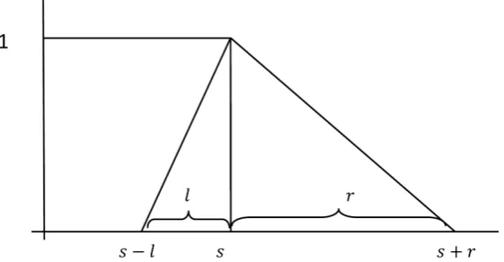
Definition 2.8: A fuzzy number a on R is said to be triangular fuzzy

num-ber, if there exist real numbers and l r, ≥0 such that

( )

[

]

[

]

, ,

0, o.w.

x l s

x s l s

l l

a x x s r

x s s r

r r

−

 + ∈ −

 

= −_ +

+ ∈ +

   

We denote a triangular fuzzy number a by three real numbers s l, and r as a= s l r, , , whose meaning are defined in Figure 1. We also denote the set

of all triangular fuzzy numbers with F(R).

Definition 2.9: Let a= s l r_a, ,_a _a and b= s lb, ,b rb be two triangular

num-bers and x∈R. Summation and multiplication of fuzzy numbers defined as [18]:

, , , 0

a a a

xs xl xr x

x xs a

xr xl x

 ≥

 = 

− − <

(4)

[image:4.595.237.518.73.219.2]

Figure 1. Fuzzy Triangular Number.

, ,

a b a b a b

s s l

a+ =b + +l r +r

, ,

a b a b a b

s s l

a− =b − −r r −l

a≤b if and only if sa≤s sb, a− ≤ −la sb l sb, a+ ≤ +ra sb rb

Definition 2.10: We let 0=

(

0, 0, 0

)

as a zero triangular fuzzy number. Remark 2.1: a ≥0 if and only if sa≥0,sa− ≥la 0,sa+ ≥ra 0.

Remark 2.2: a≤b if and only if − ≥ −a b.

3. Fuzzy Numbers Quadratic Programming

Here we first define the model and then propose a novel method for solving the mentioned problem.

3.1. Definition of Model

Several studies have developed efficient and effective algorithms for solving qu-adratic programming when the value assigned to each parameter is a known constant. However, quadratic programming models usually are formulated to find some future course of action so the parameter values used would be based on a prediction of future conditions which inevitably involves some degree of uncertainty [19][20]. The most general type of this programming is formulated as follows:

1 1 1

1

1 max

2

, ,

s.t. 0

n n n

j j ij i j

j i j

n

ij j i m

j

C X X X

B

z Q

A X i

X

N

= = =

=

= +

 _≤ _∈

   ≥ 

∑

∑∑

∑

   



  (3.1)

where Aij, Bi, Cj and Qij are fuzzy numbers, and Xj are variables whose

states are fuzzy numbers

(

i∈N_m,j∈N_n

)

; the operations of addition and

(5)

1 1 1

1 1 max 2 , , s.t. 0

n n n

j j ij i j

j i j

n

ij j i m

j

B

x

z c x q x x

A x i N

= = = = = +  ≤ ∈    ≥ 

∑

∑∑

∑

  (3.2)

3.2. The New Approach

In this case we assume that all fuzzy numbers are triangular. According to Defi-nition 2.8, the fuzzy quadratic programming (3.2) is rewritten as follows:

1 1 1

1 1 max 2 , , , , , s.t. 0,

n n n

j j ij i j

j i j

n

ij ij ij j i i i m

j

j n

z c x q x x

a l r x b u v i N

x j N

= = = = = +  ≤ ∈    ≥ ∈ 

∑

∑∑

∑

(3.3)

where A_ij = a l r_ij, ,_ij _ij and Bi= b u vi, ,i i are fuzzy numbers. According to

Definition 2.9, the constraint 1 , , , , ,

n

ij ij ij j i i i m

j= a l r x ≤ b u v i∈N

∑

yields that:

(

)

(

)

1 1 1

, and ,

n n n

ij j i ij ij j i i ij ij j i i m

j j j

a x b a l x b u a r x b v i N

= = =

≤ − ≤ − + ≤ + ∈

∑

Substituting these relations in to (3.3) the conventional quadratic program is derived as follows:

(

)

(

)

1 1 1

1 1 1 1 max 2 , , , 0,

n n n

j j ij i j

j i j

n

ij j i m

j n

ij ij j i i m

j n

ij ij j i i m

j

j n

z c x q x x

a x b i N

a l x b u i N

a r x b v i N

x j N

= = = = = = = + ≤ ∈ − ≤ − ∈ + ≤ + ∈ ≥ ∈

∑

∑∑

∑

(3.4)

However, since all numbers involved are real numbers, this is classical qua-dratic programming problem which can be solved using MATLABTM_toolbox. The SQP algorithm is used as an optimization method to minimize the nonli-near constrained optimization problem. This method is described as follow:

3.3. The SQP Algorithm

(6)

optimization problem in the SQP method is considered as follows:

( )

minimize

subjected to : i 0, 1, ,

J x

x i m

ψ ≤ =  (3.5)

where J x

( )

is the cost function and ψ_i

( )

x stands for the constraint. In this

regard a Lagrangian function L x

( )

,λ is constructed in terms of the Lagrangian

multiplier λi. The cost function together with the above constraint is defined as

follows:

(

)

( )

1 , m i i i

L xλ J x λψ x

=

= +

∑

_(3.6)

In fact the SQP consists of three main parts:

1- Update the Hessian of the Lagrangian function according to:

(

)

(

)

( )

T T

1 T T

0 1

1 1

k k k k

k k

k k k k k

k k k

n n

k k i i k k i i k

i i

q q H H

H H

q S S H S

H I

S X X

q f X λ g X f X λ g X

+ + + + = = = + − = = −   = ∇ + ∇ − ∇_ + ∇ _  

∑

(3.7)

2- Solve the quadratic programming sub-problem:

( )

T T T T 1 min 2

0, 1, , 0, 1, ,

k k k k k

i k k i k

q H d f x d

x d x i m

ψ

+ ∇ ∇ + = = ∇ + ≥ =   (3.8)

3- A linear search to find a solution for the next iteration:

1

k k k

X + =X +αd (3.9)

The algorithm is repeated until a stopping criterion (either maximum itera-tion or convergence criterion) is met. It must be menitera-tioned that the SQP algo-rithm is a gradient based algoalgo-rithm. Generally gradient based methods have the possibility of getting trapped at local optimum depending on the initial guess of the solution. In order to achieve a good final result, these methods require very good initial guesses of the solution. Since the matrix Q is supposed symmetric

(

qij=qji

)

and semidefinite, the objective function is convex and thus the SQP

algorithm yields the global optimum solution. The corresponding theorem is presented as follows:

Theorem 3.1: In mathematical terminology, f x x

(

1, 2,,xn

)

is convex if and

only if its n n× Hessian matrix is positive semi definite for all possible values of

(

x x1, 2,,xn

)

. That is for any x≥0 the following relation is satisfied:

(

)

(

)

2 2 1 2 1 1 2

1 2 1 2

2 2

2 1

, , , 0, , , ,

n n n n n n n f f x x x x x

x x x x x x

f f

x

x x x

(7)

in which

( )

2 2

2

1

1 ₂

2 2

2 1

n

j i _{n n}

n n

f f

x x x

f H x

x x

f f

x x x

×

 ∂ ∂ 

 _∂ _{∂ ∂} 

 _{ } _∂ _

 

=_ _=  

∂ ∂

 

 

∂ ∂

 

_{∂ ∂} _∂ 

 



  



is the Hessian matrix of

function f . Hence the above relation can be rewritten as follow:

( )

T

0, n

x H x x≥ ∀ ∈x 

Proof: See in [26].

4. An Example

In this section, we utilize an example to illustrate the solution method proposed in this paper. Consider a river from which diversions are made to three water- consuming firms that belong to the same corporation, as illustrated in Figure 1

Each firm makes a product, and is the critical resource. Water is needed in the process of making that product, and it is critical resource. The three firms can be denoted by the index j=1, 2, 3 and their water allocations by xj. Assume the

problem is to determine the allocations xj of water to each of three firms

(

j=1, 2, 3

)

that maximize the total net benefits,

∑

jNBj

( )

xj , obtained from

all three firms. The total amount of water available is constrained or limited to a quantity of Q. Assume the net benefits NBj

( )

xj , derived from water xj

allo-cated to each firm j, are defined by:

( )

2 1 1 1 0.5 1

NB x = +x x (4.1)

( )

2 2 2 2 2 2

NB x = x +x (4.2)

( )

2 3 3 3 1.5 3

NB x =x + x (4.3)

The problem is to find the allocations of water to each firm that maximize the total benefits TB X

( )

:

( )

1

( )

1 2

( )

2 3

( )

3

TB X =NB x +NB x +NB x (4.4)

These allocations cannot exceed the amount of water available, Q, less any that must remain in the river, R. Assuming the available flow for allocations,

Q−R, is 4. The crisp optimization problem is to maximize Equation (4.4)

sub-ject to the resource constraint:

1 2 3 4

x +x +x ≤ (4.5)

Thus the problem is:

( )

(

2

) (

2

) (

2

)

1 1 2 2 3 3

1 2 3

max 0.5 2 1.5

4 s.t.

, , 0

TB X x x x x x x

x x x

x x x

= + + + + +

+ + ≤



 _≥



(4.6)

(8)

or fuzzy. If the values are uncertain, probability distributions may be used to quantify them. Alternatively, if they are best described by qualitative adjectives, such as dry or wet, hot or cold, clean or dirty, and high or low, fuzzy member-ship function can be used to quantify them. Both probability distribution and fuzzy membership functions of these uncertain or qualitative variables can be included in quantitative optimization models. Now we illustrate how fuzzy de-scriptors can be incorporated into optimization models of water resources sys-tems. Assuming the available flow for allocations, Q−R, is not certainly known

and is represented by an interval 4, 2,1.5 . Thus the problem turns to the fuzzy

quadratic programming problem as follows:

( )

(

2

) (

2

) (

2

)

1 1 2 2 3 3

1 2 3

max 3 2 1.5

4, 2,1.5 s.t.

, , 0

TB X x x x x x x

x x x

x x x

= + + + + +

 + + ≤



 _≥



(4.7)

This problem is in the form of model (3.2). Hence it can be solved using the proposed method. Since the parameter b1, is triangular fuzzy number, thus the objective value of the problem should be fuzzy number as well. According to the proposed method the fuzzy solution obtained by solving the following program:

( )

(

2

) (

2

) (

2

)

1 1 2 2 3 3

1 2 3

max 3 2 1.5

4 2 s.t.

5.5

, , 0

TB X x x x x x x

x x x

x x x

= + + + + +

+ + ≤ 

 + + ≤ 

 + + ≤ 

 _≥



where parameter values are all known constant. Thus this model is conventional quadratic programming problems. By solving this problem using SQP algorithm the global optimum solution is obtained as:

(

2, 0, 0

)

X =

The value of objective function is also achieved *

10

z = .

5. Conclusion

(9)

Our other suggestion is establishing a new rule for fuzzy ordering.

Acknowledgements

The authors would like to thank the anonymous referees for their valuable comments that help us to improve the earlier version of this work.

References

[1] Floudas C.A., Pardalos P., Adjiman C., Esposito W.R., Gumus Z.H., Harding S.T., Klepeis J.L., Meyer C.A. and Sshweiger, C.A. (1999) Handbook of Test Problems in Local and Global Optimization. Non convex Optimization and its Applications, Vol. 33, Kluwer Academic Publishers, Dordrecht.

[2] Gould, N.I.M. and Toint, P.L. (2000) A Quadratic Programming Bibliography. RAL Numerical Analysis Group Internal Report 2000-1, Department of Mathematics, University of Namur, Bruxelles, Belgium.

[3] Hock, W. and Schittkowski, K. (1981) Test Examples for Nonlinear Programming Codes. Lecture Notes in Economics and Mathematical Systems, Vol. 187, Spring-Verlag, Berlin.

[4] Maros, I. and Meszaros, C. (1997) A Repository of Convex Quadratic Problems. Department Technical Report DOC 97/6, Department of Computing, Imperial Col-lege, London, UK.

[5] Schittkowski, K. (1987) More Test Examples for Nonlinear Programming Codes. Lecture Notes in Economics and Mathematical Systems, Vol. 282, Spring-Verlag, Berlin.

[6] Beale, E. (1959) On Quadratic Programming. Naval Research Logistics Quarterly, 6, 227-244.https://doi.org/10.1002/nav.3800060305

[7] Bellman, R.E. and Zadeh, L.A. (1970) Decision-Making in a Fuzzy Environment.

Management Science, 17, 164.https://doi.org/10.1287/mnsc.17.4.B141 [8] Markowitz, H. (1952) Portfolio Selection. The Journal of Finance, 7, 77-91. [9] Markowitz, H.M. (1991) Portfolio Selection: Efficient Diversification of

Invest-ments. 2nd Edition, Blackwell Publisher.

[10] Inuiguchi, M. and Ramik, J. (2000) Possibilistic Linear Programming: A Brief Re-view of Fuzzy Mathematical Programming and a Comparison with Stochastic Pro-gramming in Portfolio Selection Problem. Fuzzy Sets and Systems, 111, 3-28. [11] Leon, T. and Liercher, E. (2000) Viability of Infeasible Portfolio Selection Problems:

A Fuzzy Approach. European Journal of Operational Research, 139, 178-189. [12] Tanaka, H., Guo, P. and Turksen, B. (2000) Portfolio Selection Based on Fuzzy

Probabilities and Possibility Distributions. Fuzzy Sets and Systems, 111, 387-397. [13] Verchur, E., Bermudez, J.D. and Segura, J.V. (2007) Fuzzy Portfolio Optimization

under Downside Risk Measures. Fuzzy Sets and Systems, 158, 769-782.

[14] Watada, J. (1997) Fuzzy Portfolio Selection and Its Applications to Decision Mak-ing. Tatra Mountains Mathematics Publications, 13, 219-248.

[15] Mahdavi-Amiri, N., Nasseri, S.H. and Yazdani Cherati, A. (2009) Fuzzy Primal Simplex Algorithm for Solving Fuzzy Linear Programming Problems. Iranian Jour-nal of OperatioJour-nal Research, 2, 68-84.

(10)

Jour-DOI: 10.4236/jamp.2017.511181 2227 Journal of Applied Mathematics and Physics

nal of Industrial Engineering, 4, 327-389.https://doi.org/10.1504/EJIE.2010.033336 [17] Nasseri, S.H. and Mahdavi-Amiri, N. (2009) Some Duality Results on Linear

Pro-gramming Problems with Symmetric Fuzzy Numbers. Fuzzy Information and En-gineering, 1, 59-66.https://doi.org/10.1007/s12543-009-0004-2

[18] Nasseri, S.H., Attari, H. and Ebrahimnejad, A. (2012) Revised Simplex Method and Its Application for Solving Fuzzy Linear Programming Problems. European Journal of Industrial Engineering, 6, 259-280.https://doi.org/10.1504/EJIE.2012.046670 [19] Lio, S.T. (2009) Quadratic Programming with Fuzzy Parameters. Chaos, Solitons

and Fractals, 40, 237-245.

[20] Lio, S.T. (2009) A Revisit to Quadratic Programming with Fuzzy Parameters.

Chaos, Solitons and Fractals, 41, 1401-1407.

[21] Modares, H. and NaghibiSistani, M.B. (2011) Solving Nonlinear Optimal Control Problems using a Hybrid IPSO-SQP Algorithm. Journal of Engineering Applica-tions of Artificial Intelligence, 24, 476-484.

[22] Bayon, L., Grau, J.M., Ruiz, P.M. and Suarez, M.M. (2010) Initial Guess of the Solu-tion of Dynamic OptimizaSolu-tion of Chemical Processes. Journal of Mathematical Chemistry, 48, 27-38.https://doi.org/10.1007/s10910-009-9614-5

[23] Costa, C.B.B., Maciel, A.C. and Filho, R. (2005) Mathematical Modeling and Op-timal Control Strategy Development for an Acidic Crystallization Process. Chemical Engineering and Processing, 44, 737-753.

[24] Hu, G. and Xu, S. (2009) Optimization Design of Microchannel Heat Sink Based on SQP Method and Numerical Simulation. Applied Conference on Superconductivity and Electromagnetic Devises, ASEMD, 89-92.

[25] Wang, R., Wang, P. and Zhu, Y. (2011) Study on Optimization of Isolated Heat Pipe Heat Exchange System Based on SQP. International Conference on Electric Infor-mation and Control Engineering.

http://www.scirp.org/journal/jamp

: 10.4236/jamp.2017.511181

http://creativecommons.org/licenses/by/4.0/

4.

https://doi.org/10.1287/mnsc.17.4.B141

https://doi.org/10.1504/EJIE.2010.033336

66.

https://doi.org/10.1504/EJIE.2012.046670

https://doi.org/10.1007/s10910-009-9614-5