Crowdsourced Word Sense Annotations
and Difficult Words and Examples
Oier Lopez de Lacalle University of the Basque Country
Eneko Agirre
University of the Basque Country
Abstract
Word Sense Disambiguation has been stuck for many years. The recent availability of crowd-sourced data with large numbers of sense annotations per example facilitates the exploration of new perspectives. Previous work has shown that words with uniform sense distribution have lower accu-racy. In this paper we show that the agreement between annotators has a stronger correlation with performance, and that it can also be used to detect problematic examples. In particular, we show that, for many words, such examples are not useful for training, and that they are more difficult to disam-biguate. The manual analysis seems to indicate that most of the problematic examples correspond to occurrences of subtle sense distinctions where the context is not enough to discern which is the sense that should be applied.
1 Introduction
Word sense ambiguity is a major obstacle for accurate information extraction, summarization and ma-chine translation, but there is still a lack of high performance Word Sense Disambiguation systems (WSD). The current state-of-the-art is around the high 60s accuracy for words in full documents (Zhong and Ng, 2010), and high 70s for words with larger number of training examples (lexical sample). The lack of large, high-quality, annotated corpora and the fine-grainedness of the sense inventories (typi-cally WordNet) are thought to be the main reasons for the poor performance (Hovy et al., 2006). The situation of WSD is in stark contrast to the progresses made on Named-Entity Disambiguation, where performance over 80% accuracy is routinely reported (Hoffart et al., 2012).
In this paper we focus on the recent release of crowdsourced data with large numbers of sense anno-tations per example (Passonneau and Carpenter, 2014), and try to shed some light in the factors that affect the performance of a supervised WSD system. In particular, we extend the analysis set up in (Yarowsky and Florian, 2002), and show that the agreement between annotators has a strong correlation with the performance for a particular word, stronger than previously used factors like the number of senses of the word and the sense distribution for the word.
In addition, we show that crowdsourced data can be used to detect problematic examples. In particu-lar, our results indicate that, for many words, such examples are not useful for training, and that they are more difficult to disambiguate. The last section shows some examples.
2 Previous work on factors affecting WSD performance
WSD is a problem which differs from other natural language processing tasks in that each target word is a different classification problem, in contrast to, for instance, document classification, PoS tagging or parsing, where one needs to train one single classifier for all. Furthermore, it is already known that, given a fixed amount of training data, the performance of a supervised WSD algorithm varies from one word to another (Yarowsky and Florian, 2002).
Yarowsky and Florian (2002) did a thorough analysis of the behaviour of several WSD systems on a variety of factors: (a) target language (English, Spanish, Swedish and Basque); (b) part of speech; (c)
sense granularity; (d) inclusion and exclusion of major feature classes; (e) variable context width (further broken down by part-of-speech of keyword); (f) number of training examples; (g) baseline probability of the most likely sense; (h) sense distributional entropy; (i) number of senses per keyword; (j) divergence between training and test data; (k) degree of (artificially introduced) noise in the training data; (l) the effectiveness of an algorithms confidence rankings. Their analysis was based on the annotated examples for a handful of words, as released in the SensEval2 lexical sample task (Edmonds and Cotton, 2001).
In particular they found that the performance of all systems decreased for words with higher number of senses (as opposed to words with few senses) and for those with more uniform distributions of senses (as opposed to words with skewed distributions of senses). The distribution of senses was measured using the entropy of the probability distribution of the senses, normalized by the number of senses1
Hr(P) = H(P)/log2(#senses), where H(P) = −Pi∈sensesp(i)log2p(i) (Yarowsky and Florian,
2002).
In this paper we quantify the correlation of those two factors with the performance of a WSD system, in order to compare their contribution. In addition, we analyse a new factor, agreement between annota-tors, which can be used not only to know which words are more difficult, but also to characterize which examples are more difficult to disambiguate. To our knowledge, this is the first work which quantifies the contribution of each of these factors towards the performance on WSD, and the only one which analyses example difficulty for WSD on empirical grounds.
Our work is also related to (Plank et al., 2014), which showed that multiple crowdsourced annotations of the same item allow to improve the performance in PoS tagging. They incorporate the uncertainty of the annotators into the loss function of the model by measuring the inter-annotator agreement on a small sample of data, with good results. Our work can be seen as preliminary evidence that such a method can be also applied to WSD.
3 Measuring annotation agreement
The corpus used in the experiments is a subset of MASC, the Manually Annotated Sub-Corpus of the Open American National Corpus (Ide et al., 2008), which contains a subsidiary word sense sentence corpus consisting of approximately one thousand sentences per word annotated with WordNet 3.0 sense labels (Passonneau et al., 2012). In this work we make use of a publicly available subset of 45 words (17 nouns, 19 verbs and 9 adjectives, see Table 4) that have been annotated, 1000 sentences per target word, using crowdsourcing (Passonneau and Carpenter, 2014). The authors collected between 20 and 25 labels for every sentence.
We measured annotation agreement using the multiple annotations in the corpus and calculate the annotation entropy of an example and word sense distribution entropy as follows. In annotation entropy, we use directly the true-category probabilities from Dawid and Sekene’s model (Passonneau and Car-penter, 2014) associated to each example to measure its entropy (as defined in the previous section). The annotation entropy for a word is the average of the entropy for each example. In sense entropy, on the other hand, we measure the overall confusion among senses and based on confusion distribution we cal-culate the entropy of each word sense. Similarly, the sense entropy of a word is averaged over all word sense entropy measures.
4 Annotation agreement explains word performance
We created a gold standard with a single sense per example, following (Passonneau and Carpenter, 2014), which use a probabilistic annotation model (Dawid and Skene, 1979). We split the 1000 examples for each word into development and test, sampling 85% (and 15% respectively) at random, preserving the overall sense distribution.
1The normalization ensures that the figure is comparable across words, as we divide by the maximum entropy for a word
● ● ● ● ● ● ● ● ● ● ● ● ● ● ● ● ● ● ● ● ● ● ● ● ● ● ● ● ● ● ● ● ● ● ● ● ● ● ● ● ● ● ● ● ● pearson: −0.26 40 60 80
5.0 7.5 10.0 12.5 15.0 17.5
Number of senses
Fscore ● ● ● ● ● ● ● ● ● ● ● ● ● ● ● ● ● ● ● ● ● ● ● ● ● ● ● ● ● ● ● ● ● ● ● ● ● ● ● ● ● ● ● ● ● pearson: −0.35 40 60 80
0.4 0.6 0.8
Sense entropy Fscore ● ● ● ● ● ● ● ● ● ● ● ● ● ● ● ● ● ● ● ● ● ● ● ● ● ● ● ● ● ● ● ● ● ● ● ● ● ● ● ● ● ● ● ● ● pearson: −0.38 40 60 80
0.00 0.05 0.10
Annotation entropy
[image:3.595.78.523.76.218.2]Fscore
Figure 1: Scatterplots that show the correlation between the factors and accuracy. Each point corresponds to a word.
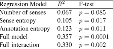
Regression Model R2 F-test
Number of senses 0.067 p= 0.085
Sense entropy 0.105 p= 0.017
Annotation entropy 0.123 p= 0.011
Full model 0.357 p= 0.0001
[image:3.595.204.393.257.339.2]Full interaction 0.330 p= 0.002
Table 1: Regression analysis summary. The first three rows refer to the simplest models, where each factor (annotation entropy, sense entropy and number of senses) is taken in isolation. The full model takes all three factors with no interaction, and the full interaction includes all three factors and interactions.
R2and F-test indicate whether the model is fitted.
The Word Sense Disambiguation algorithm of choice isIt Makes Sense(IMS) (Zhong and Ng, 2010), which reports the best WSD results to date. We used it out-of-the-box, using the default parametrization and built-in feature extraction. The system always returned an answer, so the accuracy, precision, recall and F1 score are equal.
As explored in (Yarowsky and Florian, 2002), the variability of the accuracy across words can be related to many factors, including the distribution of senses and the number of senses of the word in the dataset. In this work, we introduce annotation agreement to the analysis. Figure 1 shows how each factor is correlated with the performance of the IMS WSD system, along with the Pearson product-moment. The highest correlation with the performance is for annotation entropy (-0.38) and the lowest for the number of senses (-0.26), whilst sense entropy has slightly lower correlation (-0.35) than annotation entropy.
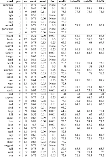
Table 4 shows the number of senses, entropy of sense distribution and the entropy of the annotation agreement for each of the 45 target words.
In addition, we performed regression analysis of the three factors, alone, and in combination. All in all, we fit 5 linear models: the simplest models take each factor alone in a simple linear model;2 the
full model uses the three factors as a linear combination with no interaction between the factors; the full interaction model also models pairwise and three-wise multiplications of the factors.3
Table 1 shows the main figures of the analysis. Regarding models with only one factor, the entropy of annotation agreement explains performance better than sense entropy and number of senses (the higher
R2the better the model fits the data). Actually, the number of senses alone is not a significant factor that
explains the difficulty of a word (t-testp >0.05), although in combination with the other factors it is a valuable information. Annotation agreement and the sense distribution do have a significant correlation according to the t-test.
2The simplest linear regression model is typically formalized as follows:f=B0+B1·factor i+ 3This can be generalized as follows:f=B0+P
iBi·factori+
P
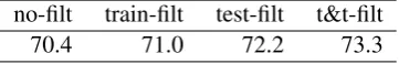
no-filt train-filt test-filt t&t-filt 70.4 71.0 72.2 73.3
Table 2: Average results for the 30 words which get improvement using thresholds. Legend (cf. Section 5): no-filt for using full train and test data, train-filt for filtered train, test-filt for filtered test, and t&t-filt for filtered train and test. See table 4 for statistics and results of individual words.
The results for the “full model” show that the three models are complementary, and that in combi-nation they account for 35.7% of the variance of the WSD performance measured in Fscore (according to adjusted R2), with high significance. The analysis shows, as well, that the “full interaction” model
does not explain the performance any better. Although this model is also significant (F-testp= 0.002), the adjustedR2 is lower than in the “full model” (0.357vs0.330), showing that combining the factors
without interactions is sufficient.4
5 Annotation agreement characterizes problematic examples
Contrary to the sense distribution of a word, annotation agreement can be used to detect problematic examples. In particular, we show that, for many words, such examples are not useful for training, and that they are more difficult to disambiguate.
We explored the use of thresholds to ignore the training examples with highest annotation entropy per example. 15% of the train data was set aside for development, and the rest was used to train IMS. We tried several thresholds: 0.5,0.25,0.1,0.05,0.01,0.001. The lower the threshold the fewer examples to train (difficult examples have high entropy values). Table 4 in the appendix shows the thresholds which yield the best results on development data. Overall, In 15 out of the 45 words, the best results on development were obtained using all the data, but for the remaining 30, removing examples improved results on development. Incidentally, those 15 words tend to have lower annotation entropy than the 30 words.
Table 2 shows the results on test data for the 30 words that improve on development. The train-filt column shows the results when we remove the examples with less agreement from train. Note that the threshold was only applied to 30 words. The performance improvement over using the full train data is on 0.6 absolute for these 30 words. The improvement is concentrated on 12 words, as 9 words get equal, and 9 words get a decrease in performance. When we use the threshold set in development to remove examples with less agreement from test, the performance increases 1.8 (test-filt column in Table 2). In this case, 23 words get better performance, 4 equal, and 3 words get a decrease. Finally, when we train and test on examples below the threshold, the improvement on the 30 words amount to 2.9. 24 words get better performance, 4 equal, and only 2 words get a decrease.
6 Examples
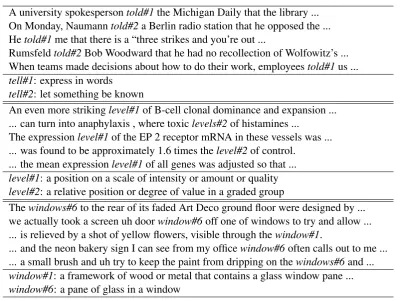
We sampled some problematic examples for the three words which attain the best improvement when removing examples from train with respect to the baseline: tell,levelandwindow, in this order. Table 3 shows the 5 examples with highest annotation entropy for tell. The examples correspond to uses oftell where two fine-grained distinctions in WordNet5 are hard to differentiate. A similar trend was
observed for levelandwindow(cf. Table 3), where the examples with high annotation entropy where also annotated with two fine-grained closely related senses. In all three words the examples corresponded to the two most frequent senses.
We had hypothesized two factors which could explain the high annotation entropy for some exam-ples: the confusability among two senses of the word, and poor context for disambiguation. The manual
A university spokespersontold#1the Michigan Daily that the library ... On Monday, Naumanntold#2a Berlin radio station that he opposed the ... Hetold#1me that there is a “three strikes and you’re out ...
Rumsfeldtold#2Bob Woodward that he had no recollection of Wolfowitz’s ... When teams made decisions about how to do their work, employeestold#1us ...
tell#1: express in words
tell#2: let something be known
An even more strikinglevel#1of B-cell clonal dominance and expansion ... ... can turn into anaphylaxis , where toxiclevels#2of histamines ...
The expressionlevel#1of the EP 2 receptor mRNA in these vessels was ... ... was found to be approximately 1.6 times thelevel#2of control.
... the mean expressionlevel#1of all genes was adjusted so that ...
level#1: a position on a scale of intensity or amount or quality
level#2: a relative position or degree of value in a graded group
Thewindows#6to the rear of its faded Art Deco ground floor were designed by ... we actually took a screen uh doorwindow#6off one of windows to try and allow ... ... is relieved by a shot of yellow flowers, visible through thewindow#1.
... and the neon bakery sign I can see from my officewindow#6often calls out to me ... ... a small brush and uh try to keep the paint from dripping on thewindows#6and ...
window#1: a framework of wood or metal that contains a glass window pane ...
[image:5.595.99.502.65.366.2]window#6: a pane of glass in a window
Table 3: Five examples with highest annotation entropy fortell,levelandwindow, annotated with senses. Corresponding definitions are also given.
inspection seems to indicate the the former is the main factor in play here, confounded by the fact that the context does not allow to properly distinguish the specific sense, leaving it underspecified.
7 Conclusions and future work
The recent availability of crowdsourced data with large numbers of sense annotations per example allows to explore new perspectives in WSD. Previous work has shown that words with uniform sense distribu-tion have lower accuracy. In this paper we show that the agreement between annotators has a stronger correlation with performance, and that it can be used to detect problematic examples. In particular, we show that, for many words, such examples are not useful for training, and that they are more difficult to disambiguate. Manual analysis seems to indicate that most of the problematic examples correspond to occurrences of subtle sense distinctions, where the context is not enough to discern which is the sense that should be applied.
In the future, we would like to explore methods that exploit problematic examples. On the one hand removing problematic examples could improve sense clustering, and vice-versa, clustering could help reduce the number of problematic examples. On the other hand detecting problematic examples could be used to improve WSD systems, for instance, using more refined ML techniques like Plank et al. (2014) to treat low agreement examples sensibly, or detecting underspecified examples in test.
Acknowledgements
References
Dawid, A. P. and A. M. Skene (1979). Maximum likelihood estimation of observer error-rates using the em algorithm.Applied Statistics 28(1), 20–28.
Edmonds, P. and S. Cotton (2001). Senseval-2: Overview. In The Proceedings of the Second Interna-tional Workshop on Evaluating Word Sense Disambiguation Systems, SENSEVAL ’01, Stroudsburg, PA, USA, pp. 1–5. Association for Computational Linguistics.
Hoffart, J., S. Seufert, D. B. Nguyen, M. Theobald, and G. Weikum (2012). Kore: Keyphrase overlap relatedness for entity disambiguation. InProceedings of the 21st ACM international conference on Information and knowledge management, pp. 545554.
Hovy, E., M. Marcus, M. Palmer, L. Ramshaw, and R. Weischedel (2006). Ontonotes: The 90 In Pro-ceedings of HLT-NAACL 2006, pp. 57–60.
Ide, N., C. Baker, C. Fellbaum, C. Fillmore, and R. Passonneau (2008, may). MASC: the Manually Annotated Sub-Corpus of American English. InProceedings of the Sixth International Conference on Language Resources and Evaluation (LREC’08), Marrakech, Morocco. European Language Re-sources Association (ELRA). http://www.lrec-conf.org/proceedings/lrec2008/.
Passonneau, R. J., C. F. Baker, C. Fellbaum, and N. Ide (2012, may). The MASC word sense corpus. In N. C. C. Chair), K. Choukri, T. Declerck, M. U. Doan, B. Maegaard, J. Mariani, A. Moreno, J. Odijk, and S. Piperidis (Eds.), Proceedings of the Eight International Conference on Language Resources and Evaluation (LREC’12), Istanbul, Turkey. European Language Resources Association (ELRA). Passonneau, R. J. and B. Carpenter (2014). The benefits of a model of annotation. Transactions of the
Association for Computational Linguistics 2(1-9), 311–326.
Plank, B., D. Hovy, and A. Søgaard (2014, April). Learning part-of-speech taggers with inter-annotator agreement loss. InProceedings of the 14th Conference of the European Chapter of the Association for Computational Linguistics, Gothenburg, Sweden, pp. 742–751. Association for Computational Linguistics.
Yarowsky, D. and R. Florian (2002). Evaluating sense disambiguation across diverse parameter spaces.
Natural Language Engineering 8(4), 293–310.
Appendix: statistics for individual words
word pos ns s-ent a-ent thr no-filt train-filt test-filt t&t-filt
common j 1 0.72 0.03 None 70.5
fair j 11 0.45 0.00 0.1 88.8 89.8 88.8 89.8
full j 9 0.63 0.11 0.5 78.5 77.8 78.6 78.6
high j 8 0.55 0.01 None 86.3
late j 8 0.71 0.00 None 84.9
long j 1 0.49 0.01 None 78.0
normal j 5 0.71 0.05 0.5 81.9 79.9 82.3 80.1
particular j 7 0.82 0.05 None 85.0
poor j 6 0.75 0.06 None 76.2
board n 1 0.32 0.00 0.001 88.9 88.9 89.5 89.5
book n 12 0.43 0.05 0.5 56.3 56.3 58.3 58.3
color n 9 0.73 0.13 0.25 65.5 66.2 68 69.7
control n 12 0.72 0.01 None 79.5
date n 9 0.85 0.02 0.25 80.1 80.1 80.4 81.2
family n 9 0.73 0.04 0.001 64.3 64.3 64.8 66.7
image n 1 0.65 0.01 None 70.6
land n 12 0.81 0.02 None 57.6
level n 9 0.57 0.07 0.05 70.5 71.9 70.4 77.8
life n 15 0.82 0.01 0.5 58 58.7 58 58.7
number n 12 0.41 0.01 0.25 87.7 87.7 87.6 87.6
paper n 8 0.74 0.05 0.05 76.4 75 78 76.3
sense n 6 0.78 0.00 None 93.8
time n 11 0.64 0.01 0.25 89.6 88.5 90.0 88.9
way n 13 0.56 0.05 None 72.8
window n 5 0.8 0.02 0.05 75.9 78.6 77.4 80.3
work n 8 0.95 0.02 0.001 69.8 66.3 75.9 74.1
add v 7 0.77 0.03 0.01 41 41 41 41
appear v 8 0.75 0.11 0.25 64.4 63 68.5 67.7
ask v 8 0.61 0.08 0.01 78.3 76.2 86.7 86.7
find v 17 0.69 0.05 0.01 62.4 64.5 65.8 67.5
fold v 6 0.38 0.01 None 93.2
help v 9 0.69 0.09 0.001 61.2 64 67.1 71.4
kill v 16 0.52 0.01 0.001 63.9 66.7 65 67.9
know v 12 0.66 0.09 0.5 63.1 67.2 63.9 68.3
live v 8 0.81 0.00 0.001 73.5 74.8 74.1 75.5
lose v 12 0.7 0.01 0.001 64.4 64.4 67.2 66.4
meet v 14 0.77 0.02 0.5 69.7 69 69.7 69
read v 12 0.46 0.00 None 82.8
say v 12 0.66 0.05 0.1 64.9 64.9 68.7 69.5
serve v 16 0.71 0.01 0.5 73.1 73.1 72.9 72.9
show v 13 0.66 0.03 None 76.2
suggest v 5 0.71 0.04 None 74.3
tell v 9 0.73 0.1 0.1 57.6 65.3 59.8 65.7
wait v 5 0.82 0.07 0.5 69.5 74 71.1 76
[image:7.595.113.482.109.658.2]win v 9 0.72 0.08 0.05 72.8 72.1 76.3 77.2