Procurement Contracts under Limited Liability
Abstract:This paper analyses procurement when contractors have limited liability and when the sponsor cannot commit to any specific form of future negotiation. It shows that introducing limited liability enhances competition and thus the likelihood of bankruptcy. Among efficient auctions in which only the winner gets paid, the commonly used first price auction is shown to give the lowest probability of bankruptcy. Finally, it shows that the characterisation of a mechanism minimising the project’s cost results from trading-off bankruptcy costs with informational rents.
I INTRODUCTION
I
n procurement contracting, tenders must generally be submitted at a stage where there is still much uncertainty. Part of this uncertainty results from possible imperfect information regarding future costs or the exact characteristics of the product to be supplied. Another part is potentially associated with the sponsor being unable, or even unwilling, to commit to any specific future negotiation in the event of cost overruns. Indeed, the type of agreements that can be made in practice are often limited.Under these circumstances, costs estimates and the level of liability are the only factors contractors can rely on when submitting tenders. Thus, in the absence of any form of future agreements, limited liability plays a crucial role as it determines the extent to which a contract can be enforced. It is then important, for those who decide on procurement rules, to understand how
1
* I am grateful to Roberto Burguet, Jacques Crémer, Kaï-Uwe Kuhn, Donal O’Neill, Fabrice Rousseau, and particularly to an anonymous referee for their comments.
SARAH PARLANE*
limited liability constraints affect the contractors’ initial bidding decisions, as well as the outcome (e.g. the contracted price, the likelihood of bankruptcy) of the rules they set. This paper examines bidding under limited liability in the absence of specific future agreements. It highlights some possible consequences of limited liability constraints and compares the performance of different procurement rules. Although the analysis relies on a theoretical model, the results are informative from an applied point of view and of potential interest to policy makers.
In the literature, limited liability is often introduced as an ex post voluntary participation constraint. Formally, it states that the contract cannot be enforced whenever the contractor’s profit falls below a certain level. Its implications then depend on the sponsor’s ability and willingness to enforce the contract. In Riordan and Sappington (1988), the sponsor can either use contingent prices,1or can commit to negotiate a price in a second period, once all uncertainty is resolved. Contingent prices are set such that bankruptcy will not arise. Thus, they eliminate the possible distortions resulting from facing a potentially binding limited liability constraint. Unfortunately, in practice, it is often impossible for the sponsor to anticipate all future contingencies and therefore to write and rely on complete contracts. Without this possibility, limited liability constraints are likely to have a greater impact. When the price is negotiated ex post, an auction is used in a first period to select a contractor. To prevent the submission of very low tenders that would decrease the first period rent and make it impossible for the contractor to cover his cost, a minimal acceptable bid is imposed. These authors then show that the limited liability constraints then hold at the expense of efficiency. Indeed, in some cases, all contractors submit the minimal acceptable bid in the auction (this forms a so-called pooling equilibrium). In such a case, the auction does not allow one to identify and select the most efficient contractor. Committing to future negotiations is not always feasible and more importantly, not always desirable. A sponsor may not want to be locked in with a contractor who may then take advantage of the situation to increase his costs. Moreover, setting a minimal acceptable bid usually requires some information regarding future possible costs, the evolution of the project and so on. This is not always available to the sponsor. The following analysis discards both, the use of complete contracts and the possibility to commit to any specificform of future negotiation.
If all competitors have the same operating cost but differ in the level of their potential cost overruns, Spulber (1990) shows that the inability to enforce a
contract can lead all bidders to propose the same bid. In such a situation, the efficiency and informativeness qualities of an auction are destroyed. The following analysis relies on a different model and shows in particular that an auction can preserve its qualities even in the absence of a specific renegotia-tion contract.
I consider a situation where a sponsor wants to hire a contractor to realise a project. The contractors are risk neutral and have limited liability. They differ in their relative efficiency, measured by the expected cost of realising the project. This expected cost is private information in the sense that each contractor knows only his own expected cost. The level of liability is the same for all; it is common knowledge and defined as the maximum amount of losses that can be sustained. As in Spulber (1990), it is assumed that the sponsor is unable to use complete contracts and cannot (or refuses to) commit to any form of future negotiation in the event of bankruptcy. Therefore, contractors have no information regarding what would happen in the event of a bankruptcy when submitting tenders. All they know is their expected cost and the maximum amount of losses they can face.
In the first part of this paper the performances of a first and second price sealed bid auction are analysed. In a first price auction, the selected contractor is the one proposing the lowest tender. He is paid his bid. It is the most common and frequently used form of auction in procurement. In a second price auction, the lowest tender still wins but the payment is equal to the second lowest bid. In a second part, I consider the problem of minimising the project’s cost. The project’s cost is given by the initial contracted price when it is high enough to avoid bankruptcy, otherwise, it is the contractor’s realised cost to which are added some fixed bankruptcy costs for which the sponsor is accountable.2
The analysis of the first and second price auctions lead to the following conclusions. First, it shows that in the absence of any specific form of renegotiation, introducing limited liability enhances competition. In both auctions, tenders fall as the level of liabilities shrinks. This result is in accordance with the findings of Waehrer (1995) who analyses the consequences of imposing deposits paid by buyers who chose to default. He shows that a seller cannot gain by increasing the level of such deposits, as he would then lessen competition. Analogously, it is shown here that in the absence of limited liability, i.e. when the contract can be systematically enforced, competition is weaker. The intuition in either case is clear: as you oblige the contractors to face more risk (bear more losses) they will be more
reluctant to be selected and therefore competition will be weaker. Still, in the present paper, less competition is shown not to be systematically negative as it also leads to a lower probability of bankruptcy (in expectation). Second, I prove that the expected contracted price will be higher in a first price auction. Thus, the probability of bankruptcy will be lower in a first price auction. Without limited liability the contracted price would have been the same in both auctions. However, because limited liability modifies the contractors’ attitude towards risk (making them behave as risk lovers) the contracted prices will now differ. As the first price auction incorporates less risk (conditional on winning, uncertainty is eliminated) it generates less competition. The third conclusion states that in a second price auction there is always a strictly positive probability that the winning bidder will declare bankruptcy while in a first price auction, for a sufficiently low cost uncertainty, some low cost winning suppliers would never declare bankruptcy. The analysis of cost minimisation is complex. I have been unable to characterise the exact characteristics of a cost-minimising auction. Still, it is shown that among all efficient mechanisms in which only the winner gets paid, the first price auction leads to the highest expected price. Thus, among efficient mechanisms with payment to the winner only, the first price auction is the one guaranteeing the lowest expected probability of bankruptcy. The feature of the first price auction triggering the result is its deterministic price. Because bidders behave as risk-lovers, they become more competitive (and thus lower their bids) as there is more uncertainty. Starting from a first price auction, any attempt to raise the expected contracted price by adding uncertainty in the payment will generate lower bids. Due to the risk-loving attitude the decrease in the bids will cause the expected price to fall. Thus, there is no mechanism including a random payment that will generate an expected price higher than the first price auction. Finally, a last result highlights an interesting consequence of bankruptcy. Because bankruptcy is informative, it permits saving on informational rents. These rents are the profits that must be left to a contractor to give him the proper incentive to reveal his cost through his bid (i.e. these rents permit to avoid a pooling equilibrium). The more efficient a contractor is, the more informational rents he can extract. By setting a lower bound to the contractor’s profits, limited liability also sets an upper bound to the amount of informational rents that must be given away. However, bankruptcy may also generate costs for the sponsor due to delays in completion. Generally, it is shown that the cost minimising mechanism results from trading-off bankruptcy costs with informational rents.
considers the cost minimisation problem. Finally Section IV presents a conclusion.
II THE MODEL
Suppose a sponsor (e.g. the government) wants to realise a project. He faces
nrisk-neutral, ex ante identical, contractors (or firms). The ex post cost of the project to each contractor, denoted by ci with i = 1,...,n is composed of a random component ~ s and a firm’s specific component. More precisely let:
ci= θi+ ~.s (1)
The random variable ~ s captures the imperfect information a firm has about the cost of the project ex ante. It models the cost of all unpredictable events that may occur during the construction phase. Let ~ s be distributed on the interval [–S ,+S],for some S > 0. Let G(.) denote the distribution function, and
g(.)the density. Without loss of generality assume that
s
E(~s) =
sg(s) ds = 0 –sThe distribution of ~ s is common knowledge.
The expected cost θi, referred to as firm i’s type, measures contractor i’s
relative efficiency. The lower is θi the more efficient is contractor i with respect
to its competitors. This variable is private information. Beliefs are formed considering that the variables θi (i=1,..,n) are independent draws from a
common distribution function, F(.) defined on the interval θ, θ–] such that θ– S> 0. The density function, f(.)is assumed to be continuous.
I assume that firms have limited liability. Formally, I consider that there exists a maximal amount of losses that they can be accounted for. In other words, their profits are bounded below. For tractability I assume that the minimum profit is given by –A for all firms. The use of performance bonds provides a motivation for this symmetry. For projects large enough the sponsor generally requires that the competitors buy a performance bond. These are exercised in the event of non-performance. The cover required is generally left at the discretion of the contracting authority and is generally the same for all competitors.3 In that context Acan be thought of as the value of the bond a
contractor must post, and therefore his maximum liability. The amount Ais common knowledge.
The timing of the game is the following. Initially, the sponsor calls for tenders for a specific project. Even though she knows that competitors have imperfect information regarding the project’s cost, the sponsor cannot commit to contingent prices or to any form of renegotiation at this stage. Then, the competing firms learn their expected cost and bid. Finally, the cost realises. In the absence of commitment ability all the contractors know is the lower bound of their profit, set by the limited liability constraint. Similarly, all the sponsor knows is that the cost will be covered up to a certain limit.
III FIRST AND SECOND PRICE SEALED BID AUCTIONS
In the absence of limited liability, the risk neutrality and the independent private value assumptions lead to the well-known revenue equivalence theorem. The introduction of limited liability breaks this result by modifying the contractors’ attitude towards risk. Thus auctions, such as the first and second price sealed bid auctions, that would be otherwise equivalent lead to different outcomes. In this section I will analyse bidding in these two, commonly used, auctions. In both, the first price sealed bid auction (FPA) and the second price sealed bid auction (SPA) the winner is the lowest bid. The contracted price (denoted P) is equal to the winning bid in a FPA,and to the second lowest bid in a SPA.
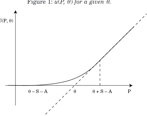
A contractor’s bid maximises his expected profit where the expectation is taken over his competitors’ types and over the cost uncertainty. Let u(P,θ) be the profits to a type θfirm when selected and when the contracted price is P. Under limited liability and in absence of commitment, we have:
u(P, θ) = Es¯max –A, P – (θ + ~ s ) (2)
where Es¯ denotes the expectation taken over the cost uncertainty. This function is continuous and continuously differentiable in P and θ (see Appendix 1). The following notation will be adopted: uk denotes the first derivative with respect to the argument k (k = 1,2), uks denotes the first
derivative with respect to argument k (k = 1,2) and second derivative with respect to argument s (s = 1,2). Figure 1 gives a clearer understanding how profits are modified under limited liability.
The dashed line corresponds to the profit function in absence of limited liability. As limited liability is introduced the function u(P,θ) becomes convex in P (u11 ≥ 0). This means that the risk-neutral contractors behave as
Figure 1: u(P, θ) for a givenθ.
Spulber (1990) shows how the absence of commitment can lead to a pooling equilibrium that destroys the benefits of using an auction. As shown in this lemma, this result cannot be generalised.
Lemma 1 A pooling equilibrium cannot arise unless the minimum level of
profit is zero (A=0).
Proof: Suppose there exists a pooling equilibrium where all contractors submit the same offer, called b, and each wins with probability 1/n. If for some θ, u(P,θ) > 0,then such types would be better-off decreasing slightly their bid (to b –ε) so as to be selected for sure and get a positive expected profit. If for some θ, u(P, θ) < 0, then such types would be better-off increasing their bid not to be selected and get a zero profit instead of a negative expected profit. Thus in equilibrium we can only have u(P,θ) = 0, for all θ. But the level of P
satisfying u(P,θ) = 0 depends on θ. Therefore a pooling equilibrium cannot exist.
When A= 0 bidding b=θ–S (or anything below) can form a pooling equilibrium. In this case, contractors make no profits but cannot improve their situation by bidding more as they would never be selected if they did so.
Proposition 1 In a SPA a monotone, symmetric dominant strategy
equilibrium bidding function, denoted B2(θ), is given by:
u(B2(θ), θ) = 0 (3)
Proof: See Appendix 2. U(P, θ)
In a SPA a bid only sets a lower bound for the price at which they may be contracted. Due to competition, the lowest price they can accept is the one that would generate zero expected profit.
u1(P, θ)
Proposition 2In a FPA, if ——–— is increasing in θ, then there exists a
mono-u(P, θ)
tone, symmetric equilibrium bidding function, B1(θ), that is characterised by
(n – 1)f(θ)
B'1 (θ)u1(B1(θ), θ) – —–——— u(B1(θ), θ) = 0 (4) 1 – F(θ)
and
u(B1(θ–),θ–) = 0 (5)
Proof: see Appendix 3.
A major difference between the first and second price auction is described in the following proposition.
Proposition 3In a SPA there is always a strictly positive probability that the
winning bidder will declare bankruptcy (unless bidders have no liability constraint, i.e. unless A > S). In a FPA, for a sufficiently low cost uncertainty some low cost winning suppliers would never declare bankruptcy.
Proof: see Appendix 4.
To illustrate the latter proposition consider a simple setting where s~ is uniformly distributed and A = 0. In such a case, the SPAequilibrium bidding function is given by:
B2(θ) = θ– S.
In a FPAa monotone, symmetric equilibrium bidding function is given by:
θ∗
S (1 – F(θ*))n–1+
1 – F(t)n–1 dtθ
B1(θ) = θ+ ––––––––––––––––––––––––––––– for θ ≤ θˆ, (6)
θ¯
1 – F(t)n—–12 dtθ
B1(θ) = θ– S + –––––––––––––– for θ ≥ θˆ, (7)
1 – F(θ)n—–12
where θˆ = max{θ, θ*} where θ* satisfies B1(θ*) = θ*. Thus, all types below θ* will always complete the project for no more than the contracted price. For types above θ* limited liability may bind depending on the realisation of the shock. Whether θ* ≥ θ depends on the value of S. As the cost uncertainty increases, more types offer tenders below their highest possible cost.
In the absence of limited liability we know that the sponsor would be indifferent between the FPAand the SPA. Both mechanisms lead to the same expected contracted price and therefore to the same expected cost. This equivalence breaks down under limited liability.
Proposition 4 The FPA leads to a higher expected contracted price than the
SPA.
Proof: see Appendix 5.
The proof shows that the expected price to each type (but typeθ–) in a SPA
is at most equal to their bid in a FPA, and strictly below for some types (on the left of θ–). The intuition is obvious. Risk-lover bidders value more the marginal increase in the rent resulting from slightly increasing their bid than the resulting marginal decrease in the probability of winning. Thus, as they have more control over their rent in a FPA, bidders are less competitive than in a
SPA.
From this proposition one must not conclude that the SPA should be systematically favoured. The contracted price is only one component of the cost of the project. Because the SPAleads to a lower expected contracted price, the likelihood of bankruptcy is higher (in expectation). If the sponsor faces high bankruptcy costs due to delays in completion, or the need of renegotiating, he would be better-off paying a higher price initially.
Finally, the following proposition formally states the implication of limited liability on the bidding behaviour.
Proposition 5Limited liability induces the firms to lower their bids in both
the FPA and the SPA.
This result is obvious since losses are bounded below under limited liability. Thus, it gives all bidders an incentive to bid more aggressively. Still, as we stressed before, the change in the attitude towards risk triggers a countervailing incentive to the preceding one. (An increase in the marginal gain has more value than its associated decrease in the probability of winning.) This trade-off appears clearly when considering the close form solution given as an example. All bidders potentially facing a binding limited liability constraint bid according to:
θ¯
1 – F(t)n—–12 dtθ
B1(θ) = θ– S + –––––––––––––– (8)
1 – F(θ)n—–12
This expression would be the equilibrium bidding function prevailing in absence of limited liability when a bidder has a (lower) cost equal to (θ– S) and
n – 1
faces (less) —–— competitors. The first term reflects the greater competitive-2
ness. Bidders somehow consider the lowest possible cost as their cost. The second reflects the countervailing incentive as it corresponds to the margin a
n – 1
risk neutral bidder would get when facing —–— competitors instead of n – 1. 2
In equilibrium the first incentive dominates the second.
As bidders are more competitive, the contracted price falls when limited liability is introduced. Once again, this is not systematically positive for the sponsor, as it is then more likely that the contractor will not be able to cover the cost ex post. From that perspective, limited liability offers a rationale for the frequency and the size of cost overruns in public contracting.
IV COST MINIMISATION ANALYSIS
Consider now a situation where the sponsor initially designs a procurement contract, i.e. a rule that tells bidders whom will be selected and how much he will be paid as a function of the types they sequentially announce. Assume that the sponsor’s goal is to minimise the (expected) cost of the project. This cost is given by the contracted price whenever it is sufficiently high to guarantee a profit above –A. Otherwise, the sponsor knows that the cost is given by the realisation of (θw+ s) where θw, the winner’s announced type and s are both initially random. For tractability, I consider mechanisms where only the selected firm gets paid.4
Let Θˆ = (θˆ1,…, θˆn) be a vector of types (potentially different from the true
types) and let θˆ–ibe a vector of all types except bidder i’s type. In particular we
have Θˆ = (θˆ–i, θˆi). Let Θ be the vector of true types. Formally, a contract is
defined as a set of functions {xi(Θˆ ), Pi(Θˆ )}i=1,…,n. The function xi(Θˆ ) gives the
probability of selecting firm i. The function Pi gives the price at which firm iis contracted if selected when Θˆ is announced. Most rules will lead contractors to announce a type different from their true type. However, the revelation principle tells us that any rule has an equivalent direct contracting scheme in which contractors find it optimal to reveal their true type. Thus, among all mechanisms we only need to consider those who lead to revelations of true types: {xi(Θ), Pi(Θ)}i=1,…,n. Under incentive compatibility, the project’s cost may
then be written as:
Pi(Θ)–θi+A S
Ti(Θ) =
Pi(Θ)g(~s) ds~ +
(θi + ~ s + C)g(s~) ds~ (9)
–S Pi(Θ)–θi+A
where C includes all bankruptcy costs for which the sponsor is accountable such as costs due to delays in completion.
Given a contracting scheme, the profit to firm i when announcing type θˆi
while others report truthfully is given by:
π(θˆi, θi) = Eθ–ixi(θˆi, θ–i)u(Pi(θˆi, θ–i)θi)]. (10)
Let π(θi,θi)Π(θi). The cost-minimising contract must guarantee
voluntary participation (VP) and incentive compatibility (IC). I will assume that outside opportunities are such that the reservation rents are zero. Thus
VPholds if and only if
Π(θi) ≥0 for all i.
ICholds if and only if:
θi arg max π (θˆi, θi).
θi
From (9) we can see that the cost-minimising contract depends on C. If bankruptcy is particularly costly to the sponsor, he should design a mechanism that limits bankruptcy, i.e. offer a high contracted price.
Proposition 6 If u2(P,θ)is convex in P then the FPA gives the highest expected
contracted price among all efficient mechanisms in which only the selected firm gets paid.
The function u2(P,θ) is convex in P when the distribution function G(.) is concave or linear. It means5that the degree of risk lovingness increases with θi.e. with inefficiency.
The FPAis not a direct mechanism in which it is optimal for bidders to tell their true type. However, as argued above, it has an equivalent incentive compatible direct mechanism that maximises the expected contracted price. The feature of the FPA (and of its equivalent IC mechanism) triggering the result is its deterministic price. In a FPAbidders know exactly what they will be paid if they win: their own bid. Therefore, conditional on winning, uncertainty is eliminated. Because bidders behave as risk-lovers, they are more competitive under more uncertainty. Starting from a FPA, any attempt to raise the expected contracted price by adding uncertainty in the payment will generate lower bids. Due to the risk-loving attitude the decrease in the bids will cause the expected price to fall. Thus, there is no mechanism including a random payment that will generate an expected price higher than the FPA’s expected price.
Unfortunately it is difficult to characterise the cost minimising mechanism for each possible value of C. Still, the following lemma highlights an interesting feature of such contracts.
Lemma 3 The cost minimising contract results from trading off informational
rents and renegotiation costs.
Proof: The sponsor solves:
n
min EΘxi(Θ) Ti(Θ)] (11) {xi(Θ),Pi(Θ)}i=1,…,n i=1
n
subject to (IC), (VP) and xi(Θ) ≤1 with i, xi(Θ) 0, 1. i=1
By adding and substituting the cost, we can rewrite the objective function as:6
n
min EΘxi(Θ) Hi(Θ)] {xi(Θ),Pi(Θ)}i=1,…,n i=1
where
F(θi)
H(Θ) = δ(Pi(Θ), θi) θi + —–— + (1 – δ(Pi(Θ), θi))(C + A+ θi) (12) f(θi)
and where δ(Pi(Θ), θi) is the probability of not facing a binding limited liability
constraint:
5See Lemma 1 in Maskin and Riley (1984).
δ(P, θ) = G(P – θ+ A). (13)
Interestingly, expression (12) tells us that with no commitment there is an upper bound to the informational rents that must be given away to guarantee incentive compatibility. When contracting under asymmetric information, a sponsor must give away some rents to guarantee a truthful revelation of types.
F(θi)
The expression θi + —–— is the so-called virtual costfrom selecting bidder i. f(θi)
It takes into account the informational rents to be left to firm ito guarantee incentive compatibility. Without limited liability these rents would systematically be paid. In the event of bankruptcy giving an amount A
guarantees that the winner makes zero profits whatever he reveals. Thus, under bankruptcy paying Aguarantees IC.
Finally the following results can easily be shown:
1. Setting a minimal acceptable bid in a first price auction would deter efficiency (provided the minimal acceptable bid is above Bi(θ)). As a consequence the sponsor will not always benefit from using such a strategy since inefficient contractors are more likely to face bankruptcy.
2. The mechanisms allowing for payments to all competitors can increase competition (and thus lower the contracted price) if losers must pay a fee. Alternatively, giving a bonus to losers can increase the contracted price. This follows from the risk-loving attitude. To reduce competition the sponsor can provide some insurance to bidders. Lowering the gap between the gain upon losing and the gain upon winning is one way of doing so.
V CONCLUSION
most efficient bidders to never face bankruptcy. Finally, this paper shows that bankruptcy is not always negative as it permits savings on informational rents.
I have taken the view here that bidders differ in their efficiency level. Still, we know that other factors differentiate bidders. It would be interesting to extend this analysis to a model where contractors differ in their level of liabilities. If, as shown, the lowest offer is proposed by the one having the least liabilities, should he still be selected? How can auction rules be designed in such a case to make sure that renegotiation will never be needed?
VI APPENDIX
Appendix 1: Analysing the function u(P, θ).
We have:
– A if P – θ ≤– S – A
u(P, θ) =
û(P,θ) if P – θ – S – A, S – AP – θ if P – θ ≥– S – A,
where
P–θ+A
û(P,θ) = (P – (θ+ s~))g(~s) ds~– A(1 – G(P – θ+ A)) –S
u(P, θ) is continuous in Psince
lim û(P, θ) = – A and lim û(P,θ) = P – θ.
P→θ–S–A P→θ+S–A
Similarly, it is continuous in θsince
lim û(P,θ) = – A and lim û(P,θ) = P – θ.
P→θ+A+S θ→P+A–S
Regarding first partial derivatives we have:
0 if P – θ ≤– S – A
u1(P,θ) =
G(P – θ+ A) if P – θ – S – A, S – A1 if P – θ ≥S – A,
and
0 if P – θ ≤– S – A
u2(P,θ) =
–G(P – θ+ A) if P – θ – S – A, S – A–1 if P – θ ≥S – A.
Appendix 2: Proof of Proposition 1.
The function u(P,θ) is non-decreasing in P and non-increasing in θ. Therefore, the function B2(θ), such that u(B2(θ),θ) = 0, is non-decreasing. Consider now type θ. If she wins when bidding B2(θ) her expected gain will be positive and there is no alternative bid that would make her better off. Indeed, a lower bid would have no effect while a higher bid increases the probability of losing and thus ending up with no revenue. If she loses when bidding B2(θ) it means that the winning bid B* is such that u(B*,θ)≤0. Therefore, undercutting that bid would make her worse-off as the expected gain could be negative. Once again, there is no alternative to B2(θ) that could make her better off.
Appendix 3: Proof of Proposition 2.
Assume there exist a symmetric equilibrium bidding function B1(θ). Assume it is an increasing and continuous function. Because typeθ–never wins it must be the case that u(B1(θ–),θ–) = 0 in equilibrium. Indeed if u(B1(θ–),θ–) > 0, type θ– would be better off lowering its offer slightly so as to win a positive expected gain with a positive probability. If u(B1(θ–),θ–) < 0 then, by continuity
u(B1(θ
–
– ε), θ– – ε) < 0 for εsmall enough. Therefore, type θ– – εwould be better-off bidding B1(θ–) and never win.
If B1(θ) is an equilibrium bidding function, the following must hold:
θ arg max (1 – F(t))n–1u(B 1(t), θ)
t
The first order condition can be written as
u1(B1(t), θ) (n – 1)f(t)
(1 –F(t))
–—–—––— B'1(t) – –—–—–— = 0 at t = θu(B1(t), θ) 1– F(t)
u1(P, θ)
If ———– is increasing in θthen
u(P, θ)
u1(B1(t), θ) (n – 1)f(t) > > ————— B'1(t) – –———— — 0 as t — θ.
u(B1(t), θ) 1– F(t) < <
Therefore the function (1 – F(t))n–1u(B
1(t), θ) reaches a maximum at t = θ as required.
Appendix 4: Proof of Proposition 3. • The second price auction.
The only possibility to have, as a solution, B2(θ) =θarises when u(θ,θ) = 0. Since the expected cost is equal to θ, u(θ,θ) = 0 when the bidder has enough liability to cover any potential loss (i.e. when A ≥ S). If instead A < S, then
u(θ,θ) > 0 and the equilibrium bid is such that b < θ. In that case,
b– (θ+ S) < –Aand the winning bidder will declare bankruptcy with a strictly positive probability.
• The first price auction.
Let A= 0. In a first price auction, the least efficient bidder still proposes a bid such that u(B1(θ
–
),θ–) = 0. Thus, B1(θ
–
) θ–– S, θ–]. The function B1(θ) is such that B1'(θ) < 1 (see expressions (6) and (7) in the text). Thus, moving backwards from θ– it eventually cuts the function (θ+ S). Provided Sis small enough, there exists a unique θ* θ,θ–] such that B1(θ*) = θ* +S and such that B1(θ) >θ+Sfor all θ<θ*. As Aincreases, bids increase as bidders have to cover more losses. Thus, the range of bidders bidding above their highest cost increases.
Appendix 5: Proof of Proposition 47
Let b2(θ) be the expected contracted price paid to type θin a SPA. We will show that b2(θ)≤B1(θ) for all θ and holds strictly for at least one type
b2(θ) <B1(θ). Formally:
θ–
(n– 1)(1 – F(t))n–2f(t)
b2(θ) = B2(t) –—–––––––––—––— dt
(1– F(θ))n–1
θ
Differentiating both sides with respect to θ, we get
(n– 1)f(θ)
b'2(θ) = –—–––— (b2(θ) – B2(θ)). 1– F(θ)
While, for a FPAwe have
(n– 1)f(θ) u(B1(θ), θ)
B'1 (θ) = ––—–––— ––––––––––. 1– F(θ) u1(B1(θ), θ)
Furthermore B1(θ
–
) = B2(θ
–
) = b2(θ
–
). Therefore, showing that B'1(θ) ≤ b'2(θ) whenever B1(θ) = b2(θ) proves that B1(θ) is (almost) everywhere above b2(θ).8 We need to show that
u(B1(θ), θ)
–––––––––– ≤B1(θ) – B2(θ). (14)
u1(B1(θ), θ)
Consider the right and left hand sides as functions of b where b B1(θ). Note that at b= B2(θ) both sides vanish. The derivative of the left-hand side
u11u
(with respect to b) is 1 – ——. The derivative of the right-hand side (with
u12
respect to b) is 1. Because u11≥ 0, and because b = B1(θ) > B2(θ), (14) holds. Thus, b2(θ) ≤ B1(θ) for all θ. Moreover for types facing a potentially binding limited liability constraint u11 > 0. This is the case for all types close enough to θ–. Therefore there exists ε> 0 such that b2(θ
–
– ε) <B1(θ
– – ε).
Appendix 6: Proof of Proposition 5.
The FPAequilibrium bidding function without limited liability, b1(θ) solves:
(n– 1)f(θ)
b'1(θ) = ––—–––— (b1(θ) – θ) 1– F(θ)
and b1(θ
–
) = θ–.
Type θ– always submits a bid –bsuch that u(–b, θ–) = 0. Because limited liability gives a lower bound to u(P, θ–) we have B1(θ
–
) ≤b1(θ
–
). Moreover, for all Pand θ, u1(P,θ) 0, 1] and u(P,θ) ≥P– θ. Thus, for all θsuch that B1(θ) = b1(θ) =
b, we have B'1(θ)≥ b'1(θ). Thus it is true that B1(θ) ≤b1(θ) for all θ.
Appendix 7: Proof of Proposition 6.
I show that if u2(P,θ) is convex in P,then the first price auction is the one giving rise to the higher expected contracted price, among all mechanisms selecting the most efficient firm. The proof consists in showing that the FPAis the mechanism that maximises the bidders revenue. It is done in 5 steps. In what follows I refer to the expected contracted price as the price at which the selected firm is contracted given its type. Finally, the contracted price is the expectation of this price over the winner’s type. At some stage, this proof relies on the necessary and sufficient conditions that guarantee IC. These will be found in Appendix 8.
Step 1: In a FPA the equilibrium bidding function is uniquely defined. Moreover, there does not exist any other efficient mechanism in which the expected contracted price is deterministic. Indeed, it can be shown that if the contracted price is, instead of the winning bid, any monotone transformation of this bid then we will have as an equilibrium bidding function the corresponding monotone transformation of the bidding function. Hence any rules that are monotone transformations of the FPAare equivalent to the FPA.
No monotone transformations are excluded since I restrict attention to efficient rules.
u2(P, θ) = – G(P– θ+ A)
Thus, u2(P, θ) is convex in Pif and only if G(.) is concave. This requirement is not satisfied around P= θ– S – A. However, there is no loss in generalities from considering among all ICmechanisms including a random payment only the ones where Pi(θ) ≥θi – S – A.
Proof: Consider an IC payment scheme such that for some realisations of θi.
Define Pˆi(θ) such that:
Pi(θ) when Pi(θ) ≥θi – S – A, Pˆi(θ) =
————–––––––––——————θi – S – A when Pi(θ) < θi – S – A.
We obviously have ∀θi,π(Pi(θ),θi) =π(Pˆi(θ),θi), since any payment Pi(θ) < θi – S – Agives a rent equal to –Ato the contractor.
Step 3: In any ICmechanism the bidders’ revenue is continuous. This can be shown following Maskin and Riley (1984).
Step 4: The bidders’ revenue is maximised in a FPA.
Let Π1(θi) and Π˜ (θi) be the gains of a type θi firm resulting from a FPAand
any other ICmechanism including a random payment, P˜ (θ), respectively. Let
P1(θi) and EP˜ (θi) denote the expected contracted price of each mechanism.
Note that in a FPA, the contracted price is deterministic and thus equal to the expected contracted price. We have:
θ–
f(θi)
EP˜ (θi) P˜ (θi) ——––——— dθ–i.
(1 – F(θi))n–1
θi
I will show that whenever Π1(θi) = Π˜1'(θi) < Π˜ '(θi). Given that Π1(θ
–
) = Π˜ (θ–) = 0 in any IC mechanism, and given that the gains are continuous, this implies that Π1(θi) > Π˜ (θi) for all θi. (Remember that we are interested in what happens
to the leftof θ–.)
Since contractors act as risk lovers, the rents from a deterministic (FPA) mechanism equal the rents from a random mechanism only if the expected contracted price in the deterministic mechanism is higher. In other words:
Π1(θi) = Π˜ (θi) ⇒P1(θi) > EP˜ (θi)
Recall that the FOCfor ICgives (see Appendix 8):
θ–
Π'(θi) u2(P, θ) f(θ–i) dθ–i. (15)
Since u2(P, θ) is decreasing in P, we have:
P1(θi) > EP˜ (θi) ⇒u2(P1(θi), θi) ≤u2(EP˜ (θi), θi) (16)
If, in addition, u2(P, θ) is convex in P, we have, using Jensen’s inequality:
u2(EP˜ (θi), θi) ≤ EP˜ u2(P˜ (θ), θi) / θi= min
j θj (17)
Given (15), (16) and (17)
P1(θi) > EP˜ (θi) ⇒ Π'1(θi) < Π˜ '(θi)
Step 5: If u(P, θ) is convex in P and given that the bidders’ gain increase with the expected contracted price, we have:
Π1(θi) > Π˜ (θi) ⇒u(P1(θi), θi) ≥u(EP˜ (θi), θi)
⇒ ∀θi, P1(θi) ≥EP˜ (θi)
Thus, at any point the FPA gives a higher expected contracted price to firm i.
Appendix 8: Necessary and Sufficient Conditions for IC.
Lemma 2: A mechanism{xi(Θ), Pi(Θ)}i=1,…,nsatisfies IC if and only if
Π'(θi) = – xi(Θ)δ (Pi(Θ), θi) f(θ–i) dθ–i, (18)
θ–i and
∂
— [xi(r, θ–i)δ (Pi(r, θ–i), θi)] f(θ–i) dθ–i≤0 (19)
∂r
θ–i Proof:
(⇒) By definition, an ICmechanism is such that
θi arg max
r π(r, θi) (20)
where
θ–
π(r, θi) = xi(r, θ–i) u(Pi(r, θ–i), θi) f(θ–i) dθ–i (21)
θ
Using the envelope theorem, we have: ∂π(r, θi)
Π'(θi) = ————
(22)Since u2(P, θ) = –δ(P, θ), where δ(P, θ) is defined by (13), (22) is equivalent to (18).
The second order condition is:
∂2π(r, θ
i)
————
≤0. ∂r2 r=θi
Recall the first order condition:
∂π(r, θi)
——–—
= 0. ∂r r=θi
Differentiating the above with respect to ron both sides, we get:
∂2π(r, θ
i) ∂2π(r, θi)
————
+ ————= 0. ∂r2 r=θi ∂r∂θ
i r=θi Thus, the second order condition can be written as:
∂2π(r, θ
i)
————
≥0, ∂r∂θi r=θi which leads to (19).(⇐) Consider a mechanism such that (18) and (19) hold. Integrating (18) we get:
r θ–
Π(s) – Π(r) = –
xi(t, θ–i) δ(Pi(t, θ–i), t) f(θ–i) dθ–idt (23)s θ
Moreover, by construction, we have:
π(r, s) – Π(r) =
θ–
xi(r, θ–i) u(Pi(r, θ–i), s) – u(Pi(r, θ–i), r)f(θ–i) dθ–i. (24)
θ
We can rewrite (24) as
s θ–
–
xi(r, θi) δ(Pi(r, θi), t) f(θ–i) dθ–idtr θ
Using (19) it is then trivial to show that, given and rand s,
Π(s) – Π(r) ≥ π(r, s) – Π(r)
REFERENCES
ARMSTRONG, MARK, 2000. “Optimal Multi-Object Auctions,’’ The Review of
Economic Studies, Vol. 67, No. 3, pp. 455-481.
MASKIN, ERIC and JOHN RILEY, 1984. “Optimal Auctions with Risk Averse Buyers,’’
Econometrica, Vol. 52, No. 6, pp. 1473-1518.
MATTHEWS, STEVEN, 1987. “Comparing Auctions for Risk Averse Buyers: a Buyer’s Point of View,’’Econometrica, Vol. 55, No. 3, pp. 633-646.
McAFEE, PRESTON R. and JOHN McMILLAN, 1986. “Bidding for Contracts: A Principal-Agent Analysis,’’Rand Journal of Economics, Vol. 17, No. 3, pp. 326-338. MYERSON, ROGER B., 1981. “Optimal Auction Design,’’Mathematics of Operations
Research, Vol. 6, No. 1, pp. 58-73.
RIORDAN, MICHAEL H. and DAVID SAPPINGTON, 1988. “Commitment in Procurement Contracting,’’Scandinavian Journal of Economics, Vol. 90, No. 3, pp. 357-372.
SPIEGEL, YOSSEF, 1996. “The Role of Debt in Procurement Contracts,’’Journal of Economics and Management Strategy, Vol. 5, No. 3, pp. 379-407.
SPULBER, DANIEL F., 1990. “Auctions and Contract Enforcement,’’Journal of Law, Economics, and Organisation, Vol. 2, No. 2, pp. 325-344.
TIROLE, JEAN, 1986. “Procurement and Renegotiation,’’Journal of Political Economy, Vol. 94, No. 2, pp. 235-259.
WAEHRER, KEITH, 1995. “A Model of Auction Contracts with Liquidated Damages,’’