Quasiprobability density diffusion equations for the quantum Brownian motion in a potential

(1)

QUASIPROBABILITY DENSITY

DIFFUSION EQUATIONS

FOR THE

QUANTUM BROWNIAN MOTION

IN A POTENTIAL

BY

BERNARD PATRICK JAMES MULLIGAN, B.A., B.A.I., M.SC.

THESIS SUBMITTED FOR THE DEGREE OF DOCTOR OF PHILOSOPHY (Ph.D.)

TO

DEPARTMENT OF ELECTRONIC AND ELECTRICAL ENGINEERING,

TRINITY COLLEGE DUBLIN

(2)

Declaration

This Thesis is submitted to the University of Dublin, Trinity College, in fulfilment of the requirements for the Degree of Doctor of Philosophy (Ph.D.).

I, the undersigned declare that this work has not previously been submitted to this or any other university and unless otherwise stated is entirely my own work.

Trinity College may lend or copy this Thesis upon request.

Signed:

(3)

Acknowledgments

I would like to thank my supervisor Professor William Coffey for all of his support and encouragement throughout my work. It has been an honour to work with him.

A very special thank you to Professor Yuri Kalmykov and Dr. Sergey Titov without whom this work would not exist.

I would also like to thank Professor Derrick Crothers and Dr. David McCarthy for helpful coversations.

To my family, my friends, thank you for your understanding and patience. To Niamh, with all my love.

(4)

Abstract

Wigner’s [E. P. Wigner, Phys. Rev., 1932, 40, 749] representation of the density operator as a c-number quasiprobablity distribution in phase space allowing quantum mechanical averages involving the density matrix to be calculated as phase space averages just as classical averages originally used by him to obtain quantum mechanical corrections to classical thermodynamic equilibrium i.e. to the Maxwell-Boltzmann distribution so applying to closed quantum systems is extended to open quantum systems comprising a canonical ensemble of Brownian particles in a potential. This is accomplished via an idea of Gross and Lebowitz [E. P. Gross and J. L. Lebowitz, Phys. Rev. 1956, 104, 1528]. They suggested that using Wigner’s representation the connection between classical and quantum collision kernels, (i.e. in classical mechanics the Stosszahlanzatz describing the bath-particle interaction in the open system in the Boltzmann equation for the single particle distribution function) is much more transparent than in the density operator formalism. Moreover the quantum kernel should closely correspond to the classical one. Hence the idea developed in this Thesis that in the quantum Brownian motion the collision term in a quantum master equation in Wigner’s representation should be described by a Kramers– Moyal like expansion truncated at the second term (leading of course in the classical limit to the Fokker-Planck equation) as in the classical Brownian motion. Imposition of the Wigner equilibrium distribution as the stationary solution of this equation (which is akin to the Fokker-Planck equation) in the manner used by Einstein [A. Einstein, in R. H. Fürth, Ed., Investigations on the Theory of the

Brownian Movement, Methuen, London, 1926; reprinted Dover, New York, 1954]

(5)

CHAPTER I

Introductory concepts: reasons for the

development of a theory of quantum

Brownian motion

The classical theory of dissipation based on the Brownian motion (representing the heat bath degrees of freedom) of a particle in a potential is ubiquitous in many areas of applied mathematics, theoretical physics and chemistry, particularly those aspects of nonequilibrium statistical mechanics and fluid mechanics dealing with the nature of metastable states and the rates at which these states decay. (The classical theory is summarized in Chapter II). Typical examples from statistical mechanics are current-voltage characteristics of Josephson junctions, the rate of condensation of a supersaturated vapour, dielectric and Kerr effect relaxation in liquids and nematic liquid crystals, dynamic light scattering, chemical reaction rate theory in condensed phases, superparamagnetic relaxation, polymer dynamics, nuclear fission and fusion and so on [1-4]. All these phenomena in one way or another depend on the nucleation and growth of some characteristic disturbance within a metastable system, e.g., condensation of a saturated vapour is initiated by the formation of a sufficiently large droplet of the liquid. If this droplet is big enough it will be more likely to grow than to dissipate and will bring about condensation of the entire sample [2].

(10)

temperature and at high temperatures a crossover to Johnson-Nyquist noise which is essentially governed by the classical Brownian motion takes place.

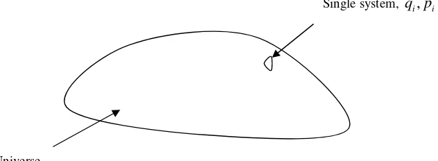
Single system, q p_i, _i

Universe

Figure I.I. The classical dynamics of a collection of N particles where N is of the order of 1023 say, is described by the Liouville equation [1] in the 6N phase space (q,p) where q(t) and p(t) denote the collection of 3N positions and 3N momenta. The Liouville equation describes the time evolution of the phase space density of representative points ρ(q,p) (it is simply a statement of the fact that the representative points are conserved and stream along the constant energy trajectories in phase space) and is

{

}

0

D

H

Dt t

ρ ρ

ρ

∂

≡ + , =

∂

{

}

3

1

N

i i i i i

H H

p q q p

ρ ρ

ρ

=

∂ ∂ ∂ ∂ 

, Η = _ − _

∂ ∂ ∂ ∂

 

∑

where

{

ρ,H

}

is the Poisson bracket, H is the Hamiltonian and the large D’s denote the hydrodynamical derivative. It is a purely dynamical theorem first given by Joseph Liouville in 1838. Boltzmann’s idea (1872) was essentially to replace the entire system of 1023 degrees of freedom by a single (tagged) system of 3 degrees of freedom interchanging energy with the rest of universe or heat bath, i.e. the effect of the remaining 1023−3 degrees of freedom is represented by collisions (this is the Stosszahlansatz) so that for the tagged systemD

Dt

ρ

is no longer zero and the

[image:10.612.166.482.151.267.2]

(11)

attempt to show that whatever the initial state of a gas the Maxwell-Boltzmann distribution must ultimately set in. Later Einstein (1905) used these concepts to great effect to explain the Brownian motion using the Fokker-Planck equation which is a particular form of the Boltzmann equation when the collisions are frequent, but weak. The whole procedure is remarkably well illustrated in the following paragraph from Statistical Physics II, Nonequilibrium Statistical Mechanics, by R. Kubo, M. Toda and N. Hashitsume, 2nd edition Berlin Springer-Verlag, 1991:

“We have emphasized repeatedly that the fundamental logic structure of statistical physics is the derivation of the laws of physics by introducing different stages of coarse graining from microscopic laws. By proceeding a step further, our description is made even cruder than the previous one by partial contraction of information. This contraction is a projection of the object onto a certain cross section of our understanding. Here the problem is to find the appropriate way of describing of the projected process.

For example, the stochastic process called Brownian motion is the projection of the microscopic motion of a colloid particle and all the molecules of the surrounding liquid onto the dimension of the motion of the colloid particle only. Furthermore, if the motion is projected onto the displacement then it becomes a diffusion process of the Brownian particle.

The complete dynamical description of N gaseous molecules confined in a box is made in terms of their position and momentum variables given as functions of time t. If the molecular positions are not observable, then the projected motion is described by the stochastic evolution of the distribution function

1 2

( , ,..., _N, )

f p p p t . The equation governing this evolution is called a master

equation. It should furthermore be possible to discover the probability f r p t₁( , , ) of finding a molecule with momentum p and position r at time t. This is largely contracted information and useful in describing the pas only extremely crudely.

When a colloid particle is much larger and heavier than molecules of the surrounding liquid, the projected process becomes an ideal Brownian motion which is Gaussian and Markovian.”

(12)

macroscopic quantum object. It has been conjectured by Bean and Livingston [5,6] that the magnetization may reverse (so losing the stored information) by quantum tunnelling through the particle internal magnetocrystalline anisotropy barrier as well as by the conventional mechanism of thermally agitated jumping over the barrier [1,7] which is in this context is called Néel relaxation [8]. More precisely by this tunnelling they mean the possibility of transitions of the magnetic moment at absolute zero of temperature from a state of complete alignment to a state of zero overall magnetization, due to the moment tunnelling through the barrier. It is thus immediately apparent that the Brownian motion plays a vital role in information and communications technology as well as in fundamental issues of applied mathematics and theoretical physics such as the existence of quantum tunnelling on a macroscopic scale. One may also remark in the context of macroscopic quantum tunnelling (which is a mesoscale quantum phenomenon) that substantial experimental data on magnetic relaxation now exists [8] at mK temperatures the analysis of which is severely hampered by the lack of an appropriate theory of quantum dissipation which could predict for example the relaxation behaviour as a function of spin size.

(13)

different damping regimes for that quantity may be accurately established [1,11-13]. Wigner’s [14] (c-number) representation of quantum statistical mechanics in terms of phase space distributions (via [15] direct classical analogues of the relevant quantum operators and quantities so that the expectation values of physical variables may be expressed via phase space integration as rapidly converging expansions in Planck’s constant ), is an ideal starting point for the formulation of semiclassical quantum master equations (akin to the Fokker-Planck equation) governing almost classical systems constituting quantum mechanics on the mesoscale.

Now the treatment of the Brownian motion in terms of diffusion (Fokker-Planck) equations by Einstein, Kramers, etc. which is essentially based on a single particle phase space distribution function describing the time evolution of the swarm of moving phase space points and which with the aid of modern computing techniques [1,16] allows one to evaluate various physical parameters ignores quantum effects. If one wishes to include these, however, in a diffusion equation treatment, a difficulty immediately arises, namely one cannot speak, because of the uncertainty principle, [14] of a particle having simultaneously a well defined position and momentum i.e. in the quantum world the concept of a precise phase point has no meaning. In other words it is impossible to ascertain the position of a system in phase space more accurately than to say that it is in a volume of the order of n_{, where}

(14)

impossibility of simultaneously measuring canonical variables) distribution functions have proven [14,18] very useful in quantum mechanical systems as they provide insights into the connection between classical and quantum mechanics allowing one to express quantum mechanical averages in a form which is very similar to that of classical averages. Thus they are ideally suited to the study of the quantum-classical correspondence as is well illustrated by the following remarks of Baker [17] and Stratonovich [19]; Baker: “The large-scale experimental validity of classical mechanics tells us that quantum theory must, in some sense, correspond closely to classical mechanics. We have altered the classical concept of a moving point in phase space to that of a quasi-probability distribution which changes in time. This distribution is imagined to be concentrated about the classical point, so that a crude measurement will be unable to differentiate between the two theories. To ensure this correspondence, we use the statement which actually seems to be given by experiments – on the average, Hamilton’s canonical equations hold”; Stratonovich: “The statistical nature of quantum theory is manifested in the process of physical “measurement.” From this it follows that the “pre-observation” state of a quantum system, which exists before the “measurement” and is independent of it (one can speak of such a state, to be understood in a definite sense), is a statistical state.

In the classical theory the “pre-observation” state of a statistical system is described by distribution functions in a certain space (we denote this space by M). We assume that in the quantum theory such a “pre-observation” state is described by distribution functions in this same “representation” space M, which accordingly has a classical meaning. But owing to the fact that a quantum “measurement” is more complicated than a macroscopic measurement, and is inevitably associated with an integral operation in the representation space, in contrast to the classical situation, negative values of the distribution function are possible at particular points of this space. The “representation distributions” of course do not give an entirely classical interpretation of quantum theory, but they provide a basis for that interpretation of the quantum theory which has maximum closeness to classical ideas and thus has the greatest physical-intuitive meaning.”

(15)

elucidated the role played by tunnelling effects at high temperatures in reaction rate theory [14,18]. The Wigner distribution function was meant to be a reformulation, using the concept of a quasi-probability distribution in phase space, of Schrödinger’s wave mechanics which describes quantum states of functions in configuration space. Thus the Wigner function is of particular use in the statistical mechanics of closed systems (i.e., systems with zero dissipation to the heat bath) as effectively it allows one to consider quantum corrections up to

(

2N

)

O to the classical distribution function, i.e., the quantum-classical correspondence. Hence, Wigner’s formulation originally given for translational motion of a particle provides a basis for mesoscale quantum mechanics. The corresponding phase space representation for spin systems was given by Stratonovich in 1956 [19] who introduced the Wigner quasiprobability density function on the surface of the unit sphere in the phase space of orientations i.e. the polar and azimuthal angles

(

ϑ ϕ,

)

. By way of background we remark that Wigner [14] originally arrived at his quasiprobability density W(x,p) for translational motion of a particle in phase space ( , )x p , which is the quasiprobability representation of the density operator simply by requiring that, the marginal distributions of W(x,p) should yield the correct quantum mechanical probability densities for the position x and momentum p of the particle with Hamiltonian

2

ˆ _ˆ _{/ 2} _{( )}_ˆ

(16)

( , )

W ϑ ϕ is entirely analogous to W(x,p) for the Heisenberg-Weyl group except that certain differences arise because of the angular momentum commutation relations [19]) discovered a linear bijective mapping (cf. Eqs. 1-3 of [19]) between operators on the Hilbert space and functions in representation space. This mapping [22] satisfies a number of physically intuitive properties, covariance and tracing being the two most important, and essentially replaces Moyal’s characteristic function operator. Thus representation space distributions can be determined (see Chapter IV) via this bijective map from the general definition of a representation distribution using the symmetry properties of the underlying group, e.g., the translational Wigner function W x p( , ) is derived [19] by applying the principles of homogeneity and equivalence of directions.

We further remark that extensive computer simulations of Wigner distributions have been carried out by Filinov et al. [23] using molecular dynamics. These simulations are very useful in so far as they provide “experimental” benchmarks for the verification of quantum reaction rate theory and analytic solutions derived from quantum master equations.

Now in the classical Brownian motion a particle constitutes an open

(17)

coefficient in the Fokker-Planck like master equation arising from the truncation of a Kramers-Moyal expansion at the second order term must become a function of the derivatives of the potential as noted in [26]. In the classical theory of the Brownian motion the Kramers-Moyal expansion is simply a differential representation of the Chapman-Kolmogorov integral equation describing the evolution of the transition probability for a Markov process. Truncation at the second term in the Kramers-Moyal expansion is possible for the Gaussian white noise characteristic of the Brownian motion because the higher order statistical moments may be all expressed as powers of the second moment [1]. In assuming a second order truncation of a Kramers-Moyal expansion in the quantum case we are in effect following the remark of Baker above “that quantum theory must in some sense correspond closely to classical mechanics…”

Up to the present, little in the nature of detailed solutions of semiclassical master equations describing quantum Brownian motion in external potentials has appeared in the literature. A notable exception is the Brownian motion of a quantum harmonic oscillator which has been treated by Agarwal [27] and others (see, e.g., refs. [28,29] and references cited therein). However, recently García-Palacios and Zueco [30,31] have proposed an effective approach to the solution of the master equation for the quantum Brownian motion in an anharmonic potential

( )

(18)

basis for the observables [1,16] could be also extended to the quantum regime. This has been successfully accomplished for the first time by the author and his collaborators for the particular case of a periodic cosine potential [26].

Moreover, analytical solutions for various quantum parameters such as escape rates available from quantum rate theory (which has been extensively verified via computer quantum molecular dynamic simulations [23]) have been compared with those obtained from the solution of quantum master equation for this potential. Both solutions essentially agree with each other indicating that our approach via a semiclassical quantum master equation is likely to be fruitful in the future.

(19)

experimental data is hampered by the lack of an adequate theory. See for example [33,34]

In the context of the spin relaxation we should also mention the problem of molecular nanomagnets [35] where the effect of spin size is all-important. In fact one can show experimentally [8] the size effects in the magnetization dynamics and hysteresis loops in going from multi-domain magnetic nanoparticles to molecular clusters. Hence a theoretical method for predicting the magnetization evolution as a function of spin size which would come from extending Stratonovich’s formulation of the Wigner function for spins to include dissipation would be extremely useful particularly to major players in the magnetic recording industry such as Seagate, BASF etc. Finally the Wigner function has extensive practical applications in signal processing, filtering, and engineering (time-frequency analysis), since time and frequency constitute a pair of Fourier-conjugate variables just like the x and p pair of phase space. We mention bioengineering, acoustics, speech analysis, vision processing, turbulence microstructure analysis, radar imaging, seismic data analysis, quantum optics, quantum computing and so on [36].

References

[1] W. T. Coffey, Yu. P. Kalmykov, and J. T. Waldron, The Langevin Equation

(World Scientific, Singapore, 2004), 2nd Ed. [2] J. S. Langer, Ann. Phys. (N.Y.), 54, 258 (1969). [3] P. Hänggi and G. L. Ingold, Chaos, 15, 026105 (2005).

[4] P. Hänggi, P. Talkner, and M. Berkovec, Rev. Mod. Phys. 62, 251 (1990). [5] C. P. Bean and J. D. Livingston, J. App. Phys. 30,120S (1959).

[6] E. M. Chudnovsky, J. Appl. Phys. 73, 6697 (1993). [7] W. F. Brown Jr., Phys. Rev. 130, 1677 (1963). [8] W. Wernsdorfer, Adv. Chem. Phys. 118, 99 (2001).

[9] D. Kohen and D. J. Tannor, Adv. Chem. Phys. 111, 219 (1994).

[10] U.Weiss, Quantum Dissipative Systems (World Scientific, Singapore, 1999). [11] W. T. Coffey, Yu. P. Kalmykov and S. V. Titov, J. Chem. Phys. 120, 9199

(2004).

(20)

[13] Yu. P. Kalmykov, W. T. Coffey, and S. V. Titov, J. Chem. Phys. 124, 024107 (2006).

[14] E. P. Wigner, Phys. Rev. 40, 749 (1932); Z. Phys. Chem. Abt. B 19, 203 (1932).

[15] K. Imre, E. Ozizmir, M. Rosenbaum, and P. Zweifel, J. Math. Phys. 8, 1097 (1967).

[16] H. Risken, The Fokker-Planck Equation, 2nd Edition (Springer, Berlin, 1984; 1989).

[17] G. A. Baker, Phys. Rev. 109, 2198 (1958)

[18] H. Haken, Laser Theory (Springer, Berlin. 1984).

[19] R. L. Stratonovich, Zh. Eksp. Teor. Fiz. 31, 1012 (1956) [Sov. Phys. JETP, 4, 891 (1957)].

[20] S. Heiss and S. Weigert, Phys. Rev. A 63, 012105 (2001). [21] J. E. Moyal, Proc. Cambridge. Philos. Soc. 45, 99 (1949). [22] A. B. Klimov, J. Math. Phys. 43,2202 (2002).

[23] V. S. Filinov, Yu. V. Medvedev, V. L. Kamski, Molec. Phys. 85, 711 (1995).

[24] A. O. Caldeira and A. J. Leggett, Physica A 121, 587 (1983). [25] E. Pollak, Chem. Phys. Lett. 127, 178 (1986).

[26] W. T. Coffey, Yu. P. Kalmykov, S. V. Titov, and B. P. Mulligan, Europhys. Lett. 77 20011, (2007).

[27] G. S. Agarwal, Phys. Rev. A 4, 739 (1971).

[28] J.J. Halliwell and T. Yu, Phys. Rev. D 53, 2012 (1996). [29] R. Karrlein and H. Grabert, Phys. Rev. E 55, 153 (1997).

[30] J. L. García-Palacios and D. Zueco, J. Phys. A 37, 10735 (2004). [31] J. L. García-Palacios, Europhys. Lett. 65, 735 (2004).

[32] H. C. Brinkman, Physica, 22, 29 (1956).

[33] W. Wernsdorfer, E. Bonet Orozco, K. Hasselbach, A. Benoit, D. Mailly, O. Kubo, H. Nakano and B. Barbara, Phys. Rev. Lett. 79, 4014 (1997).

(21)

(22)

(23)

CHAPTER II

Summary of the classical theory of the

Brownian motion

As a background to the development of semiclassical master equations for the quantum Brownian motion it is first necessary to summarize the classical theory. We shall accomplish this first by means of an introductory section outlining in brief the main developments and from that we shall select for a detailed description those parts that are necessary for the development of a quantum theory.

II.I Early developments of the classical Brownian motion

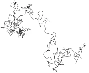
[image:23.612.261.406.389.508.2]

The commonest example of the Brownian motion is the rapid haphazard perpetual motion (Schwankung) of a pollen grain in a colloidal suspension,

Figure II.I. Trajectory of a Brownian particle.

first reported in a meticulous series of observations by the botanist Robert Brown in 1828 [1]. The motion was theoretically explained by Einstein in 1905 [1,2-7] in terms of a discrete time random walk in the diffusion limit of a very large number of microscopic steps with the same variance each taking on average the same

(24)

displacement of a Brownian particle regarded as a sphere in terms of the viscous drag (given by Stokes’ law) imposed by the surroundings, the absolute temperature and the time between successive observations of the displacement of the particle. Einstein envisaged the motion in physical terms as an inescapable consequence of the second law of thermodynamics and as incontrovertible evidence for the existence of atoms as later (1908) verified experimentally by Perrin [1,2]. He used Einstein’s formula in order to determine Avogadro’s number and obtained satisfactory agreement with the accepted value. Einstein’s theory which ignores the inertia of the particle and its subsequent extensions which are listed below effectively allow one to construct a classical theory of dissipative phenomena.

The most significant extensions which are of physical interest [1,2-7] are due to Smoluchowski (1906, who treated the non inertial Brownian motion in an external potential, such as that due to gravity), Langevin (1908, who proceeded from the Newtonian equation of motion of the particle augmented by stochastic terms imposed by the surroundings so rederiving Einstein’s results (in the non inertial limit) and so must be regarded as the founder of the subject of stochastic differential equations; he essentially considered the position and momentum of the particle as random variables), Debye (1913, who considered the non inertial rotational Brownian motion of a rigid rotator in the presence of an applied alternating electric field for the purpose of explaining dielectric relaxation of polar molecules at high frequencies), Ornstein (1917, who included the inertia of the Brownian particle in the formula for the mean square displacement), Klein (1921, who gave a probability density diffusion equation (Klein-Kramers equation) for the evolution of the joint probability density function of the positions and momenta of an assembly of Brownian particles in phase space in the presence of an external potential so that inertial effects could be included exactly), Kramers (1940, who treated noise activated escape over a potential barrier due to the Brownian motion and so was able to predict the influence of solvent friction on the transmission coefficient) [1,2,3,7], Doob (1942, who showed [7] that the proper interpretation of the Langevin equation was as an integral equation leading

(25)

configuration space), and Risken [6] (1983, who developed effective matrix continued fraction algorithms for the exact solution of Brinkman’s recurrence relation using matrix methods based on a Heisenberg-like formulation of the solution of the problem. This is described in Section II.IV below. We summarize Einstein’s theory of the Brownian motion as follows [4].

II.II Einstein’s theory of the Brownian motion

Einstein's theory of the Brownian motion [1,4] is based on the notion that the Brownian particle - a large particle such as a pollen grain suspended in a colloidal suspension executes a discrete time random walk. The walk is due to the very large number of impacts of the surrounding molecules on the Brownian grain. In other words the displacement of the Brownian particle is a sum of random variables, each having arbitrary distributions. We suppose that the density of random walkers in an element x→ +x dx at time t is f. After a discrete time τ has elapsed we consider a neighbouring element of the same size situated at

x′ (τ is supposed so large that the motion of the random walker is independent of its motion at time t±τ yet τ is supposed very small compared to the observation time intervals). We next suppose that the probability of a walker entering from a neighbouring element to x′ is:

(x x, ) ( , )

φ − ′τ =φ ∆τ (2.1)

with:

( , ) ( , )

φ −∆τ =φ ∆τ (2.2)

since we have an unbiased random walker. Summing over all neighbouring elements we then have:

( , ) ( , ) ( , )

f x t τ f x tφ τ d

∞

−∞

+ =

∫

+ ∆ ∆ ∆. (2.3)

(26)

(stosszahlansatz) for the random process must be given i.e. φ(∆,τ) must be specified - here we specify φ by imagining that the random walker moves along the x-axis in such a way that in each step it can move either ∆ to the right or ∆ to the left, the duration of each step being τ , moreover, each individual random walker executes a motion which is independent of the motion of all other walkers in the system. Finally the motion of a random walker at a particular instant is independent of the motion of the random walker at any other instant (the random walker has no memory) that is the motion at time t±τ is statistically independent

of the motion at time t.

Equation (2.3) can however equally well be written by Taylor's theorem as:

( )

0 0

2 ₂

2 0

( , )

! !

2 !

n

n n n

n n

n _n

n n

d

f f

n t n x

f

n x

φ τ

τ

∞

∞ ∞

−∞

= =

∞

=

 

∆ ∆ ∆

 

∂ _ _∂

= _ _

∂ ∂

 

 

∆ _∂ =

∂

∫

∑

(2.4)

by the definition of an average. Moreover, on account of Eq. (2.2) 2 1

0

n+

∆ = . (2.5)

Equation (2.4) which is the simplest form of the Kramers-Moyal [1] expansion is entirely equivalent to the Smoluchowski integral equation. Now let us suppose that ∆ and τ approach zero (extremely small displacements in infinitesimally short times) in such a way that:

2 0 0 lim

2 D

τ∆→→ τ

∆

= (2.6)

and let us further suppose that all terms (τ2

) and (τ4

) and higher vanish in Eq. (2.4) then that equation formally goes over into the diffusion equation:

2 2

f f

D

x x

∂ ∂

=

∂ ∂ (2.7)

where:

0 0 ( , , )

(27)

is the conditional probability that the random walker is in x→ +x dx at time t

given that it was at x0 at time t0. The neglect of the higher order terms in ∆2n as

τ → 0 may be justified as follows. We recall that the probability distribution

φ(∆,τ) of the elementary displacements in time τ arises from the continual buffeting of the random walker by the very large number of impacts by the molecules of the surrounding medium. Thus the resulting displacement ∆ of the walker is the sum of the elementary displacements arising from the molecular collisions (supposed statistically independent) which take place in time τ so that the central limit theorem of probability theory applies. The central limit theorem may be stated as follows [1]; let {ξi} be a sequence of n independent random variables each having arbitrary distributions, then the sum:

1 2 ... n n

ξ ξ ξ

ξ = + + + (2.9)

approaches a normally distributed random variable (in this case ∆) as n → ∞. Furthermore, if ξi has mean zero and variance ξi2 =σi2< ∞ then ξ has mean

zero and variance σ2

where:

2 2

1 1 n

i i n

σ σ

=

∑

. (2.10)

The elementary displacement ∆ is a centred Gaussian random variable thus

2 2

(2 1)!! n

n n

∆ = − ∆ . (2.11)

Equation (2.11) when combined with Eq. (2.4) is the justification for the neglect of the higher order terms in the Kramers-Moyal expansion. The fundamental solution of Eq. (2.7) also called the Green function or propagator is:

[ ]2

0 0

( ) ( ) 4 0 0

0 1 ( , , )

4

x t x t D t t

f x t x t e

D t t

π

− −

−

=

−

(2.12)

which is a centred Gaussian distribution with variance:

[

]

2

0 0

( ) ( ) 2

x t x t D t t

σ = − = − (2.13)

(28)

particle cannot exist. Wiener proved that the realisations (sample paths) [x(t) - x0]

of the Brownian process are almost everywhere continuous but nowhere differentiable. Moreover, Eqs. (2.6) and (2.13) are the same which is an indication of the self-similar nature of the Brownian process. Meaning that any given magnification (subject of course to physical limits such as distances of the order of the mean free path of a molecule) the Brownian motion trajectories appear on average to be the same, that is, the trajectory of a given Brownian particle is a

random fractal [2] (dilation invariant object). The scaling of the steps or segments of the trajectory with magnification defines the fractal dimension which in this case according to the right side of Eq. (2.13) is 2.

To continue, Einstein essentially by considering the Brownian motion of a particle in a potential V(x) and requiring that ultimately the Maxwell-Boltzmann distribution should prevail determined the diffusion coefficient D so finding the famous formula:

2

0 0

2 [ ( )x t x t( )] kT t t

ζ

− = − . (2.14)

In writing Eq. (2.14) it is assumed that the viscous drag on the particle is given by Stokes' Law. ζ is the drag coefficient. Equation (2.14) which connects the mean square fluctuations in the displacement of the Brownian particle with the dissipative coupling to the heat bath is essentially the fluctuation-dissipation theorem. Equation (2.7) in the presence of a potential V(x) which reads:

f f f V

D

t x x ζ x

 

∂ ∂ ∂ ∂

= _ + _

∂ ∂ _ ∂ ∂ _ (2.15)

is called the Smoluchowski differential equation, usually abbreviated to just the Smoluchowski equation. Notice that the second term arises from Stokes’ law essentially as follows because the drift current is J_dr = fv, where

ζ

= F

v and F is the applied force of potential V x( ). The diffusion Eq. (2.15) then follows from the continuity equation f div

t

∂ = −

∂ J where J=Jdr+Jdiff, diff

f D

x

∂ = −

∂

J is the

(29)

potential well will be replaced by the Wigner stationary distribution and the ensuing alterations to the collision term which causes the diffusion coefficient to become a function of the derivatives of the potential will be calculated. In many problems notably in curvilinear coordinates the drift and diffusion coefficients are functions of the coordinates because of the metrics involved.

In 1908 Perrin [1,2] successfully calculated the Avogadro number from observations of the mean square displacement of a Brownian particle so confirming Eq. (2.14).

We remark that Einstein's approach to the Brownian motion is based on statistical assumptions of a general nature, not fixed to a specific model [2]. On the other hand Smoluchowski's investigations which yielded essentially the same results, were published some months later than Einstein's. He considered (in the spirit of Boltzmann) a detailed kinetic model namely collisions of hard spheres as well described by Mazo [2]. Unlike Einstein whose theory is essentially statistical and follows from the central limit theorem, Smoluchowski used the dynamics of the particle motion in a specific dynamic way. The link between the two methods was provided by Langevin in 1908. His idea was [1,2] that a suspended particle in a fluid is acted upon by forces due to the molecules of the solvent. This force can be expressed as a sum of its average value and a fluctuation about this average value. Thus Langevin's starting point is the Newtonian equation:

( ),

d dx

m t

dt dt

υ

ζυ λ υ

+ = = (2.16)

in which the fluctuating force λ(t) has the following properties ( )t 0

λ = (2.17)

1 2 1 2

( ) ( )t t 2kT (t t )

λ λ = ζδ − (2.18)

(30)

( ) (

)

( ) (

)

0 ( ) ( ) ( ) ( )

1 lim

T

F t F t F t F t

F t F t

F t F t d

T

τ τ

′

′→∞

′ = +

=< + >

= +

′

∫

(2.19)

1 2... 2 ( ) ( )... (1 2 2 ) ( ) ( ) ,

i j

n n

k k

t t t

t t

λ λ λ λ λ λ

λ λ

<

≡

=

∑

_∏

(2.20)

where the sum is over all distinct products of expectation value pairs, each of which is formed by selecting n pairs of subscripts from 2n subscripts. For example, when n=2, we have

1 2 3 4 1 2 3 4 1 3 2 4 1 4 2 3

λ λ λ λ = λ λ λ λ + λ λ λ λ + λ λ λ λ

In general, from the theory of permutations and combinations, there will be (2 )!/(2_n n_n!)_{such distinct pairs. We also have for an odd number of observations}

1 2 2 1 1 2 2 1

( ) ( )... ( ) ...

0.

n n

t t t

λ λ λ ₊ ≡ λ λ λ ₊

=

Isserlis’s theorem also known Wick’s theorem allows the truncation of the Kramers-Moyal expansion after the second term as it automatically shows that all the higher order terms are of order of τ2_{and higher (cf the notation following Eq.}

(2.6)). Equation (2.16) (which is the equation of motion of the random variables x

and υ) when averaged over the realizations of the phase path ( , )x v then yields (for convenience setting t₀ =0)

2 2

[ ( ) (0)] 1

t m t

kTm

x t x e

m

ζ

ζ ζ

−

 

− = _ − + _

 

(31)

thermalize exceedingly rapidly. By working in the complete phase space [2] Langevin was also able to find the velocity relaxation.

Einstein’s treatment of the Brownian motion introduces an external force of potential V x( ) only in a virtual sense in order to calculate the diffusion coefficient. The gist of his argument being that the introduction of a potential well causes a Maxwell-Boltzmann distribution to be set up in the well which must then render the collision term in the Fokker-Planck equation zero. The well is necessary in order to have a stationary solution, because for a free Brownian particle no stationary solution exists. The introduction of a virtual force renders Einstein’s analysis more complicated for the beginner than either that of Smoluchowski who includes the well explicitly or Langevin who obtains the constant in his rapidly fluctuating random force by arguing that a Maxwellian distribution of the velocities sets in almost immediately which is true for large particles such as pollen grains.

In general the form of the Fokker-Planck equation for diffusion in one dimension under the influence of an external force is

(1)

2 (2) 2 ( , | )

( , ) ( , | )

f y t x

D y t f y t x

t y

D y t f y t x

y

∂ ∂ _ _

= − _ _

∂ ∂

∂ _ _

+ _ _

∂

(2.22)

where (1)

D is the drift coefficient and (2)

D is the diffusion coefficient. Throughout this Chapter we will specify the distribution by f and we shall distinguish the various distribution functions by quoting their arguments. Clearly Smoluchowski’s differential Eq. (2.15) is a special case of Eq. (2.22).

Since in general we will be dealing with the multivariable form of the Fokker-Planck equation, it is necessary to quote the form of that equation for many dimensions characterized by a set of random variables { } { ,ξ = ξ₁ξ_n}. The multivariable form of the Fokker-Planck equation [6] is with f = f({ }, | { })y t x , { }y denoting a set of realisations of the random variables { }ξ :

(1)

2

(2) , ,

( , )

( , ) ( , ) 1

( , ) ( , ) . 2

i

i i

k l

k l k l

f t

D t f t

t y

D t f t

y y

∂ ∂ _ _

= − _ _

∂ ∂

∂ _ _

+ _ _

∂ ∂

∑

y

y y

(32)

For simplicity, let us suppose that the process is characterised by a state vector y having only two components (y1, y2) (these, for example, could be the realisations

of the position and velocity of a Brownian particle), and so the two variable Fokker-Planck equation written in full is assuming that the 2 dimensional Kramers-Moyal expansion is truncated at the second term,

2 2

(1) (2)

.

1 ,

1 2

i k l

i i k l k l

f

D f D f

t = y y y

∂ ∂ _ _ ∂ _ _

= − _ _+ _ _

∂

∑

∂

∑

∂ ∂ (2.24)

or

2

(1) (1) (2)

1 2 2 1,1

1 2 1

2 2 2

(2) (2) (2)

1,2 2,1 2 2,2

1 2 2 1 2

1 2

1 1 1

.

2 2 2

f

D f D f D f

t y y y

D f D f D f

y y y y y

∂ ∂ _ _ ∂ _ _ ∂ _ _

= − _ _− _ _+ _ _

∂ ∂ ∂ ∂

∂ _ _ ∂ _ _ ∂ _ _

+ _ _+ _ _+ _ _

∂ ∂ ∂ ∂ ∂

(2.25)

In general, (2) (2) 1,2 2,1

D =D so that

(1) (1)

1 2

2 2 2

(2) (2) (2)

1,1 2,2 1,2

2 2

1 2 1 2

1 1

,

2 2

f

D f D f

t y y

D f D f D f

y y y y

∂ ∂ _ _ ∂ _ _

= − _ _− _ _

∂ ∂ ∂

∂ _ _ ∂ _ _ ∂ _ _

+ _ _+ _ _+ _ _

∂ ∂ ∂ ∂

(2.26)

where the various drift and diffusion coefficients are

(1) (2)

,

0 0

lim i, lim i j, ( , 1, 2).

i _t i j _t

y y y

D D i j

t t

∆ → ∆ →

∆ ∆ ∆

= = =

∆ ∆ (2.27)

A particular example of this is the Langevin equation for a free Brownian particle which may be represented as the system describing the random motion of the phase point ( ( ), ( ))x t v t

( ) ,

dx dv t

v v

dt dt m

λ γ

= = − + (2.28)

with

(

)

1 2 1 2

0,

2 .

t

t t m kT t t

λ

λ λ γ δ

( ) =

( ) ( ) = −

This equation may be used to calculate the drift and diffusion coefficients as follows. We have writing the Langevin equation in terms of infinitesimals over a small time ∆t for the first drift coefficient

(1) _lim y1 _lim x

(33)

which follows from the fact that the average of the noise is zero. Now, the change in velocity in a small time ∆t is

1

( )

t t

t

v v t F t dt

m

γ

+∆

′ ′ ∆ ≈ − ∆ +

∫

.

Thus the second drift coefficient D₂(1) is (1) 2 0 lim t v D v t γ ∆ → ∆ = = −

∆ . (2.30)

Likewise, the diffusion coefficients D_1,1(2)( , )x v and D_1,2(2)( , )x v are 2 (2) 1,1 0 2 2 0 ( ) ( , ) lim

( ) lim 0 t t x

D x v

t v t t ∆ → ∆ → ∆ = ∆ ∆ = ∆ = (2.31)

because the numerator is obviously of order

( )

∆t 2. In like manner (2) 1,2 0 0 2 0 ( , ) lim

lim ( ) lim 0 t t t t t t x v

D x v

t

v t v t

F t

v t v dt

m γ ∆ → ∆ → +∆ ∆ → ∆ ∆ = ∆ ∆ ∆ = ∆ ′ ′ = − ∆ + =

∫

(2.32)

because F t( )=0. In order to evaluate the second diffusion coefficient 2

(2) 2,2

0 ( ) ( , ) lim

t v

D x v

t ∆ → ∆ = ∆ (2.33) consider

( )

2 ₂ ₂

( )

2

2 2 ( ) 1 ( ) ( ) . t t t t t t t

v t

v v t F t dt

m

(34)

The first term on the right-hand side of Eq. (2.34) is of order ₍_∆_t₎2_{, the second} term vanishes on averaging, and

( ) ( ) 2 ( )

2

t t t t t t t t

t t t t

F t F t dt dt D t t dt dt

D t

δ

+∆ +∆ +∆ +∆

′ ′′ ′ ′′= ′− ′′ ′ ′′ = ∆

∫ ∫

_(2.35)

(D=γkTm), whence the diffusion coefficient is (2)

2,2( , ) 2 /

D x v = kTγ m. (2.36)

Thus, we obtain

2 2 ( )

f f vf kT f

v

t x γ v m v

 

∂ ∂ ∂ ∂

+ = _ + _

∂ ∂ _ ∂ ∂ _, (2.37)

which is the desired Fokker-Planck equation describing the evolution of the probability distribution of the displacement and velocity of a free Brownian particle in phase space ( ( ), ( ))x t v t . The left hand side of this equation corresponds to the Liouville equation for the single particle distribution function and is the convective derivative which is no longer zero while the right hand side is the Boltzmann collision term arising from the reduction of the many particle distribution function to a single particle one as described earlier. If an external conservative force is introduced nothing new is essentially involved and Eq. (2.37) merely becomes

2 2

1 ( )

f f dV f vf kT f

v

t x m dx v γ v m v

 

∂ ∂ ∂ ∂ ∂

+ − = _ + _

∂ ∂ ∂ _ ∂ ∂ _. (2.38)

(35)

particle superimposed on which is a rapidly fluctuating random force both forces representing the effect of the heat bath on the particle and in the Klein-Kramers equation are represented by the collision term). The continued fraction representation has led to many exact solutions as outlined in [1,6]. In the present context one should also mention that it may be shown (see Appendix II.I) [10] that a generalized Langevin equation, i.e., the equation of motion of a Brownian particle with memory friction is equivalent to the Newtonian equation of motion of a particle moving in a potential V(x)bilinearly coupled to a bath of harmonic oscillators (essentially a string or transmission line attached to the particle which serves as a schematic description of the heat bath) with a high frequency cutoff

ansatz for the spectral density of the bath oscillators.

The particle plus harmonic oscillator heat bath (string), etc. readily lends itself to quantum generalizations. Due to the introduction of the string the number of degrees of freedom becomes essentially infinite. However, this inconvenience is compensated [11,12] by the fact that we now have a conservative dynamical system which can be quantized in the usual manner. The essential ideas go back to Lamb’s [13] attempt to explain radiation damping in classical electrodynamics and Planck’s (1900) inspired treatment of blackbody radiation. One of the most notable quantum generalizations based on such particle-string models is that of Caldeira and Leggett [14] yielding quantum master equations describing nonequilibrium phenomena in phase space leading to generalizations of the Wigner distribution (see Chapter VI).

II.III Klein-Kramers equation and its application to

reaction rate theory

(36)

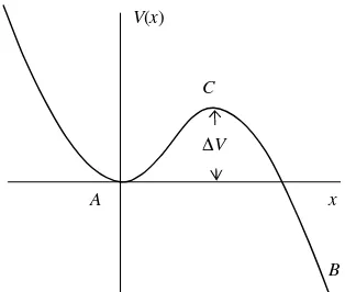
V(x)

B x A

C

∆V

Figure II.II Single well potential function as the simplest example of escape over a barrier. Particles are initially trapped in the well near the point A by a high potential barrier at the point C. They very rapidly thermalise in the well. Due to thermal agitation however very few may attain enough energy to escape over the barrier into region B whence they never return.

For simplicity the particles of mass m are supposed having crossed the barrier never to return. This leads to the following formula [4] for the rate constant (formally defined as the current or flux of particles at the barrier divided by the population of the particles in the well)

( ) 1

2

V V

A

kT kT

A

V x

e e

m

ν

π

∆ ∆

− ′′ −

Γ = = (2.39)

which was originally proposed by Arrhenius from analysis of experimental data. An elementary derivation of Eq. (2.39) is given in Chapter V. Equation (2.39) however has the flaw that the prefactor νA is simply the frequency of oscillation

in the well (the attempt frequency) and is thus entirely independent of the dissipative coupling of the particles in the well to the surrounding heat bath. Thus escape of particles may occur in the absence of fluctuations so violating the fluctuation dissipation theorem. Another way of stating this is that in the transition state or equilibrium theory the Maxwell-Boltzmann distribution which prevails in the depths of the well is assumed to hold everywhere. This is not true near the top of the barrier due to the leaking of particles over the barrier. The problem of incorporating nonequilibrium effects which is essentially a boundary layer problem was first attacked by Kramers [16]. In 1940 he suggested that Eq.(2.39) should be replaced by:

[image:36.612.248.405.68.201.2]

(37)

where A is a (transmission) factor describing the dissipative coupling of the bath to the well. The aim is to calculate the transmission factor A as a function of the coupling. Kramers accomplished this by generalizing, as we have just seen, Einstein's theory of the Brownian motion to yield the complete phase space description, (i.e. Eq. (2.38) above), of the Brownian motion which is then used as a model of the dissipative coupling. The Klein-Kramers equation applies to systems, which (ignoring the bath coordinates) have a separable additive Hamiltonian of the form:

2 1

( ) 2

H = mx +V x (2.41)

and is entirely equivalent to the Langevin equation: ( )

V

mx x t

x

ζ ∂ λ

+ + =

∂

(2.42)

provided λ(t) is Gaussian white noise. Kramers obtained asymptotic solutions for the prefactor A from Eq. (2.38) in two limiting cases. The first is called very low damping which may be explained as follows: Here he proceeded by rewriting Eq. (2.38) in angle-action variables (or equivalently angle-energy variables). Then he supposed that the energy trajectories form essentially closed (apart from a critical energy curve known as the separatrix on which the particle may escape) loops so that they do not differ significantly from those of the undamped librational motion in the well with energy equal to the barrier or saddle energy ∆V . Next since the motion is very lightly damped the loss of energy in one cycle of the motion is very small i.e. the energy is a slow variable (it is almost conserved) while the angle or phase is a fast variable. Thus eliminating the phase by averaging along an energy trajectory over the fast phase variable yields a diffusion equation in the energy. The solution of this energy diffusion equation ultimately leads to the escape rate for very low damping (VLD). We have:

( ) ( ) 2

V

c kT

A

V c

A kT

J E e

m kT

J E e kT

ζ ν

ω γ

π

∆ −

Γ = =

(2.43)

where

m

(38)

so that

( _c)

A=γJ E

where γJ E( _c)is the energy loss per cycle of the almost periodic motion along the barrier (saddle) energy trajectory, Ec = ∆V and J(Ec) is the action evaluated at the barrier energy. The approximation νAJ(Ec) ∼ Ec = ∆V may be used to render Eq. (2.43) in an even simpler form. Equation (2.43) which unlike Eq. (2.39) precludes escape without coupling to the bath holds if in Eq. (2.40) A1 that is when:

( _c)

J E E kT

γ = ∆ . (2.44)

Thus the energy loss per cycle of the almost periodic motion of the saddle energy trajectory is much less than the thermal energy. Kramers also obtained an asymptotic solution for the escape rate for very high damping (VHD) namely

E kT

∆ :

( ) ( ) V

A C _kT

V x V x

e

ζ

∆ −

′′ ′′

Γ = (2.45)

which is often written:

2

V A C_e kT

ω ω πγ

∆ −

(2.46) so that:

C

A ω

γ

= . (2.47)

Thus unlike the transition state theory escape is precluded for very small

or very large coupling to the bath. Moreover at a certain critical coupling where (∆E ∼ kT) a transition in the escape rate from ζ to inverse ζ dependence occurs. This region is much more difficult to treat as no small perturbation parameter exists [1,17] (see our discussion at the end of this Section). Equation (2.46) which does not include inertial effects may be determined entirely either from the Smoluchowski differential equation (for the distribution function in configuration space which neglects inertia) or from the very high friction limit of the Kramers asymptotic solution of the Klein-Kramers equation for the escape rate for ∆E >

kT. The asymptotic solution is valid in the so called intermediate to high damping

(39)

2 2 1

2 4 2

V

A kT

C C

e

ω γ γ

π ω ω

∆ −

 

Γ =  + − 

 

 

(2.48) where intermediate damping is defined as the γ = 0 value of Eq. (2.48) which corresponds to the TST result where the transmission factor is unity.

Equation (2.48) includes inertial effects but is not valid for very small damping. In its derivation which requires linearization of the Langevin equation about the saddle point (in this one dimensional case a simple maximum) one assumes that the thermal distribution prevails almost to the top of the well. This is not true for small damping because the nonequilibrium region extends into the depths of the well far beyond the saddle point region where the Langevin equation may be linearized. It goes over into the VHD damping result for large γ. The Kramers calculation (which explains the riddle of escape in the absence of fluctuations, associated with the transition state theory) applies to mechanical systems with separable and additive Hamiltonians of the form of Eq.(2.41). It was generalized to systems of n degrees of freedom and non-separable Hamiltonians by Langer [1,17,18] in the IHD case he obtained:

det det

V

A kT

C E

e E

λ

∆ − +

Γ = . (2.49)

Thus the escape rate is expressed in terms of the Hessians of the saddle and well energies and the (unstable) positive eigenvalue λ+_{, of the set of noiseless}

(40)

compared to all the other eigenvalues. This has been accomplished for a large variety of systems by Risken [6] and Coffey et al. [1] in the context of dielectric and magnetic relaxation. λ1 may also be calculated by averaging the Langevin

equation over its realisations as described by Coffey et al. [1] and solving the resulting hierarchy of equations for the statistical averages by matrix continued fraction methods.

Kramers was however, unable to find asymptotic solutions valid in the so called Kramers turnover region, where the energy loss per cycle of a particle having the saddle point energy is of the order of the thermal energy. Here the coupling between the Liouville and dissipative terms in the Klein–Kramers equation enters so that one may no longer ignore the Liouville term as was done in his solution for the very low damping regime. (The Liouville term vanishes when averaged over the fast variable in the VLD case by the principle of the conservation of density in phase). This problem, named the Kramers turnover problem, was solved nearly 50 years later by Mel’nikov and Meshkov [20]. They gave an integral formula namely

( 2 )

( ) 1/ 4

IHD 2

1

exp ln 1

2 1/ 4

C I E

kT d

e

γ

λ λ

π λ

∞

− +

−∞

   

Γ = _  −  _Γ

+

 



∫



(41)

the absolute lower limit of validity of the IHD solution as a function of friction). Thus they postulate from heuristic reasoning, essentially appealing to continuity that a formula valid in all damping regimes may be given by simply multiplying the general IHD result by the depopulation factor, i.e. Eq. (2.50). Besides their use in reaction rate theory these asymptotic solutions which hold of course only when the barrier height is significantly greater than the thermal energy are also very useful as benchmark solutions in the numerical calculation of escape reaction rates i.e. the smallest non vanishing eigenvalue for matrix continued fraction solution of the Klein-Kramers equation. They also lend themselves to quantum generalizations which we now briefly summarize as they will be used in Chapter VI.

First Mel’nikov [11,12] extended the depopulation factor method to take into account quantum effects in a semiclassical ad hoc way by simply inserting the quantum mechanical transmission factor for a parabolic barrier [22] into the classical integral equation for the energy distribution function yielded by the Wiener-Hopf method in the Kramers turnover region. On solving for the energy distribution function and proceeding to the VLD limit he was able to obtain an integral formula for the VLD quantum Kramers rate which at high temperatures reduces to the classical VLD result. Moreover, he gave explicit expressions for the quantum VLD rate for cubic and cosine potentials (for details see Section 3.4 of [11]). These results simplify if the potential well is assumed to be very wide so that the noise can be treated as classical; see Eqs. (15) and (16) of [12] here it is possible to give a simple analytic formula for the VLD quantum Kramers rate; see Eq. (16) of Ref. [11].

(42)

Pollak [23,24] using the string-particle model. Mel’nikov’s idea is also likely to be of use in obtaining the VLD result even if an explicit quantum Fokker-Planck equation in phase space is known due to the difficulty in transforming such an equation into energy/angle variables (when the diffusion coefficient becomes a function of the derivatives of the potential) in order to obtain an energy diffusion equation in the manner of Kramers. However, the ad hoc insertion of the parabolic barrier transmission factor requires rigorous justification. Following Mel’nikov and Meshkov [20], Grabert [25] and Pollak et al. [26] presented a complete solution of the classical Kramers turnover problem and have shown that the Mel’nikov and Meshkov universal formula can be obtained without their ad hoc interpolation between the weak and strong damping regimes. In the semiclassical limit, the latter theory was extended to the quantum regime by Rips and Pollak [27] where a review and comparison of the various approaches is given. We remark that comprehensive reviews of applications and developments of Kramers’ reaction rate theory have been given by Hänggi et al. [28], Mel’nikov [11], Coffey et al. [17], and Pollak and Talkner [29]. These review articles provide one with a detailed theoretical description of reaction rate theory, a variety of examples of its application, relevant references, and even indicate future open problems to be tackled.

Quasiprobability density diffusion equations for the quantum Brownian motion in a potential