Evaluating Sentiment Analysis Evaluation: A Case Study in Securities Trading

Evaluating Sentiment Analysis Evaluation: A Case Study in Securities

Trading

Siavash Kazemian Shunan Zhao

Department of Computer Science University of Toronto

{kazemian,szhao,gpenn}@cs.toronto.edu

Gerald Penn

Abstract

There are numerous studies suggesting that published news stories have an im-portant effect on the direction of the stock market, its volatility, the volume of trades, and the value of individual stocks men-tioned in the news. There is even some published research suggesting that auto-mated sentiment analysis of news doc-uments, quarterly reports, blogs and/or Twitter data can be productively used as part of a trading strategy. This paper presents just such a family of trading strategies, and then uses this application to re-examine some of the tacit assumptions behind how sentiment analyzers are gen-erally evaluated, in spite of the contexts of their application. This discrepancy comes at a cost.

1 Introduction

Amidst the vast amount of user-generated and professionally-produced textual data, analysts from different fields are turning to the natural lan-guage processing community to sift through these large corpora and make sense of them. Interna-tional collaborative projects such as the Digging into Data Challenge (2012) or the Big Data Con-ference sponsored by the Marketing Science In-stitute (2012) are some recent examples of these initiatives.

The proliferation of opinion-rich text on the World Wide Web, which includes anything from product reviews to political blog posts, led to the growth of sentiment analysis as a research field more than a decade ago. The market need to quan-tify opinions expressed in social media and the blogosphere has provided a great opportunity for sentiment analysis technology to make an impact in many sectors, including the financial industry,

in which interest in automatically detecting news sentiment in order to inform trading strategies ex-tends back at least 10 years. In this case, senti-ment takes on a slightly different meaning; posi-tive sentiment is not the emotional and subjecposi-tive use of laudatory language. Rather, a news article that contains positive sentiment is optimistic about the future financial prospects of a company.

Zhang and Skiena (2010) have shown that news sentiment can effectively inform simple market neutral trading algorithms, producing a maximum yearly return of around 30%, and even more when using sentiment from blogs and Twitter data. They did so, however, without an appropriate baseline, making it very difficult to appreciate the signif-icance of this number. Using a very standard sentiment analyzer, we are able to garner annual-ized returns over twice that percentage (70.1%), and in a manner that highlights some of the bet-ter design decisions that Zhang and Skiena (2010) made, viz., their decision to use raw SVM scores rather than discrete positive or negative senti-ment classes, and their decision to go long (resp., short) in the n best- (worst-) ranking securities rather than to treat all positive (negative) securi-ties equally. We trade based upon the raw SVM score itself, rather than its relative rank within a basket of other securities, and tune a threshold for that score that determines whether to go long, neu-tral or short. We sample our stocks for both train-ing and evaluation with and withoutsurvivor bias, the tendency for long positions in stocks that are publicly traded as of the date of the experiment to pay better using historical trading data than long positions in random stocks sampled on the trad-ing days themselves. Most of the evaluations of sentiment-based trading either unwittingly adopt this bias, or do not need to address it because their returns are computed over historical periods so brief. We also provide appropriate trading base-lines as well as Sharpe ratios to attempt to

tify the relative risk inherent to our experimen-tal strategies. As tacitly assumed by most of the work on this subject, our trading strategy is not portfolio-limited, and our returns are calculated on a percentage basis with theoretical, commission-free trades.

Our motivation for undertaking this study has been to reappraise the evaluation standards for sentiment analyzers. It is not at all uncommon within the sentiment analysis community to eval-uate a sentiment analyzer with a variety of classi-fication accuracy or hypothesis testing scores such as F-measures, kappas or Krippendorff alphas de-rived from human-subject annotations, even when more extensional measures are available. In secu-rities trading, this would of course include actual market returns from historical data. With Holly-wood films, another popular domain for automatic sentiment analysis, one might refer to box-office returns or the number of award nominations that a film receives rather than to its star-rankings on review websites where pile-on and confirmation biases are widely known to be rampant. Are the opinions of human judges, paid or unpaid, a suf-ficient proxy for the business cases that actually drive the demand for sentiment analyzers?

We regret to report that they are not. We have even found a particular modification to our stan-dard financial sentiment analyzer that, when eval-uated against an evaluation test set sampled from the same pool of human-subject annotations as the analyzer’s training data, returns significantly poorer performance, but when evaluated against actual market returns, yields significantly better performance. This should worry researchers who rely on classification accuracies and hypothesis tests relative to human-subject data, because the improvements that they report, whether based on better feature selection or different pattern recog-nition algorithms, may in fact not be improve-ments at all.

The good news, however, is that, based upon our experience within this particular domain, training on human-subject annotations and then tuning on more extensional data, in cases where the latter are less abundant, seems to suffice for bringing the evaluation back to reality. A likely machine-learning explanation for this is that whenever two unbiased estimators are pitted against each other, they often result in an improved combined perfor-mance because each acts as a regularizer against

the other. If true, this merely attests to the relative independence of task-based and human-annotated knowledge sources. A more HCI-oriented view would argue that direct human-subject annotations are highly problematic unless the annotations have been elicited in manner that isecologically valid. When human subjects are paid to annotate quar-terly reports or business news, they are paid re-gardless of the quality of their annotations, the quality of their training, or even their degree of comprehension of what they are supposed to be doing. When human subjects post film reviews on web-sites, they are participating in a cultural activ-ity in which the qualactiv-ity of the film under consider-ation is only one factor. These sources of annota-tion have not been properly controlled.

2 Related Work in Financial Sentiment Analysis

Studies confirming the relationship between me-dia and market performance date back to at least Niederhoffer (1971), who looked at NY Times headlines and determined that large market changes were more likely following world events than on random days. Conversely, Tetlock (2007) looked at media pessimism and concluded that high media pessimism predicts downward prices. Tetlock (2007) also developed a trading strategy, achieving modest annualized returns of 7.3%. En-gle and Ng (1993) looked at the effects of news on volatility, showing that bad news introduces more volatility than good news. Chan (2003) claimed that prices are slow to reflect bad news and stocks with news exhibit momentum. Antweiler and Frank (2004) showed that there is a significant, but negative correlation between the number of mes-sages on financial discussion boards about a stock and its returns, but that this trend is economically insignificant. Aside from Tetlock (2007), none of this work evaluated the effectiveness of an actual sentiment-based trading strategy.

There is, of course, a great deal of work on automated sentiment analysis as well; see Pang and Lee (2008) for a survey. More recent de-velopments that are germane to our work include the use of different information retrieval weighting schemes (Paltoglou and Thelwall, 2010) and the utilization of Latent Dirichlet Allocation (LDA) in a joint sentiment/topic framework (Lin and He, 2009).

sentiment of financial documents without actually using those results in trading strategies (Koppel and Shtrimberg, 2004; Ahmad et al., 2006; Fu et al., 2008; O’Hare et al., 2009; Devitt and Ahmad, 2007; Drury and Almeida, 2011). As to the rela-tionship between sentiment and stock price, Das and Chen (2007) performed sentiment analysis on discussion board posts. Using this analysis, they built a “sentiment index” that computed the time-varying sentiment of the 24 stocks in the Morgan Stanley High-Tech Index (MSH), and tracked how well their index followed the aggregate price of the MSH itself. Their sentiment analyzer was based upon a voting algorithm, although they also dis-cussed a vector distance algorithm that performed better. Their baseline, the Rainbow algorithm, also came within 1 percentage point of their reported accuracy. This is one of the very few studies that has evaluated sentiment analysis itself (as opposed to a sentiment-based trading strategy) against mar-ket returns (versus gold-standard sentiment anno-tations). Das and Chen (2007) focused exclusively on discussion board messages and their evaluation was limited to the stocks on the MSH, whereas we focus on Reuters newswire and evaluate over a wide range of NYSE-listed stocks and market capitalization levels.

Butler and Keselj (2009) try to determine sen-timent from corporate annual reports using both character n-gram profiles and readability scores. They also developed a sentiment-based trading strategy with high returns, but do not report how the strategy works or how they computed the re-turns, making the results difficult to compare to ours. Basing a trading strategy upon annual re-ports also calls into question the frequency with which the trading strategy could be exercised.

The work that is most similar to ours is that of Zhang and Skiena (2010). They look at both financial blog posts and financial news, forming a market-neutral trading strategy whereby each day, companies are ranked by their reported sen-timent. The strategy then goes long and short on equal numbers of positive- and negative-sentiment stocks, respectively. They conduct their trading evaluation over the period from 2005 to 2009, and report a yearly return of roughly 30% when us-ing news data, and yearly returns of up to 80% when they use Twitter and blog data. Further-more, they trade based upon sentiment ranking rather than pure sentiment analysis, i.e., instead of

trading based on the raw sentiment score of the document, they first rank the documents and trade based on this relative ranking.

Zhang and Skiena (2010) compare their strat-egy to two strategies which they term Worst-sentiment Strategy and Random-selection Strat-egy. The Worst-sentiment Strategy trades the op-posite of their strategy, going short on positive sen-timent stocks and going long on negative senti-ment stocks. The Random-selection Strategy ran-domly picks stocks to go long and short in. As trading strategies, these baselines set a very low standard. Our evaluation compares our strategy to standard trading benchmarks such as momentum trading and holding the S&P, as well as to oracle trading strategies over the same trading days.

3 Method and Materials

3.1 News Data

Our dataset consists of a combination of two col-lections ofReutersnews documents. The first was obtained for a roughly evenly weighted collec-tion of 22 small-, mid- and large-cap companies, randomly sampled from the list of all companies traded on the NYSE as of 10th_{March, 1997. The}

second was obtained for a collection of 20 com-panies randomly sampled from those comcom-panies that were publicly traded in March, 1997 and still listed on 10th _{March, 2013. For both collections}

of companies, we collected every chronologically third Reuters news document about them from the period March, 1997 to March, 2013. The news articles prior to 10th _{March, 2005 were used as}

training data, and the news articles on or after 10th

March, 2005 were reserved as testing data. We chose to split the dataset at a fixed date rather than randomly in order not to incorporate future news into the classifier through lexical choice.

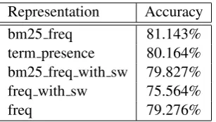
Representation Accuracy bm25 freq 81.143% term presence 80.164% bm25 freq with sw 79.827% freq with sw 75.564%

freq 79.276%

Table 1: Average 10-fold cross validation ac-curacy of the sentiment classifier using different term-frequency weighting schemes. The same folds were used in all feature sets.

3.2 Sentiment Analysis and Intrinsic Evaluation

For each selected document, we first filter out all punctuation characters and the most common 429 stop words. Our sentiment analyzer is a support-vector machine with a linear kernel function im-plemented using SVMlight_{(Joachims, 1999). We}

have experimented with raw term frequencies, bi-nary term-presence features, and term frequen-cies weighted by the BM25 scheme, which had the most resilience in the study of information-retrieval weighting schemes for sentiment analysis by Paltoglou and Thelwall (2010). We performed 10 fold cross-validation on the training data, con-structing our folds so that each contains an approx-imately equal number of negative and positive ex-amples. This ensures that we do not accidentally bias a fold.

Pang et al. (2002) use word presence features with no stop list, instead excluding all words with frequencies of 3 or less. Pang et al. (2002) nor-malize their word presence feature vectors, rather than term weighting with an IR-based scheme like BM25, which also involves a normalization step. Pang et al. (2002) also use an SVM with a linear kernel on their features, but they train and com-pute sentiment values on film reviews rather than financial texts, and their human judges also clas-sified the training films on a scale from 1 to 5, whereas ours used a scale that can be viewed as being from -1 to 1, with specific qualitative inter-pretations assigned to each number. Antweiler and Frank (2004) use SVMs with a polynomial kernel (of unstated degree) to train on word frequencies relative to a three-valued classification, but they only count frequencies for the 1000 words with the highest mutual information scores relative to the classification labels. Butler and Keselj (2009) also use an SVM trained upon a very different set

of features, and with a polynomial kernel of degree 3.

As a sanity check, we measured the accuracy of our sentiment analyzer on film reviews by training and evaluating on Pang and Lee’s (Pang and Lee, 2004) film reviews dataset, which contains 1000 positively and 1000 negatively labelled reviews. Pang and Lee conveniently labelled the folds that they used when they ran their experiments. Using these same folds, we obtain an average accuracy of 86.85%, which is comparable to Pang and Lee’s 86.4% score for subjectivity extraction.

Table 1 shows the performance of SVM with BM25 weighting on our Reuters evaluation set versus several baselines. All baselines are iden-tical except for the term weighting schemes used, and whether stop words were removed. As can be observed, SVM-BM25 has the highest sentiment classification accuracy: 80.164% on average over the 10 folds. This compares favourably with pre-vious reports of 70.3% average accuracy over 10 folds on financial news documents (Koppel and Shtrimberg, 2004). We will nevertheless adhere to normalized term presence for now, in order to stay close to Pang and Lee’s (Pang and Lee, 2004) implementation.

4 Task-based Evaluation

In our second evaluation protocol, we evaluate the accuracy of the sentiment analyzer by embedding the analyzer inside a simple trading strategy, and then trading with it.

Our trading strategy is simple: going long when the classifier reports positive sentiment in a news article about a company, and short when the classi-fier reports negative sentiment. In section 4.1, we use the discrete polarity returned by the classifier to decide whether go long/abstain/short a stock. In section 4.2 we instead use the raw SVM score that reports the distance of the current document from the classifier’s decision boundary.

In section 4.3, we hold the trading strategy con-stant, and instead vary the document representa-tion features in the underlying sentiment analyzer. Here, we measure both market return and classifier accuracy to determine whether they agree.

In all three experiments, we compare the per-position returns of trading strategies with the fol-lowing four standards, where the number of days for which a position is held remains constant:

of the stockhdays ago, wherehis the hold-ing period. Then, it goes long forh days if the previous price is lower than the current price. It goes short otherwise.

2. The S&P strategy simply goes long on the

S&P 500for the holding period. This strat-egy completely ignores the stock in question and the news about it.

3. The oracle S&P strategy computes the value of theS&P 500indexhdays into the future. If the future value is greater than the current day’s value, then it goes long on theS&P 500

index. Otherwise, it goes short.

4. The oracle strategy computes the value of the stock h days into the future. If the future value is greater than the current day’s value, then it goes long on the stock. Otherwise, it goes short.

The oracle and oracle S&P strategies are included as toplines to determine how close the experimen-tal strategies come to ones with perfect knowledge of the future. “Market-trained” is the same as “ex-perimental” at test time, but trains the sentiment analyzer on the market return of the stock in ques-tion forhdays following a training article’s publi-cation, rather than the article’s annotation.

4.1 Experiment One: Utilizing Sentiment Labels in the Trading Strategy

Given a news document for a publicly traded com-pany, the trading agent first computes the senti-ment class of the docusenti-ment. If the sentisenti-ment is positive, the agent goes long on the stock on the date the news is released. If the sentiment is neg-ative, it goes short. All trades are made based on the adjusted closing price on this date. We evalu-ate the performance of this strevalu-ategy using four dif-ferent holding periods: 30, 5, 3, and 1 day(s).

The returns and Sharpe ratios are presented in Table 2 for the four different holding periods and the five different trading strategies. The Sharpe ratio can be viewed as a return to risk ratio. A high Sharpe ratio indicates good return for rela-tively low risk. The Sharpe ratio is calculated as follows:

S = pE[Ra−Rb]

var(Ra−Rb),

whereRais the return of a single asset andRbis

the return of a risk-free asset, such as a 10-year U.S. Treasury note.

Strategy Period Return S. Ratio

Experimental

30 days -0.037% -0.002 5 days 0.763% 0.094 3 days 0.742% 0.100 1 day 0.716% 0.108

Momentum

30 days 1.176% 0.066 5 days 0.366% 0.045 3 days 0.713% 0.096 1 day 0.017% -0.002

S&P

30 days 0.318% 0.059 5 days -0.038% -0.016 3 days -0.035% -0.017 1 day 0.046% 0.036

Oracle S&P

30 days 3.765% 0.959 5 days 1.617% 0.974 3 days 1.390% 0.949 1 day 0.860% 0.909

Oracle

30 days 11.680% 0.874 5 days 5.143% 0.809 3 days 4.524% 0.761 1 day 3.542% 0.630

Market-trained

30 days 0.286% 0.016 5 days 0.447% 0.054 3 days 0.358% 0.048 1 day 0.533% 0.080 Table 2: Returns and Sharpe ratios for the Experi-mental, baseline and topline trading strategies over 30, 5, 3, and 1 day(s) holding periods.

Figure 1: Percent returns for 1 day holding period versus market capitalization of the traded stocks.

which we are familiar, based on the details that they publish. One may note, however, that the re-turns from the experimental strategy have slightly higher Sharpe ratios than either of the baselines.

One may also note that using a sentiment ana-lyzer mostly beats training directly on market data, which to an extent vindicates the use of sentiment annotation as a separate component.

Figure 1 shows the market capitalizations of the companies for each individual trade plotted against the percent return for the 1 day holding pe-riod. The correlation between the two variables is not significant. The graphs for the other holding periods are similar.

Figure 2 shows the percent change in share value plotted against the raw SVM score for the different holding periods. We can see a weak cor-relation between the two. For the 30 days, 5 days, 3 days, and 1 day holding periods, the correlations are 0.017, 0.16, 0.16, and 0.16, respectively. The line of best fit is shown.

This prompts us to conduct our next experiment.

4.2 Experiment Two: Utilizing SVM scores in Trading Strategy

4.2.1 Variable Single Threshold

Previously, we would label a document as positive (negative) if the score is above (below) 0, because 0 is the decision boundary. However, 0 might not be the best threshold for providing high returns. To examine this hypothesis, we took the evaluation dataset, i.e. the dataset with news articles dated on or after March 10, 2005, and divided it into two folds where each fold has an equal number of

doc-uments with positive and negative sentiment. We used the first fold to determine an optimal thresh-old valueθand trade using the data from the sec-ond fold and that threshold. For every news article, if the SVM score for that article is above (below)

θ, then we go long (short) on the appropriate stock on the day the article was released. A separate theta was determined for each holding period. We variedθfrom−1to1in increments of0.1.

Using this method, we were able to obtain much higher returns. In order of 30, 5, 3, and 1 day hold-ing periods, the returns were 0.057%, 1.107%, 1.238%, and 0.745%. This is a large improvement over the previous returns, as they are average per-position figures.1

4.2.2 Safety Zones

For every news item classified, SVM outputs a score. For a binary SVM with a linear kernel func-tion f, given some feature vector x,f(x) can be viewed as the signed distance of x from the de-cision boundary (Boser et al., 1992). It is then possibly justified to interpret raw SVM scores as degrees to which an article is positive or negative. As in the previous section, we separate the eval-uation set into the same two folds, only now we use two thresholds,θ > ζ. We will go long when the SVM score is aboveθ, abstain when the SVM score is betweenθ andζ, and go short when the SVM score is belowζ. This is a strict generaliza-tion of the above experiment, in whichζ =θ.

For convenience, we will assume in this section thatζ =−θ, leaving us again with one parameter to estimate. We again varyθ from0 to1 in in-crements of0.1. Figure 3 shows the returns as a function ofθfor each holding period on the devel-opment dataset. If we increased the upper bound onθto be greater than1, then there would be too few trading examples (less than 10) to reliably cal-culate the Sharpe ratio. Using this method with

θ= 1, we were able to obtain even higher returns: 3.843%, 1.851%, 1.691, and 2.251% for the 30, 5, 3, and 1 day holding periods, versus 0.057%, 1.107%, 1.238%, and 0.745% in the second task-based experiment.

4.3 Experiment Three: Feature Selection

Let us now hold the trading strategy fixed (at the final one, with safety zones) and turn to the un-derlying sentiment analyzer. With a good trading

Figure 2: Percent change of trade returns plotted against SVM values for the 1, 3, 5, and 30 day holding periods in Exp. 1. Graphs are cropped to zoom in.

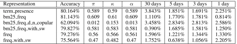
Representation Accuracy π κ α 30 days 5 days 3 days 1 day term presence 80.164% 0.589 0.59 0.589 3.843% 1.851% 1.691% 2.251% bm25 freq 81.143% 0.609 0.61 0.609 1.110% 1.770% 1.781% 0.814% bm25 freq d n copular 62.094% 0.012 0.153 0.013 3.458% 2.834% 2.813% 2.586% bm25 freq with sw 79.827% 0.581 0.583 0.581 0.390% 1.685% 1.581% 1.250%

freq 79.276% 0.56 0.566 0.561 1.596% 1.221% 1.344% 1.330%

freq with sw 75.564% 0.47 0.482 0.47 1.752% 0.638% 1.056% 2.205%

Table 3: Sentiment classification accuracy (average 10-fold cross-validation), Scott’sπ, Krippendorff’s

α, Cohen’sκand trade returns of different feature sets and term frequency weighting schemes in Exp. 3. The same folds were used for the different representations. The non-annualized returns are presented in columns 3-6.

strategy in place, it is clearly possible to vary some aspect of the sentiment analyzer in order to deter-mine its best setting in this context. Is classifier ac-curacy a suitable proxy for this? Indeed, we may hope that classifier accuracy will be more portable to other possible tasks, but then it must at least correlate well with task-based performance.

We tried another feature representation for doc-uments. In addition to evaluating those attempted earlier, we now hypothesize that the passive voice may be useful to emphasize in our representations, as the existential passive can be used to evade re-sponsibility. So we add to the BM25 weighted vector the counts of word tokens ending in “n” or “d” as well as the total count of every conjugated form of the copular verb: “be”, “is”, “am”, “are”, “were”, “was”, and “been”. These three features are superficial indicators of the passive voice.

Table 3 presents the returns obtained from these 6 feature representations. The feature set with BM25-weighted term frequencies plus the number of copulars and tokens ending in “n”, “d” (bm25 freq d n copular) yields higher returns than any other representation attempted on the 5, 3, and 1 day holding periods, and the second-highest on the 30 days holding period, But it has the worst classification accuracy by far: a full 18 percentage points below term presence. This is a very compelling illustration of how misleading an intrinsic evaluation can be. Other agreement mea-sures likewise point in the opposite direction.

5 Conclusion

In this paper, we examined the application of senti-ment analysis in stock trading strategies. We built a binary sentiment classifier that achieves high ac-curacy when tested on movie data and financial news data from Reuters. In three task-based ex-periments, we evaluated the usefulness of senti-ment analysis in simple trading strategies.

Al-though high annual returns can be achieved by simply utilizing sentiment labels in a trading strat-egy, they can be improved by incorporating the output of the SVM’s decision function. We have observed that classification accuracy alone is not always an accurate predictor of task-based perfor-mance. This calls into question the benefit of using intrinsic sentiment classification accuracy, partic-ularly when the relative cost of a task-based eval-uation may be comparably low. We have also de-termined that training on human-annotated senti-ment does in fact perform better than training on market returns themselves. So sentiment analysis is an important component, but it must be tuned against task data.

As for future work, we plan to explore other ways of deriving sentiment labels for supervised training. It would be interesting to infer the senti-ment of published news from stock price fluctua-tions instead of the reverse. Given that many fac-tors that affect stock price fluctuations and further considering the drift that is present in stock prices as a result of bad published news (Chan, 2003), this mode of inference is not simple and requires careful consideration and design.

Furthermore, we would like to study how senti-ment is defined in the financial world. In particu-lar, we want to examine the relationship between the precise definition of news sentiment and trad-ing strategy returns. This study has used a rather general definition of news sentiment. We are in-terested in exploring if there is a more precise def-inition that can improve trading performance.

References

Khurshid Ahmad, David Cheng, and Yousif Almas. 2006. Multi-lingual sentiment analysis of financial

news streams. In Proceedings of the 1st

Interna-tional Conference on Grid in Finance.

Werner Antweiler and Murray Z Frank. 2004. Is all that talk just noise? the information content of

inter-net stock message boards. The Journal of Finance,

59(3):1259–1294.

Bernhard E. Boser, Isabelle M. Guyon, and

Vladimir N. Vapnik. 1992. A training

algo-rithm for optimal margin classifiers. InProceedings of the fifth annual workshop on Computational learning theory, COLT ’92, pages 144–152, New York, NY, USA. ACM.

Matthew Butler and Vlado Keselj. 2009. Finan-cial forecasting using character n-gram analysis and readability scores of annual reports. InProceedings of Canadian AI’2009, Kelowna, BC, Canada, May. Wesley S. Chan. 2003. Stock price reaction to news

and no-news: Drift and reversal after headlines.

Journal of Financial Economics, 70(2):223–260. Sanjiv R. Das and Mike Y. Chen. 2007. Yahoo! for

amazon: Sentiment extraction from small talk on the web. Management Science, 53(9):1375–1388. Joseph Davies-Gavin, Clarence Lee, and Lingling

Zhang. 2012. Conference summary. InMarketing

Science Institute Conference on Big Data, Decem-ber.

Ann Devitt and Khurshid Ahmad. 2007. Sentiment polarity identification in financial news: A cohesion-based approach. InProceedings of the ACL. Brett Drury and J. J. Almeida. 2011. Identification

of fine grained feature based event and sentiment

phrases from business news stories. InProceedings

of the International Conference on Web Intelligence, Mining and Semantics, WIMS ’11, pages 27:1–27:7, New York, NY, USA. ACM.

Robert F. Engle and Victor K. Ng. 1993. Measuring

and testing the impact of news on volatility. The

Journal of Finance, 48(5):1749–1778.

Tak-Chung Fu, Ka ki Lee, Donahue C. M. Sze, Fu-Lai Chung, Chak man Ng, and Chak man Ng. 2008. Discovering the correlation between stock time se-ries and financial news. In Web Intelligence, pages 880–883.

Thorsten Joachims. 1999. Making large-scale svm learning practical. advances in kernel methods-support vector learning, b. sch¨olkopf and c. burges and a. smola.

Moshe Koppel and Itai Shtrimberg. 2004. Good news

or bad news? let the market decide. InAAAI Spring

Symposium on Exploring Attitude and Affect in Text, pages 86–88. Press.

Chenghua Lin and Yulan He. 2009. Joint

senti-ment/topic model for sentiment analysis. In

Pro-ceedings of the 18th ACM conference on Informa-tion and knowledge management, CIKM ’09, pages 375–384, New York, NY, USA. ACM.

Victor Niederhoffer. 1971. The analysis of world events and stock prices. Journal of Business, pages 193–219.

Neil O’Hare, Michael Davy, Adam Bermingham, Paul Ferguson, P´araic Sheridan, Cathal Gurrin, and Alan F. Smeaton. 2009. Topic-dependent

senti-ment analysis of financial blogs. In Proceedings

of the 1st international CIKM workshop on Topic-sentiment analysis for mass opinion measurement. Georgios Paltoglou and Mike Thelwall. 2010. A study

of information retrieval weighting schemes for

sen-timent analysis. InProceedings of the ACL, pages

1386–1395. Association for Computational Linguis-tics.

Bo Pang and Lillian Lee. 2004. A sentimental educa-tion: Sentiment analysis using subjectivity

summa-rization based on minimum cuts. InProceedings of

the ACL, pages 271–278.

Bo Pang and Lillian Lee. 2008. Opinion mining and sentiment analysis. Foundations and trends in infor-mation retrieval, 2(1-2):1–135.

Bo Pang, Lillian Lee, and Shivakumar Vaithyanathan. 2002. Thumbs up?: sentiment classification using

machine learning techniques. InProceedings of the

ACL-02 conference on Empirical methods in natu-ral language processing - Volume 10, EMNLP ’02, pages 79–86, Stroudsburg, PA, USA. Association for Computational Linguistics.

Paul C. Tetlock. 2007. Giving content to investor

sen-timent: The role of media in the stock market. The

Journal of Finance, 62(3):1139–1168.

Christa Williford, Charles Henry, and Amy Friedlan-der. 2012. One culture: Computationally inten-sive research in the humanities and social sciences. Technical report, Council on Library and Informa-tion Resources, June.