Sensitivity of the damping controlled fluidelastic instability threshold to mass ratio, pitch ratio and Reynolds number in normal triangular arrays

School of Engineering

Department of Mechanical & Manufacturing Engineering

Sensitivity of the damping controlled

fluidelastic instability threshold to

mass ratio, pitch ratio and Reynolds

number in normal triangular arrays.

Beatriz de Pedro & Craig Meskell

Published in Nuclear Engineering and Design (2018)

CITATION INFORMATION:

Sensitivity of the damping controlled fluidelastic

instability threshold to mass ratio, pitch ratio and

Reynolds number in normal triangular arrays.

Beatriz de Pedro Palomara, Craig Meskellb,∗

a_{School of Engineering, Univeristy of Oviedo, Spain} b_{School of Engineering, Trinity College Dublin, Ireland}

Abstract

Sensitivity of the damping controlled fluidelastic instability threshold of

nor-mal triangular tube arrays has been investigated through a theoretical-CFD

hybrid methodology without the need for experimental data. The

quasi-unsteady model with a theoretical model of the memory function was used

to predict the critical velocity with the static fluid force coefficients obtained

from steady RANS simulations. Five normal triangular tube arrays with

pitch to diameter ratios of 1.25, 1.30, 1.32, 1.375 and 1.44 were investigated.

Pressure on the tube surface for theP/d= 1.32 array, predicted by the CFD,

was compared with empirical measurements from the literature. Force

coef-ficients obtained with the validated numerical model, were used to predict

stability thresholds for the P/d = 1.25 and P/d = 1.375 tube arrays and

the results were compared with previously published experimental critical

velocities. The validated theoretical-CFD hybrid methodology was used to

analyze and quantify the critical velocity specific dependence on three

pa-rameters: mass ratio, Reynolds number and pitch ratio. As expected, the

pitch ratio has the most effect on the critical velocity. It was found that

increased Reynolds number increases the stability threshold over the whole

range of mass-damping parameters, but mass ratio has only a very minor

effect, and this is confined to high mass-damping values.

Keywords:

Fluidelastic Instability, Heat exchanger, Tube arrays

1. Introduction

Flow-induced vibration (FIV) can be a major problem in large heat

ex-changers leading to shut down or even decommissioning. While turbulent

buffeting and the associated wear represents a limit on the long term

in-tegrity of these assemblies, fluidelastic instability (FEI) can lead to failure in

the short term. As a result, FEI represents a limitation on the operational

parameters of the unit. One particular mechanism of FEI, so-called damping

controlled instability, can occur when a single flexible tube is subjected to

cross flow, even within an otherwise rigid array. It is this mechanism which

is the focus of the current study. An exhaustive review of the literature

on damping controlled fluidelastic instability in normal triangular tube

ar-rays is beyond the scope of this paper, but a comprehensive introduction to

FEI in tube arrays can be found in, for example, Chapter 5 of Paidoussis

et al. (2011) and a review of available models for specifically for damping

controlled fluidelastic instability is given by Price (1995). Broadly speaking,

any of the available models require some experimental input or tuning. For

example, even one of the most theoretical the framework proposed by Lever

when it is extended to predict damping controlled instability (Yetisir and

Weaver, 1993a) an empirical delay function is necessary.

Previous models of FEI and schemes for collapsing experimental data

sets of critical velocity have assumed that the Reynolds number and mass

ratio have no effect on levels of critical velocity. However, there is some

experimental evidence that this may not be the case (Mewes and Stockmeier,

1991). Price (2001) in his discussion of the applicability of the Connors

equation noted that a complete model of FEI should also include a Reynolds

number dependency. Mahon and Meskell (2012) have shown that a Reynolds

number dependency is necessary to achieve agreement between the Connors

type equation and the quasi-steady model. Harran (2014) pointed out the

influence of the mass ratio, in an asymptotic approach for the theoretical

situation of an undamped structure.

The viability of using CFD, computational fluid dynamics, to obtain

non-dimensional force coefficients, as well as other previously empirically

deter-mined quantities, and then introduce them into a theoretical framework to

obtain stability thresholds, has been investigated by several authors.

Has-san et al. (2010) investigated pitch to diameter ratio and Reynolds Number

effects on critical velocity for in-line tube arrays by obtaining coefficients

for a unsteady the semi-empirical model framework of Chen (1983) from

numerical simulations. Khalifa et al. (2013) investigated the interaction

between tube vibrations and flow perturbations at lower reduced velocities

and Reynolds numbers, coupling numerical predictions of the phase lag and

the semi-analytical wavy wall model (Lever and Weaver, 1986; Yetisir and

developed a model to account for temporal variations in the flow separation

for in-line arrays. These types of study offer an interesting alternative to

experimental testing which is limited for physical and economical reasons,

allowing more extensive investigation of parameter effects in the reduced

critical velocity.

This study will use steady CFD calculations of the fluid force coefficients

on a displaced tube within an array to predict the critical velocity, using

the quasi-unsteady model of Granger and Paidoussis (1996) with the

mem-ory function obtained from the wake model proposed by Meskell (2009).

The approach is applied to single-phase flow, but it is conceivable that the

approach could be adapted to phase flow if an appropriate model of

two-phase damping is adopted, and an equivalent parameter to Reynolds number

could be well defined.

Gillen and Meskell (2009) completed a preliminary study using a

simi-lar approach, demonstrating that the scheme was promising. However, that

study had significant flaws: the simulations suffered from flow instability in

the far wake; only two geometries were simulated; and the range of

parame-ters investigated was small. It is important to note that the objective in this

study is not to advance a method of determining the critical velocity per se.

Rather, the goal of the current study is to investigate the dependence of the

critical velocity on mass ratio and Reynolds number.

2. Methodology

Consider a single flexible tube in an otherwise rigid array. It will be

(i.e. perpendicular to the mean bulk flow) and that the structure can be

represented by a single degree of freedom model. This excludes the possibility

of (coupled mode) stiffness controlled instability. In addition, streamwise

instability is not possible.

The fluidelastic force E that a tube in an array is subjected to, can be

expressed by the governing equation of motion

msy¨+csy˙+ksy=Fy(¨y,y, y, U˙ 0) (1)

The quantities ms, cs and ks are the structural mass, damping and stiffness

respectively. The effects of both turbulent buffeting and vortex shedding have

been omitted as it is assumed that they do not change the stability behaviour

of this model. This superposition effectively assumes that the dependency

of the fluid force on the tube displacement is linear at low amplitudes (i.e.

at the onset of instability). Note that if the post-stable behaviour was of

interest (i.e. the limit cycle amplitude) then a more sophisticated approach

would be needed, but as the focus of this study is the onset of instability,

the simplification of a linear relationship with displacement is acceptable.

Meskell and Fitzpatrick (2003) demonstrated that the fluidelastic stiffness

and damping were cubic in displacement and tube velocity respectively. As

a result, the onset of dynamic instability will be governed by the linear

pa-rameters. This is generally true in non-linear system dynamics, for example

see Chapter 3 of Virgin (2000). Furthermore, these assumptions are widely

made in models of fluidelastic instability. For example, Price and Paidoussis

(1984) and Lever and Weaver (1986) implicitly assume that the only fluid

force is due to tube displacement.

var-ious models have been developed. One such model used the quasi-steady

approach (Price and Paidoussis, 1984), which assumes the force on the

oscil-lating tube at any moment in time is equal to the force it would experience

at that static displacement, but subject to a time lag. This model was later

improved upon by Granger and Paidoussis (1996), by replacing the time lag

as a function spread over time. In this quasi-unsteady model, the

relation-ship between the instantaneous fluid forces and the static lift and drag force

coefficients is

Fy(t) = −

1 2ρd

2_LC

My¨+

1 2ρU

2_Ld(dCL

dy h∗y−Cdy˙) (2)

The terms of this equation consist of tube diameter, d, and length, L; the

fluid densityρ; freestream velocity,U; and the mass, lift and drag coefficients

(CM, CL and CD respectively). The tube displacement y is convolved with

the delay function h. The drag, which would normally only be considered

for forces in the x direction is included due to the quasi-steady assumption

which rotates the fluid force system to be aligned with the instantaneous

apparent flow direction. It is worth noting that the strict requirement for

the application of the quasi-steady assumption as stated by Van Oudheusden

(1995) is that it is possible to ”define a steady situation (in which the

struc-ture is in rest with regard to some suitably chosen reference frame) which

is aerodynamically equivalent to the unsteady situation”. But this cannot

be met in a tube array because of the proximity of the neighbouring tubes.

Nonetheless, it is clear that there should be a positive damping associated

with the fluid which will be modified by flow, and so the quasi-steady

as-sumption is included as an imperfect model of this stabilizing effect as its

The convolution integral can be represented as

h∗y=

Z τ

0

h(τ −τ0)y(τ0)dτ0 (3)

with h representing the memory function

h(τ) = dΦ

dτ (4)

where τ = tU_d is the non-dimensional time. The convolution can also be

thought of as a low pass filter and so that any response to any vortex

shed-ding and most turbulent excitation will be attenuated, further justifying

the assumption in equation 1 to ignore these excitation mechanisms. The

transient evolution of this memory function, which is essential for damping

controlled FEI, is determined by the function Φ. This transient function

converges monotonically towards 1 as τ approaches infinity (Granger and

Paidoussis, 1996). Without loss of generality, it can be represented this as a

series of decaying exponentials:

Φ = 1−

N

X

i=1

αie−βiτ

!

H(τ) (5)

Granger and Paidoussis (1996) quantified the parameters αi and βi by

fit-ting the model response to experimental data of critical velocity in a normal

triangular array subject to cross flow. Li and Mureithi (2016) have

quan-tified these parameters for a parallel triangular array, also by comparison

with experimental data, although the main focus of their study was the

de-velopment of a frequency domain formulation, equivalent to a Theodorsen

function. However,Paidoussis et al. (2011) pointed out that using

for empirical data, largely negating the benefit of a model. Meskell (2009)

has proposed a wake model to predict theoretically the values of α1 and β1

for a first order model, i.e. N = 1 in eqn. 5 .

This wake model approach assumes that the memory function is the

nor-malized instantaneous bound circulation on the tube. The wake is modeled

as a discretized vortex sheet. The convection of the shed vorticity is assessed

in an idealized velocity field based only on the enforcement of the

continu-ity equation along the gap between tubes. The resulting one dimensional

relationship for the temporal variation in lift force on the tube is an

integro-differential equation which cannot be solved analytically (Saffman, 1992),

but a first order model of the memory function is quantified by numerical

quadrature. The non-dimensional values obtained in that study and used

here are α1 = 1.0 and β1 = 0.1572.

In principle, this approach can be applied to any tube array pattern,

but to date, the particular wake model has only been developed for normal

triangular arrays. Although it is currently limited to a normal triangular

array, this approach has the advantage that no additional experimental data

is needed and it does not produce the large overshoots at low non-dimensional

time observed in both the fitted memory function of Granger and Paidoussis

(1996) or Li and Mureithi (2016).

As the underlying mechanism which gives rises to the memory function is

a convection effect, it will have only a weak dependency on Reynolds number

if at all. Mahon and Meskell (2013) measured experimentally the time delay

associated with the Price and Paidoussis (1984) quasi-steady model (which is

quasi-unsteady model used here). They found that the time delay was independent

of both Reynolds number and reduced velocity. The effect of Reynolds

num-ber will be embedded in the variation of the lift and drag coefficients, which

are obtained from steady simulations.

At the critical flow velocity net damping in the coupled system is zero.

Practically, the value of the critical flow velocity is obtained by transforming

the equation of motion eqn.2 into the Laplace domain by assuming a

sinu-soidal free response. The resulting characteristic equation is a polynomial,

the coefficients of which depend on both the structural parameters and the

fluid force parameters, including the flow velocity. The solution of this scalar

polynomial is a complex number, with the real part being the frequency of

vibration and the imaginary part being the damping. Some manipulation

yields yields a quartic polynomial in the critical velocity:

4

X

i=1

piUci = 0 (6)

in which pi = pi(ζ0, mr, CD,dC_dyL, α1, β1). Derivation of these expressions is

tedious, but straight forward. Details can be found in Appendix 1 of Meskell

(2009). The only required input data for the model to predict critical

veloc-ities are the structural properties ζ0 (the damping ratio), and mr (the mass

ratio), along with the static fluid force coefficients CD and dC_dyL. Previously

these force coefficients have been obtained via experimental testing.

How-ever, in this study these static fluid force coefficients will be determined from

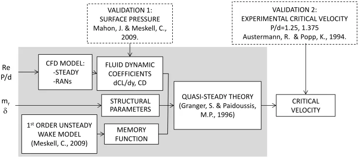
2.1. Summary of methodology.

The overall hybrid theoretical-CFD model to predict the critical velocity

is shown schematically in Fig. 1. For a given tube array pitch ratio a series of

steady RANS simulations are conducted to yield the lift and drag coefficients

at a range of static tube displacements. The onset flow velocity is changed

to vary the Reynolds number. The resulting static fluid force coefficients are

then combined with the structural parameters (mass ratio,mrand structural

damping, δ) in the quasi-steady theory proposed by Granger and Paidoussis

(1996) using the memory function obtained from the wake model (Meskell,

2009). By solving eqn 6, the resulting hybrid model yields a prediction of the

critical velocity which can be assessed for across a range of Reynolds number,

mass ratio and pitch ratio, as presented in Section 4.

3. Validation of the hybrid theoretical-CFD model

The aim of the study is to investigate the variation of the critical velocity

with mass ratio, pitch ratio and Reynolds number. In order to demonstrate

that the hybrid model described in Fig. 1 is appropriate for such an

inves-tigation, the approach has been validated at two levels. Firstly, the steady

CFD simulation of flow through a deformed array have been compared to

experimental surface pressure data. This also facilitated the choice of

tur-bulence model. The second level of validation was achieved by comparing

the predicted critical velocity from the entire model to experimental data in

the literature. Five normal triangular tube array geometries were considered

in this study. In all cases the tube diameter was d=38 mm. Pitch ratios

of 1.25, 1.32 and 1.375 were chosen to allow for comparison and validation

of the model, as P/d= 1.32 was used by Mahon and Meskell (2009) in their

surface pressure measurements, while P/d=1.25 and P/d=1.375 were used

by Austermann and Popp (1995) in their experimental estimation of critical

velocity.

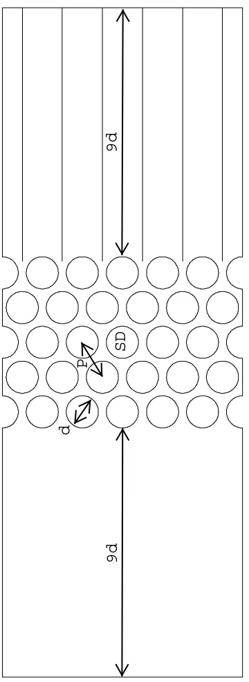
3.1. Computational domain and scheme

The commercial CFD package ANSYS Fluent 12.1 was used to perform

steady simulations, using a 2D double precision Reynolds Averaged

Navier-Stokes solver, considering a displaced tube in the central position of the third

row only. A convergence criteria for residuals of 10−5_{was necessary to achieve}

a stable solution. Figure 2 shows a typical velocity magnitude contour plot

obtained in these simulations. The flow field is affected by the top and

bottom boundaries. This is most obvious in the wake, but flow retardation

can also be seen in front of the half tubes. However, in the center of the

array the flow field is unaffected.

In order to minimize the effect of the arbitrary constant pressure outlet

condition the downstream outlet should be distant from the zone of interest

in the array (26th ITTC Specialist Committee on CFD, 2011). However,

this space behind the array allows wake oscillations downstream of the

ar-ray. Note that these oscillations are probably physical rather than numerical

artifacts, but they would not be present in a deep array typical of a steam

generator. A similar problem was reported by Hassan et al. (2010). In this

study the oscillations were suppressed using full-slip guide vans, with

negligi-ble thickness which were placed behind each tube gap of the last row. These

down-stream of the array shown schematically in Figure 3. The inflow condition

is a Dirichlet boundary condition on the velocity field, while the outlet is a

Dirichlet condition on the pressure field. The top and bottom boundaries

are slip walls (i.e. zero shear stress, zero normal velocity). Within the array

200 elements of equal circumferential length were used around each tube.

The cells adjacent to the surface have an initial thickness of 0.06 mm and a

growth factor of 1.15 until the 13th_{row of the mesh. This allows the mesh to}

be deformed to achieve a static displacement, rather than regenerated, and

it provides a maximum y+ _{value of the order of 1 for all simulations. The}

near wall mesh is structured quadrilateral, while away from the surface of

the tubes the mesh is unstructured triangular. A detail of the mesh between

the tubes can be seen in figure 4 . The density and design of the mesh was

arrived at after a mesh dependency study. Further details of the

computa-tional scheme, the mesh and mesh independence can be found in a related

study de Pedro et al. (2016).

3.2. Comparison with experimental surface pressure data

In order to choose an appropriate turbulence model, several simulations

were conducted for theP/d= 1.32 array, so that the simulated data could be

compared directly to the experimental data Mahon and Meskell (2009). This

pitch ratio does not exhibit bi-stable flow, and so it is straight forward to

com-pare the experimental surface pressure. The flow conditions and displacement

range of the experimental data were matched (2.1×104 _{≤ Re ≤1.1×10}5_;

0 ≤ ∆y ≤ 0.1d). Three models were compared: k − RNG with

non-equilibrium wall function, SST and k−ω. The predicted surface pressure

P∗ = Pθ−Pθ|max Pθ|max−Pθ|min

(7)

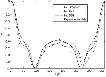
Figure 5 shows the pressure coefficient (Eqn. 7) on the central tube

ob-tained with the three turbulence models and the experimental measurements

of Mahon and Meskell (2009), for the particular case of Re= 2.1×104 _and

∆y = 0. Note that θ is defined as zero at the front of the tube. It is clear,

that both the SST and the k −ω models predict substantial asymmetry in

the pressure distribution. This is particularly acute in the regions around

θ = 90◦ and θ = 270◦, which are the top and bottom of the tubes. Due to the surface normal direction, these regions will contribute most to the

transverse (lift) force and so are of particular concern in estimating the fluid

force coefficients for damping controlled fluidelastic instability. This general

behaviour was found for all velocities and displacements examined. While it

is true that asymmetric flow fields have been observed in tube arrays (Keogh

and Meskell, 2015; Mahon and Meskell, 2009, e.g.), it is unlikely that the

asymmetry observed in fig. 5 is due to bistable flow for two reasons. Firstly,

the numerical model included no-slip guide vanes immediately downstream

of the tube array specifically to suppress the large wake structures that give

rise to bistable flow inside an array. Secondly, and more importantly, the

asymmetric behaviour was observed at all pitch ratios including the lower

values. In normal triangular arrays, Mahon and Meskell (2009) did not

ob-serve any bistable flow behaviour for p/d = 1.32 as shown in fig. 5, but did

for P/d= 1.58. This would suggest that the asymmetry in the pressure field

is an artifact of the numerical scheme.

func-tions wall treatment was chosen. This is a pragmatic decision, based on the

comparison with experimental pressure data. It is not meant as a

recom-mendation for best practice in modelling flow in tube arrays, nor is it argued

that this turbulence model is inherently superior. In fact, it is well known

that the k− performs poorly for separated flows, and indeed, Fig. 5 clearly

shows that this model under-predicts the pressure loss immediately behind

the tube. However, as damping controlled FEI is driven largely by lift forces,

the poor performance of the other models around the top and bottom of the

tube is more important.

Studies of other, quite different, flow systems have also found that ak−

model may be superior to other turbulence models, in certain circumstances.

For example, is a study of heat transfer in a vertical tube Zhang et al. (2017)

concluded that the k−RNG turbulence model was the best of the 5 models

examined. In a comparison of LES and RANS schemes for simulating

un-steady flow in inline tube arrays Iacovides et al. (2014) found that the k−

can give acceptable results. However, it was concluded that the more

satis-factory performance was due to to sources of error effectively canceling. This

serves to underline the fact that it would be dangerous to claim any

general-ity for using the k− RNG with non-equilibrium wall treatment. However,

given that thek− RNG provides the best comparison to experimental data

in this case, it is concluded that it is the most appropriate for the study.

3.3. Comparison with experimental critical velocity data

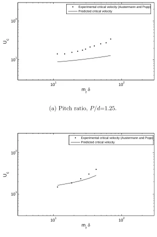
In order to validate the hybrid theoretical-CFD method, simulations of

the P/d= 1.25 and P/d= 1.375 arrays, matching the experimental setup of

number range of laboratory tests, (2.1×104 _{≤ Re ≤ 7.4×10}4_{). Using the}

values for dCL

dy and CD obtained from these simulations, the critical velocity

was calculated, for the appropriate mass ratio and a structural damping range

(mr = 493,0.02≤δ ≤0.14).

The comparison between the predictions and the experimental critical

velocities (Austermann and Popp, 1995) for the two P/d arrays is shown in

Fig. 6. Quantitatively, this methodology consistently under predicts the

crit-ical velocity for the P/d= 1.25 array, with a relative difference in the range

37% → 62%, while for the P/d = 1.375 array the relative differences are

somewhat lower, within a range of (0%→28%). There are two possibilities

for the deviation. Either the negative fluid damping is over predicted, which

is certainly possible given the embedded assumptions of the wake model.

Alternatively, the positive fluid damping associated with the drag may be

under-predicted. This is very likely as this effect is modeled with the

quasi-steady assumption as discussed above. In qualitative terms, the threshold

trend was captured for the two arrays. As the study envisioned here is

com-parative, focused on the trend rather than on the accuracy of the predictions,

it is concluded that the approach may be sufficient to conduct the parameter

dependency analysis proposed.

4. Sensitivity of the predicted critical velocity to parameter values

It is well known that the pitch ratio effects the critical velocity and has

been noted above, there is some evidence in the literature that the critical

impact of mass ratio is usually bundled into the mass-damping parameter,

but this implicitly assumes that damping and mass are equivalent. There

may be other non-dimensional numbers that may influence the critical

veloc-ity. One candidate might be the Stokes number. The Stokes number posed in

terms of the tube diameter is simply the ratio of Reynolds to critical velocity,

and as such is a ”twice reduced” quantity as Paidoussis et al. (2011) refer to

the mass-damping parameter, with the dependent quantity of interest (i.e.

the critical velocity) embedded in the parameter being varied. It should be

noted that although it is possible to construct a dimensionally correct

pa-rameter, it is not clear what length scale or time base should be used. Stokes

number finds application in the context of entrainment of particles (e.g. PIV

seeding) with the particle size as the length and so may be important in

two-phase flow in tube arrays, typical of flow in the center of steam generators.

However, this is beyond the scope of the current study, which will focus on

the Reynolds number.

Using the hybrid theoretical-CFD method described and validated above,

the effect of Reynolds number, mass ratio and pitch ratio (Re, mr, P/d) has

been estimated, and the relative importance assessed. Ninety steady

simula-tions, corresponding to the 5 pitch to diameter ratios (P/d= 1.25,1.30,1.32,1.375,1.44),

9 Reynolds numbers (Re= 104 →9×104) and two positions of the displaced

tube (±0.005d) were carried out. The resulting fluid force coefficients were

used in the quasi-unsteady model (Granger and Paidoussis, 1996; Meskell,

2009) with 7 mass ratios and 13 structural damping values. The combination

of these parameters produced 8190 stability thresholds estimates. Table 1

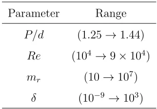
Parameter Range

P/d (1.25→1.44)

Re (104 _→9×104₎

mr (10→107)

δ (10−9 _→103₎

Table 1: Parameters range considered in the study of the critical velocity dependency.

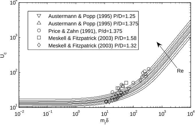
4.1. Effect of Reynolds number

The Reynolds number was varied in the steady CFD simulations by

al-most one order of magnitude from Re = 104 to Re = 9 ×104. This was

achieved by changing the onset flow velocity. Figure 7 shows the stability

threshold for the 9 Reynolds numbers considered, for a pitch ratio P/d =

1.375, and a mass ratio mr = 100. It was found that increased Reynolds

number increases the critical velocity over the entire stability threshold, and

this effect was seen for all pitch ratios. In the case shown in Fig. 7,

in-creasing the Reynolds number by a factor of 9 resulted in a factor of 1.6

increase in critical velocity at the lowest mass-damping value (mrδ= 10−2).

These results would indicate that the Reynolds number effect is moderate.

Furthermore, considering experimental or numerical inputs obtained at low

Reynolds numbers in the theoretical models, would yield conservative

esti-mates of critical velocity.

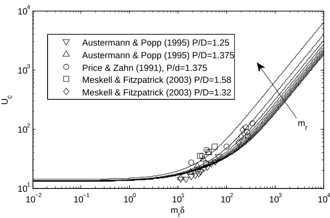
4.2. Effect of mass ratio

The simple time lag embedded in the quasi-steady theory Price and

mass and damping become combined into a single parameter, the so called

mass-damping parameter. This is actually the product of two independent

non-dimensional numbers: the mass ratio,mrand the logarithmic decrement,

δ. In the quasi-unsteady model Granger and Paidoussis (1996), the use of a

memory function means that the mass and the damping do not always

ap-pear together in the governing equation of motion. Thus, the mass-damping

parameter does not naturally appear in the coefficients of the characteristic

equation (Meskell, 2009). As a result, at a given value of mass-damping,mrδ,

the mass ratio mr may have a wide range of values. In order to assess the

effect of the varying the mass ratio, the critical velocity for the same array as

in Fig. 7 was assessed for 10≤mr ≤107 . The higher values of this range are

obviously unrealistic ( 104 would be a more realistic upper limit), but this

large range was use to achieve a comparable change in critical velocity to that

observed for the Reynolds number. Therefore, the first obvious conclusion

is that mass ratio is less significant than Reynolds number. However, it is

still worth considering if the mass ratio changes the effect of Reynolds

num-ber. In order to allow comparison of critical velocities for different Reynolds

numbers and mass ratios a renormalized critical velocity can be defined:

U_c∗ = Uc Ucref

= Uc

Uc(Re=5×104)

(8)

The reference value is chosen as the critical velocity at Re= 5×104 _{as this}

is the center of the Reynolds number range considered. Note that mass ratio

and structural damping are almost fixed for a given tube array installation,

but Reynolds number can be varied by the choice of flow velocity.

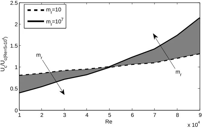
Fig-ure 9 shows the variation of the renormalized critical velocity over a range

associated with structural damping is δ = 0.1. As can be seen, the effect of

increasing Reynolds number is more-or-less linear, but increasing mass ratio

increases the sensitivity of critical velocity to Reynolds number: the slope of

the trend is steeper for high mass ratio.

Figure 10 shows the effect of varying the structural damping δ with a

fixed mass ratio mr = 100. The effect of varying Reynolds number is linear,

but again increased damping increases the sensitivity of critical velocity to

Reynolds number. However, the degree to which the slope of the trend is

changed by increasing damping is not as great. The fact that increasing

damping and increasing mass ratio act to move the critical velocity in the

same direction suggests that the two parameters can be combined in a single

parameter (i.e. the mass-damping parameter), but they are not completely

interchangeable, as increased damping has less effect than increased mass

ratio and this depends on the value of mass-damping parameter, as already

seen in Fig. 7.

In order to show the net effect of increasing the mr at a constant

mass-damping, the behaviour at three mass damping parameters (mrδ = 10−2,

mrδ = 104 and mrδ = 104) were calculated for increasingmr and decreasing

δ and is shown in Fig. 11. For the lowest mass-damping parameter value

(mrδ = 10−2) the variation of the critical velocity with Reynolds numbers

shows almost no dependency on mass ratio. As the mass-damping parameter

increases, the influence of mass ratio, mr, becomes stronger.

The range ofmr evaluated was extremely wide, spanning seven orders of

magnitude, and yet the effect on critical velocity is modest. Furthermore,

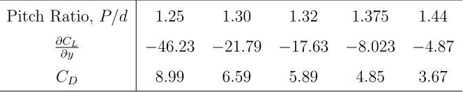
Pitch Ratio,P/d 1.25 1.30 1.32 1.375 1.44

∂CL

∂y −46.23 −21.79 −17.63 −8.023 −4.87

CD 8.99 6.59 5.89 4.85 3.67

Table 2: Fluid force coefficients for Re=5×104

the critical velocity, but this effect is confined to high values of mass-damping

parameter. At low values of mass-damping, where the critical velocity will be

lowest, the mass ratio has almost no effect. There is theoretical evidence (e.g.

Yetisir and Weaver, 1993b) that for high mass-damping values, damping

controlled FEI will occur at higher velocities than stiffness controlled FEI,

and so this would suggest that the effect of mass ratio might practically

be ignored. This explains why the widely adopted pragmatic approach to

consider the mass-damping parameter is actually valid, even though the mass

ratio and structural damping (logarithmic decrement) are separate physical

quantities.

4.3. Effect of pitch ratio

It is well known that pitch ratio is important for the critical velocity.

The mechanism for this dependency is that the static fluid force coefficients

depend strongly on the pitch ratio, for a given Reynolds number. For

exam-ple, Table 2 lists the fluid force coefficients obtained from the steady CFD

simulations for a Reynolds number of 5×104_.

The sensitivity of the critical velocity to pitch ratio has been evaluated

by considering five pitch ratios: P/d = 1.25,1.30,1.32,1.375 and 1.44. In

order to compare the behaviour of different pitch ratios at various Reynolds

this case, the reference value was critical velocity at P/d = 1.375, and the

particular Reynolds number.

U_c∗ = Uc Ucref

= Uc

Uc(P /d=1.375)

(9)

it was found that even after normalization with respect to the reference pitch

ratio (1.375), there was still a significant variation due to both Reynolds

num-ber and mass-damping parameter. Figure 12 shows the range of normalized

critical velocity U_c∗ for various pitch ratios over the range of Reynolds num-bers (104 _{≤ Re ≤ 9× 10}4_{). Note that the apparent lack of variation at}

P/d= 1.375 does not mean there is no variation with Reynolds number, but

rather that the dataset is referenced to this condition. The mass-damping

parameter considered is mrδ = 10. At the lowest Reynolds number (104)

the critical velocity for a pitch ratio of 1.25 is only 50% of what would be

expected in an array with a pitch ratio of 1.375. In comparison, Chen’s

em-pirical correlation Chen (1984) would yield a ratio of 74%. At the highest

Reynolds number (9× 104) for P/d = 1.44, the current study predicts a

ratio, U_c∗ of 120% , while Chen’s factor is 114%. The fact that the trend and order of magnitude are similar is encouraging, but there is significant

variation associated with Reynolds number. Furthermore, the variation with

Reynolds number depends on the mass-damping parameter. For this reason,

it has not been practical to develop a simple correction factor which

cap-tures the Reynolds number effect, the effect of pitch ratio and the effect of

5. Conclusions

A theoretical-CFD hybrid method has been proposed, in which force

co-efficients estimated in steady simulations are used as the inputs of the

quasi-unsteady model Granger and Paidoussis (1996) and combined with a

theo-retical memory function Meskell (2009). This allows predictions of critical

velocity without the need of any experimental data. Data from the literature

was used to validate the CFD simulations and the predictions obtained by the

hybrid theoretical-CFD approach. Results of these two comparisons showed

reasonable agreement in the pressure distribution in the tube surface and the

critical velocity predictions. However, as the discrepancy between the

exper-imental critical velocity and the predicted value is comparable in magnitude

to the variations observed, some caution must be exercised. Nonetheless,

using this approach the sensitivity of the predictions of critical velocity to

values of mass ratio, Reynolds number and pitch ratio was assessed. The

main conclusions derived from these studies were:

1. Reynolds number was found to increase levels of critical velocity for

the whole stability threshold, by as much as 60 % .

2. While mass ratio has an appreciable effect, it is relatively small, and so

it is reasonable to lump the mass ratio and structural damping together

in a single parameter, as is commonly done.

3. Pitch ratio was found to have the most significant effect, however, the

magnitude of the effect of pitch ratio depends on the Reynolds number.

Although work is need to improve the absolute accuracy of the predictions

quasi-usnteady formulation), the hybrid theoretical-CFD method has yielded some

useful insights into damping controlled FEI.

6. Acknowledgment

The authors gratefully acknowledge the financial support of: the

Princi-pality of Asturias Government under the PhD grant BP-12054 awarded to

Ms. de Pedro.

26th ITTC Specialist Committee on CFD, 2011. Practical guidelines for ship

cfd application. ITTC-Recommended Procedures and Guidelines.

Anderson, B., Hassan, M., Mohany, A., 2014. Modelling of fluidelastic

in-stability in a square inline tube array including the boundary layer effect.

Journal of Fluids and Structures. 132 (48), 362–375.

Austermann, R., Popp, K., 1995. Stability behaviour of a single flexible

cylin-der in rigid tube arrays of different geometry subjected to cross-flow.

Jour-nal of Fluids and Structures 9 (3), 303 – 322.

Chen, S., 1984. Guidelines for the instability flow velocity of tube arrays in

crossflow. Journal of Sound and Vibration 93, 439–455.

Chen, S. S., 1983. Instability mechanisms and stability criteria of a group

of circular cylinders subjected to cross-flow. part i: Theory. Journal of

Vibrations, Acoustics, Stress, Reliability and Design 105, 51–58.

de Pedro, B., Parrondo, J., Meskell, C., Oro, J., 2016. Cfd modelling of

forced vibrations or fluidelastic instability. Journal of Fluids and Structures

64, 67–86.

Gillen, S., Meskell, C., 2009. Numerical analysis of fluidelastic instability in

a normal triangular tube array. Proceedings of Flow Induced Vibrations.

Prague, Czech Republic.

Granger, S., Paidoussis, M., 1996. An improvement to the quasi-steady model

with application to cross-flow-induced vibration of tube arrays. Journal of

Fluid Mechanics 320, 163–184.

Harran, G., 2014. Influence of mass ratio on the fluidelastic instability of a

flexible cylinder in a bundle of rigid tubes. Journal of Fluids and Structures

47, 71–85.

Hassan, M., Gerber, A., Omar, H., 2010. Numerical estimation of

fluidelas-tic instability in tube arrays. Journal of Pressure and Vessel Technology

132 (4), 041307 (11 pp.) –.

Iacovides, H., Launder, B., West, A., 2014. A comparison and assessment

of approaches for modelling flow over. International Journal of Heat and

Fluid Flow 49, 69–79.

Keogh, D., Meskell, C., 2015. Bi-stable flow in parallel triangular tube arrays

with a pitch-to-diameter ratio of 1.375. Nuclear Engineering and Design

285, 98–108.

Khalifa, A., Weaver, D., Ziada, S., 2013. Modeling of the phase lag causing

fluidelastic instability in a parallel triangular tube array. Journal of Fluids

Lever, J., Weaver, D., 1986. On the stability of heat exchanger tube bundles.

part i: modified theoretical model. part ii: numerical results and

compar-ison with experiment. Journal of Sound and Vibration 107, 375–410.

Li, H., Mureithi, N., 2016. Development of a time delay formulation for

fluidelastic instability model. In: Flow-Induced Vibration and Noise 2016.

TNO, pp. 653–662.

Mahon, J., Meskell, C., 2009. Surface pressure distribution survey in normal

triangular tube arrays. Journal of Fluids and Structures 25, 1348–1368.

Mahon, J., Meskell, C., 2012. Surface pressure survey in a parallel triangular

tube array. Journal or Fluids and Structures 34, 123–137.

Mahon, J., Meskell, C., 2013. Estimation of the time delay associated with

damping controlled fluidelastic instability in a normal triangular tube

ar-ray. Journal of Pressure Vessel Technology, Transactions of the ASME

135 (3).

URL http://dx.doi.org/10.1115/1.4024144

Meskell, C., 2009. A new model for damping controlled fluidelastic instability

in heat exchanger tube arrays. Proceedings of the Institution of Mechanical

Engineers, Part A: Journal of Power and Energy 223 (4), 361–368.

Meskell, C., Fitzpatrick, J. A., 2003. Investigation of nonlinear behaviour

of damping controlled fluidelastic instability in a normal triangular tube

array. Journal of Fluids and Structures 18, 573–593.

vibrations of tube bundles in crossflow. In: Flow-induced vibration. I. Mech

E. London, pp. 231–242.

Paidoussis, M., Price, S., deLangre, E., 2011. FuidStructure Interactions

-Cross flow instabilities. Cambridge University Press, Cambridge.

Price, S. J., 1995. A review of theoretical models for fluidelastic instability of

cylinder arrays in cross-flow. Journal of Fluids and Structures 9, 463–518.

Price, S. J., 2001. An investigation on the use of connors’ equation to

pre-dict fluidelastic instability in cylinder arrays. Journal of Pressure Vessel

Technology 123, 448–453.

Price, S. J., Paidoussis, M. P., 1984. An improved mathematical model for

the stability of cylinder rows subject to cross-flow. Journal of Sound and

Vibration 97 (4), 615–640.

Saffman, P. G., 1992. Vortex Dynamics. Cambridge University Press.

Van Oudheusden, B., 1995. On the quasi-steady analysis of

one-degree-of-freedom galloping with combined translational and rotational effects.

Non-linear Dynamics 8 (4), 435–451.

Virgin, L. N., 2000. Introduction to experimental nonlinear dynamics : a

case study in mechanical vibration”. Cambridge Univeristy Press.

Yetisir, M., Weaver, D., 1993a. An unsteady theory for fluidelastic instability

in an array of flexible tubes in cross-flow. part i: Theory. Journal of Fluids

Yetisir, M., Weaver, D., 1993b. An unsteady theory for fluidelastic instability

in an array of flexible tubes in cross-flow. part ii: Results and comparison

with experiments. Journal of Fluids and Structures 7 (7), 767–783.

Zhang, Z., Zhao, C.-R., Yang, X.-T., Jiang, P.-X., Tu, J.-Y., Jiang, S.-Y.,

2017. Numerical study of the heat transfer and flow stability of water at

supercritical pressures in a vertical tube. Nuclear Engineering and Design

325, 1 – 11.

1st _{ORDER UNSTEADY}

WAKE MODEL (Meskell, C., 2009)

QUASI-STEADY THEORY (Granger, S. & Paidoussis,

M.P., 1996)

VALIDATION 2: EXPERIMENTAL CRITICAL VELOCITY

P/d=1.25, 1.375 Austermann, R. & Popp, K., 1994.

STRUCTURAL PARAMETERS

MEMORY FUNCTION FLUID DYNAMIC

COEFFICIENTS dCL/dy, CD CFD MODEL:

-STEADY -RANs

CRITICAL VELOCITY VALIDATION 1:

SURFACE PRESSURE Mahon, J. & Meskell, C.,

2009.

Re P/d

m_r d

Figure

2:

T

ypical

v

elo

cit

y

magnitude

con

tours

obtained

in

st

e

ady

sim

ulations

(

P

/d

=1.25,

U0

=0.89

P

d

9

d

9d

SD

Figure

3:

Sc

hematic

of

computational

Displaced

Tube

0 50 100 150 200 250 300 350 -1

-0.9 -0.8 -0.7 -0.6 -0.5 -0.4 -0.3 -0.2 -0.1 0

P*

 (º)

k- Standart k- RNG k- SST

Experimental data

Figure 5: Comparison of pressure coefficient,P∗, on tube surface computed from different

turbulence models, with experimental data Mahon and Meskell (2009). P/d = 1.32,

101 102 101

102

m

r

U c

Experimental critical velocity (Austermann and Popp) Predicted critical velocity

(a) Pitch ratio,P/d=1.25.

101 102 101

102

m

r

U c

Experimental critical velocity (Austermann and Popp) Predicted critical velocity

(b) Pitch ratio,P/d=1.375.

Figure 6: Comparison of critical velocity (Uc) predictions with experimental

10−2 10−1 100 101 102 103 104

101

102

103

104

m_rδ

U c

Austermann & Popp (1995) P/D=1.25 Austermann & Popp (1995) P/D=1.375 Price & Zahn (1991), P/d=1.375 Meskell & Fitzpatrick (2003) P/D=1.58 Meskell & Fitzpatrick (2003) P/D=1.32

Re

Figure 7: Effect of Reynolds number on the stability threshold, compared with

10−2 10−1 100 101 102 103 104

101

102

103

104

m_rδ

U c

Austermann & Popp (1995) P/D=1.25 Austermann & Popp (1995) P/D=1.375 Price & Zahn (1991), P/d=1.375 Meskell & Fitzpatrick (2003) P/D=1.58 Meskell & Fitzpatrick (2003) P/D=1.32

m_r

1 2 3 4 5 6 7 8 9

x 104

0 0.5 1 1.5 2 2.5

Re

U c

/U

c

(Re=5

×

10

4 )

m_r=10

m_r=107

m_r

m

r

1 2 3 4 5 6 7 8 9

x 104

0.4 0.6 0.8 1 1.2 1.4 1.6 1.8 2

Re

U c

/U

c

(Re=5

×

10

4 )

δ=10−4

δ=102

δ δ

1 2 3 4 5 6 7 8 9 x 104 0.4 0.6 0.8 1 1.2 1.4 1.6 1.8 2 2.2 2.4 Re U* c

m_r=107; m_r=104;

m

r=10 7_{; m}

r=10;

m

r=10 7_;m

r=10 -2_;

m

r=10; mr=10 4_;

m

r=10; mr=10;

m

r=10; mr=10 -2_;

m_r m_r

m_r=10

m_r=10-2

m_r=104

1.24 1.26 1.28 1.3 1.32 1.34 1.36 1.38 1.4 1.42 1.44 0.5

0.6 0.7 0.8 0.9 1 1.1 1.2 1.3

P/d

U c

*

Re=9104

Re=104

Re