High Accuracy Time of Flight Measurement Using Digital Signal Processing Techniques for Subsea Applications

doi:10.4236/jsip.2011.24047 Published Online November 2011 (http://www.SciRP.org/journal/jsip)

High Accuracy Time of Flight Measurement Using

Digital Signal Processing Techniques for Subsea

Applications

Muhammad Ashraf1, Hamza Qayyum1,2*

1

Department of Electronic Engineering, Mohammad Ali Jinnah University, Islamabad, Pakistan; 2Department of Physics, COMSATS Institute of Information Technology, Islamabad, Pakistan.

Email: *[email protected]

Received July 5th, 2011; revised September 5th, 2011; accepted September 17th, 2011.

ABSTRACT

The techniques widely used in ultrasonic measurements are based on the determination of the time of flight (T.o.F). A short train of waves is transmitted and same transducer is used for reception of the reflected signal for the pulse-echo measurement applications. The amplitude of the received waveform is an envelope which starts from zero reaches to a peak and then dies out. The echoes are mostly detected by simple threshold crossing technique, which is also cause of error. In this paper digital signal processing is used to calculate the time delay in reception i.e. T.o.F, for which a maximum similarity between the reference and the delayed echo signals is obtained. To observe the effect of phase un-certainties and frequency shifts (Doppler), this processing is carried out, both directly on the actual wave shape and after extracting the envelopes of the reference and delayed echo signals. Several digital signal processing algorithms are considered and the effects of different factors such as sampling rate, resolution of digitization and S/N ratio are analyzed. Result show accuracy, computing time and cost for different techniques.

Keywords: SONAR, Signal Processing, Time of Flight

1. Introduction

Ultrasonic sensors can be used to provide accurate dis-tance measurement at low cost, and are simple in constr- uction and mechanically robust. Often they can be used in environments where other sensors fail and are particul- arly well suited to subsea applications [1].

Major applications of the sensors may be found in the underwater Remotely Operated Vehicles (ROV) [2] for the purpose of obstacle avoidance and guidance control. Many methods are employed to generate ultrasonic wa- ves and currently continuous wave and pulse-echo techn- iques are widely used.

In continuous wave method, continuous signal is tran- smitted whose echo is received by a separate receiver us- ing separate transducers for transmission and reception. A complex hardware is required in order to determine number of integer wavelengths in the phase shift.

Pulse-echo techniques [3] are mostly used in Sonar’s and other industrial applications. A short train of waves is generated, enabling the same transducer to be used both for transmission and reception. This wave as echo is

reflected by the target and a portion of which is captured by the transducer. The time of flight of the transmitted signal waveform is determined and the distance between the transducer and target is given as follows.

0 2

D cT (1)

where D = distance from transducer to target, T0 = time of flight and c = velocity of ultrasound [3].

Accuracy of the measurement depends on the knowl-edge of c and the correct estimation of T0. The sound velocity shows an almost linear dependence with tem-perature (2) which can be easily compensated [4].

2

1410 4.21 0.037 0.0175 1.14

c  T T  d sm/sec(2)

where “T” is the water temperature in ˚C, “d” is the depth in metres and ‘s’ is the salinity in grams of salt per litre of water.



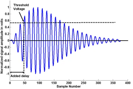
idth ultrasonic transducers used for subsea applications. In fact, the received echoes cross the threshold level after some time delay (i.e. after the exact beginning due to processing delays), as shown in Figure1, making the target to appear slightly farther away than it actually is. This error could be avoided if the added delays were constant, but the amplitude changes produce deviations. To quantify this error, the echo waves can be modeled as the damped sinusoids [3,4].

 

 



v t a t t (3)

where [5], the values for “m” range between 1and 3 and provide good approximations, “h” and the phase shift “” are transducer dependent cons- tants and “ωc”is the angular frequency of the ultrasound.

 

0

m t h a t _v t e

On the other hand, echo amplitude change with dist- ance “D”due to beam spreading and attenuation is given by [6]:

 

0

D

v D V e D (4) where “” is the coefficient of attenuation which is

15 2

69.5 10  f dB/m) [7] in water.

Constant added delays can be obtained by doing varia- ble matching Equation (4) with D of the echo produced by the targets at different distances. However, there are other causes of echo amplitude variations which cannot be easily modeled, such as the size, shape and attitude of the targets.

The noisy acoustical voltage waveform v(t), received as delayed echo signal can always be modeled in the time domain as the superposition of two events:

V(t) = s(t) + n(t)

where s(t)is the delayed echo signal and n(t)is the am-bient ocean noise.

The signal enhancement (improvement in the sig-nal-to-noise ratio) [8,9] can be achieved by DSP algor- ithms used to average out the noise component of the

Figure 1. Reference echo signal of the 6 KHz underwater acoustic transducer.

waveform so that only the signal is left. Assuming that the noise level is a fraction of maximum amplitude of the echo, it is found that an uncertainty of 2Tr is produced in

the echo arrival time [6]. With S/N ratio of –20 dB this adds a few meters to the error. In short, the cumulative error of the threshold technique is [6]:





    (5) where “ ” is fractional index and can be calculated from the samples of correlation values [3].

2. Measurement Algorithms

The model of the echo waveform is given as in Equation (3). It would be easy to compute the starting time of the echo pulse by locating the maximum of the envelope. The relative variation of the waveform amplitude is rather low at the maximum of the envelope, so that a small noise spike could produce a false maximum. On the other hand, the largest relative amplitude variation is found at the origin of the echo pulse, where the value of echo signal is very low that makes the S/N ratio poorer. Nevertheless this suggests that if many sampling points of the signals were considered, it would be possible to adjust the received echo to the model, obtaining the starting time accurately.

The signal corresponding to the delayed echo is the result of the double conversion process. In fact, the elec-trical signal applied to the transmitter is converted into an acoustic wave and the acoustic echo is converted back into an electrical signal. There is a difference between the wave shapes of the transmitted and the delayed echo signals, due to the electric impedance of the transmitter and receiver circuits and the transducer bandwidth. The transmitted signal is not used in the digital signal proc-essing algorithms for obtaining the starting time accuracy due to the difference in the shapes of the transmitted and the delayed echo signal.

An exact mathematical modeling of the delayed echo waveform for a given transducer is not essential. All ra- nge measurements can be made relative to the position of a reference target, whose absolute distance to the trans- ducer is accurately known. Therefore, the theoretical waveform model given as in Equation (3) can be re-placed by the reference echo signal waveform received from the reference target.

In this paper the echo received from a reference target is used as a reference signal. The methods considered include norms L1 and L2, and correlation. They search the delay values for which a maximum similarity betw- een the reference and the echo signals are obtained. To observe the effect of phase uncertainties and frequency shifts, this processing is carried out both on the actual wave shape and the extracted envelope of the signals.

iers followed by low pass filters introduces some delay. Different digital signal processing algorithms have al-ready been reported, which eliminate the delay [6].

The Hilbert Transform technique has been used in this paper and the steps needed are as follows:

1) Obtained the Fourier transform of the sampled echo using a complex FFTutility,

2) Set all negative frequency components to zero and double the positive frequency components

3) Magnitude of the inverse FFT yields the envelope. The function “x(k)” of the basic digital signal process-ing algorithms are:

 



  

1

L1 norm:

N

i

x k e k i r







 



  

1 L2 norm:

N

i

x k e k i r i







 



  

1

Correlation:

N

i

x k e k i r







The delay value (T0) where the greatest similarity be-tween the reference and delayed echo signal is found corresponds to the index “K0” which makes “x(k)” mini-mum in Equations (6)-(7) and maximini-mum in (8).

3. Simulation Results for the Basic

Algorithms

The simulation is done using 6-KHz underwater acoustic transducer that acts both as a transmitter and receiver, converting an electrical signal into an acoustical one and vice versa. Signals received from the transducer are fil-tered by a bandpass amplifier whose centre frequency is synchronous with the transducer operating frequency. The results of the simulations are shown and discussed below.

3.1. Results of Correlation, L1 Norm and L2 Norm

The Figure 2(a) shows the reference signal, the delayed echo signal and the processed correlation, L1 Norm and L2 Norm directly without envelope extraction. The de-layed echo signal is dede-layed by 88 samples, sampling rate is 60,000 samples/sec with a phase difference of 2400 (1.1111e–005 sec) which present a T.o.F equal to 0.001477 sec and corresponding distance from the target is equal to 1.1083 meters. It can be seen that the proc-essed output which is maximum of the correlation and minimum of both L1 and L2 Norms show a delay of 87samples. There is an error of one sampling interval added to phase shift. That is due to the phase difference of the delayed echo signal with respect to the reference signal. Actual distance from the target is 1.1083 meters and that calculated by using DSP algorithms is 1.0875 meters. There is an error of 20.83 mm by processing the

actual echo signals.

The extracted envelopes of the reference and the de-layed echo signals are shown in Figure 2(b). The lower three plots are the outputs of the correlation, L1 Norm and L2 Norm algorithms performed on the extracted en-velopes. It can be seen that the processed output which is maximum of the correlation and minimum of both L1 and L2 Norms show a delay of 88 samples.

There is an error of only a phase shift. That is due to the phase difference of the delayed echo signal with respect to the reference signal. Actual distance from the target is 1.1083 meters and that calculated by using DSP algori- thms is 1.100 meters which gives an error of 8.33 mm.

3.2. Sampling Frequency

The normalized sampling frequency is the ratio of the sampling rate with respect to the signal frequency. It presents number of samples taken for each cycle. The effect of this parameter without envelope extraction is shown in Figure3(a). For L1 and L2 algorithms the er-ror reduces monotonically but non-linearly. In case of correlation the error reduces linearly and for the meas-urement using delay of the maximum values of reference and delayed echo (MVRE) signals the error is non-linear and do not reduce monotonically.

In Figure3(b) the simulation is shown with the same reference and delayed echoes but the processing includes envelope extraction also. It can be seen that for L1 and L2 algorithms, the error remains rather constant if the ratio Fs/F becomes higher. In case of correlation the error is very high when the ratio Fs/F is less than 3 and it then reduces for the higher values. For MVRE signal there is very small variation in the error.

3.3. Noise

The performance of different DSP algorithms is shown in Figure 4(a) without envelope extraction. L1 and L2 norms show large error at low signal to noise ratio (S/N). The error due to correlation is almost constant. The MVRE algorithms show very small error and the change in error is also very small.

The performance of different DSP algorithms is shown in Figure4(b) with envelope extraction. L1 norms show increase in error at higher signal to noise ratio (S/N). There is a small variation in the error due to correlation and L2 norm. The MVRE algorithms show very small error till S/N ratio is less than 0.5 and the error becomes more than 2.5 meters for less values of S/N ratio.

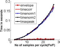
3.4. Computing Time

(a)

(b)

Figure 2. Waveforms of the received and processed signals. (a) without envelope extraction, (b) after envelope extraction.

(a)

(b)

Figure 3. Plot of measurement error against Fs/F (a) with-out envelope extraction, (b) with envelope extraction.

(a)

(b)

Figure 4. Plot of measured error against S/N ratio (a) with out envelope extraction, (b) with envelope extraction.

Figure 5. The computing time for the different processing algorithms.

more time as compared to other algorithms. The standard Matlab algorithm which is the fast correlation algorithm, requires less time, therefore standard function is not used for the calculation of correlation. Peak detection algorithm requires the least time as compared to other processing algorithms.

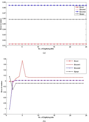
3.5. Resolution of the Digitizing Process

The effect of ADC resolution is shown in Figure 6(a) below. The error due to all the algorithms remains same. There is no effect of variation in ADC resolution if the processing is done without envelope extraction.

(a)

(b)

Figure 6. Resolution of the Digitizing Process (a) without envelope extraction and (b) with envelope extraction.

than 2 bits resolution. Error due to L2 norm becomes constant for resolution of more than 8 bits.

4. Conclusions

Several DSP methods have been analyzed and compared with respect to error in rage measurement and computa-tion time. The range error in simple threshold deteccomputa-tion method goes up to half metres. The threshold level sho- uld be at least 5 times more than the peak value of the noise signal present in the echo signal. The range can not be detected if the S/N ratio is less than 5. Using DSP methods range can be measured for a S/N ratio of 0.1 with an error less than a metre.

Correlation is the best method with low S/N ratio and low digitizing bits.

L2 norm provide better results with low noise level, although it requires high sampling frequency, high

digi-tizing resolution and higher computing time to achieve its full performance.

L1 norm provide almost same results as L2 norm but it requires simplest hardware for the computation of the algorithm.

The MVRE algorithms also show better results but gives higher error at lower till S/N ratio.

It is seen that the processing after envelope extraction gives the best results in term of sampling frequency, Resolution of the Digitizing and S/N ratio.

Digital processing using cross correlation algorithm with 1bit digitizing resolution and processing after enve-lope extraction gives the best results.

REFERENCES

[2] J. L. Sutton, “Under Water Acoustic Imaging,”

Proceed-ings of the IEEE, Vol. 67, No. 4, 1979, pp. 554-566.

doi:10.1109/PROC.1979.11283

[3] D. Marioli, C. Narduzzi, C. Offelli, D. Petri, E. Sardini, and A. Taroni, “Digital Time of Flight Measurement for Ultrasonic Sensors,” IEEE Transactions on

Instrumenta-tion and Measurement, Vol. 41. No. 1, 1992, pp. 93-97.

doi:10.1109/19.126639

[4] V. A. Krasilnikov, “Sound and Ultrasound Waves,” 3rd Edition, Washington, 1963, p. 167.

[5] C. E. Tibbs and G. G. Johnstone, “Frequency Modulation Engineering,” Chapman and Hall Ltd., London, Chap. 2, 1956.

[6] M. Parrilla, J. J. Anaya and C. Fritsch, “Digital Signal Processing Techniques for High Accuracy Ultrasonic Range Measurements,” IEEE Transactions on Instrumentation

and Measurement, Vol. 40. No. 4, 1991, pp. 759-769.

doi:10.1109/19.85348

[7] J. Blitz, “Fundamentals of Ultrasonics,” Butterworths, London, Chap. 5, 1967.

[8] F. G. Stremler, “Introduction to Communication Systems,” 3rd Edition, Addison-Wesley Publishing Co., 1990, pp. 195-197.