ISSN Online: 2160-0406 ISSN Print: 2160-0392
Modeling and Simulation of Two-Staged
Separation Process for an Onshore Early
Production Facility
Ojo Ademola, J. G. Akpa, K. K. Dagde
Department of Chemical Engineering, Rivers State University, Port Harcourt, Nigeria
Abstract
Early Production Facilities are makeshift process deployment that ensures that marginal oilfield operators make revenues from their new discoveries with little cash outlay and limited investment risks. Authors have in past si-mulated a gas process facility using Hysys without particularly developing mathematical models for the key equipment. There also has been modeling of phase separation dynamics and process simulation but still without models for equipment. We basically developed models for the critical process equip-ment for early production, sized the equipequip-ment with data from a marginal field in the Niger delta region of Nigeria and then ran a dynamic simulation with the sized equipment. The important elements of the deployment are two-phase process vessel, 3-phase process vessel; knock-out drum, produced water treatment unit. Mathematical models were developed and adapted with Mathlab for the equipment sizing whilst ASPEN PLUS was used for simulating the process. Process data retrieved from a marginal field in Nigeria was used as input to quantify the equipment models. Sized equipment was deployed in Hysys V8.8 for a steady and dynamic state. The system simulation was com-prised of a two-phase process vessel followed by a 3-phase process vessel [1]. The unwanted gas was sent to knock out drum for removal of entrained liq-uid droplets before flaring (this was because the volume of gas processed is deemed uneconomical) and produced water to treatment unit for removing droplets of oil before disposal. Gas, oil and water were fed into the first stage separator (2-phase) at 132918.34 Ibmole/hr, 7622.95 Ibmole/hr and 1082.74 Ibmole/hr respectively. The operating pressures of the first and second vessels were at 850 psi and 150 psi respectively. The 2-phase vessel flashed off 96.7% of the gas and increased the liquid recovery by 3.3%. At the end of the second stage separation, oil yield increased by 270 Ibmole/hr, the gas increased by 110.15 Ibmole/hr whilst water reduced by 379 Ibmole/hr. This result
con-How to cite this paper: Ademola, O., Akpa, J.G. and Dagde, K.K. (2019) Model-ing and Simulation of Two-Staged Separation Process for an Onshore Early Production Facility. Advances in Chemical Engineering and Science, 9, 127-142.
https://doi.org/10.4236/aces.2019.92010
Received: January 7, 2019 Accepted: January 29, 2019 Published: February 1, 2019
Copyright © 2019 by author(s) and Scientific Research Publishing Inc. This work is licensed under the Creative Commons Attribution International License (CC BY 4.0).
http://creativecommons.org/licenses/by/4.0/
Open Access
firmed that the vessels were sized to optimize recovery of hydrocarbons en-trained in the various phases into the most required oil phase.
Keywords
Modeling and Simulation, 2-Phase Process Vessel, 3-Phase Process Vessel, Effective Length, Seam-Seam Length, Slenderness Ratio
1. Introduction
Oil exploration is a capital intensive investment. It comes with a lot of cash out-lay requirements before generation of economic returns or bottomline. In the Nigerian context, Marginal fields are deemed economically viable and licenses are always allocated to locals. Sometimes they are referred to as marginal when they constitute a divested asset from a major international oil company such as Shell, Chevron, Agip, Total etc. whilst other times they are unexplored oil blocks with average reservoir capacity from seismic studies [2]. The challenge of devel-oping a marginal field often lies in accessibility of funds ranging from those re-quired for drilling, completions, and constructing of surface production facilities to operational services. Experience has shown that the delays between approvals of licenses to realization of full field optimization are a direct consequence of lack of funds. The cost of field development is quite high. Many marginal fields after drilling and completions are left for as long as ten years trying to source for funds to construct the crude process facility. The essence of this study is to de-sign and test by simulating a makeshift crude process facility that will greatly reduce the cash outlay requirement and bring first oil realization to fruition quickly. With the solution proffered, marginal field operators can quickly con-vert their existing reservoir asset to cash whilst planning expansion or full field development. It will simply ensure the operators have cash generation from their assets in order to fund the field development. This ideally is every investor’s dream.
Crude oil production operation is key to the petroleum and gas industry as its efficiency determines the quality of the crude and ultimately the economics of it all. Surface production operation is basically a set of unit operations required to treat crude oil to meet certain export requirements and also ensure that the set of activities required to achieve these is environmental friendly and poses to health and safety threat to human and animal life.
The concept of this study is to flow multiphase well fluid from the well through four basic process vessels with different handling capacities. The vessels were sized based on envisaged fluid flow characteristics and rates. The bulk liq-uid hydrocarbon was the content of interest and was passed through a three-stage separation process. The first stage was comprised of a two-phase se-parator i.e. separates fluid into gas and liquid phases. Phase equilibrium dynam-ics guides the bulk of the separation by flashing of the vapor out of the liquid
phase. Separation degree of the vapor phase was expected to be at 96% - 98% depending on nature of the multiphase whilst the remaining vapor % was re-tained in the liquid phase [3]. This stage vessel was operated at a much higher pressure and it will present unstable crude to the next process stage.
The second process stage was comprised of a three-phase separator that sepa-rated the fluid into three phases i.e. oil, gas and water. The separator was oper-ated at a much lower pressure and at reduced fluid velocity ensuring that the unstable light hydrocarbons in the liquid phase becomes stable and flashes into the gas phase [4]. About 3% entrained gas in the liquid phase was dislodged into the vapor phase. This ensures that the vapor pressure of the liquid was consi-derably reduced in order to reduce volatility and explosive tendencies of the crude oil [5]. Causing a change in thermodynamic property of the fluid mixture here supports the kind of separation expected. Retention time of the fluid in the vessel played a vital role in aiding the separation of the oil from the water. Prac-tically, this was achieved by allowing a reasonably high vapor liquid interface height in the vessel and operating the vessel at a relatively low pressure. All these conditions ensured that the fluid phases were adequately in contact with each other resulting to phase equilibriums and other conditions necessary to cause separation by gravity [4].
Some of the export requirements for crude oil are the basic sediment and wa-ter (BS & W) content which must be less than 0.5%, the vapor pressure which must be considerably about the Reid’s vapor pressure (Absolute pressure of the vapor of the crude oil at 37.8˚C following the ASTM-D323 test method). RVP is also a function of measure of the stability of the crude oil [4]. It ensures that the volatility is reasonably within a limit that the crude can be safely pumped and transported through pipelines at prevailing environmental conditions without constituting explosive mixtures. Environmental impact control of the crude process operation includes the treatment of the produced water to remove the oil droplets entrained with it. The presence of oil in water at disposal would cause harm to aquatic and plant lives. It reduces the amount of oxygen present in the water bodies for aquatic lives to live thereby impacting on their lives. Presence of crude oil in water disposed of on land interfered with the efficacy of the soil nutrient thereby reducing or completely eliminating soil yield. The droplets of liquid entrained in the continuous gas phase to the flare was removed to ensure gas burns completely and efficiently without deposition of carbon on land that may cause harmful impact of soil fertility and crop survival [6].
Some work has been done in this regards in the past.
2. Models Development
The following assumptions were made in the design and simulation of the process: • The multiphase mixture is without foam and emulsion, conditions that would
drastically cause an extension of the retention times required.
• The pour and hydrate points of the liquid hydrocarbon are reasonably below
the operating temperatures of all vessels. These ensure no wax or hydrate formation and eliminate the need for chemical injection.
• The smallest separable liquid droplet from all phases is in order of 500 µm. • The liquid carry over in the gas line is negligible and insignificant.
2.1. Gravity Settling Model
Phase separation is largely done under influence of gravity as supported by Stoke’s law. However, the law has different regimes and does not guide all sepa-ration cases.
The separation envisaged here is of liquid droplets settling through the pre-vailing continuous phase of either gas or oil. Inside the two phase vessel, it is en-visaged that the liquid droplets (oil and water) will settle through the continuous gas phase to ensure two phase separation. In fluid mechanics, that liquid droplet will settle with a terminal velocity under influences of the drag and buoyant forces.
2
2t
D D g V
F C A
g
ρ
=
(1)
where FD is the Drag Force, Ib, CD is the drag coefficient, A is the area of the
liq-uid droplet, ft2
g
ρ
is the density of the gas medium, Ib/ft3, Vt is the terminal
velocity in ft/s, g is the gravitational acceleration at 32.2 ft/s2.
When the flow is laminar, then the Stoke’s law is effective and the quantity CD
is given thus:
24 D
C Re
= (2)
g t
g
DV
Re=ρµ (3)
Substituting Equation (2) and Equation (3) into Equation (1) and simplifying yields:
2 2
24 π
4 2t
D g
g
g
V D
F DV
g
ρ ρ
µ
=
(4)
Essentially, the droplet continue to accelerate until a terminal velocity is reached at which point the drag force equates the buoyancy force from the prin-ciple of Achimedes. It is also assumed that the Stoke’s law can guide the droplet movement when the flow is laminar in nature and therefore
3π
D t
F = µ′DV (5)
Again the Bouyancy force acting on the body from the principle of Achimedes is given thus:
(
)
π63B l g D
F =
ρ ρ
− (6)Equating Equation (5) and Equation (6) and simplifying for Vt, we have the
following equation:
2 18
l g
t
V ρ ρ D
µ −
=
(7)
where: D = Liquid droplet diameter, ft, µ' = µ (2.088 × 10⁻⁵), Viscosity in cp, D = dm (3.281 × 10⁻⁶), ρ =l 62.4×S G. , ρ =g 62.4×S G. .
Therefore Equation (7) simplifies as:
(
)
6 2
1.78 10 .
t
S G dm V
µ
−
× ∆
= (8)
Practically in the industrial situations, the flows are not always laminar and it becomes difficult for the Stoke’s law to guide. Hence the following expression for
CD suffices:
1 2
24 3 0.34
D
C Re
Re
= + + (9)
Substituting Equation (9) into Equation (2) and then equating FB and FD then
simplifying will yield the desired applicable Vt in practical scenarios. 1
2
l g m
t g D d V C ρ ρ ρ − =
(10)
2.2. Model Development for a 2-Phase Process Vessel
2.2.1. Gas Capacity Constraint
Basically two constraints govern process vessel design:
• Gas Capacity constraint which ensures that the liquid droplet is permitted to settle by gravity according to Equation (10) through the continuous gas phase. • Liquid Capacity Constraint which must be sufficient enough to allow
liq-uid-liquid equilibrium for separation to occur.
The designs are for assumed situations when the vessels are operated half filled with liquid.
Assuming Ag is the area of the vessel occupied by gas in ft2, Vg is the velocity
of the gas in ft/s and Q is the flow rate in ft3/s:
g g
Q V
A
= (11)
2 2
2
1 π 1 π
2 4 2 4 144 367
g d d
A = D = =
(12)
Qg is in MMSCfd
6 SCF day hr 14.7
10
MMSCF 24 hr 3600 s 520
0.327 g g TZ Q Q P TZ Q P = × × × × × = (13)
Substituting Equation (12) and Equation (13) into Equation (11) yields
(
)
20.327 g 367
g TZ Q P V d = 2 120 g g TZQ V Pd
= (14)
If we set the residence time of the gas to be the time required for a liquid droplet in its continuous phase to settle down to the gas liquid interface, then:
eff g g L t V
= (15)
Residence time of gas
2 d t D t V
= converting D in ft to d in inches
24 d t d t V ∴ = :
Time required for a liquid droplet to settle down to the gas-oil interface tg =
res-idence time of gas; td= time necessary for a liquid droplet to settle from
consti-nuos gas phase to gas liquid interface.
2 120 eff g g L t TZQ Pd = : 1 2
0.0119 l g
t g D dm V C ρ ρ ρ − =
If tg= td with simplification
1 2
420 g g D
eff
l g m
TZQ C dl P d ρ ρ ρ = −
(16)
2.2.2. Liquid Capacity Constraint
For a liquid droplet settling through a continuous fluid phase with a retention time t in second, the following expression finds relevance:
V t
Q
= (17)
where 1π 2 2.73 103 2
2 4D eff eff
Vol= l = × − d L
3
1 5
1 5.61barrel 24 hr 3600 sft day hr 6.49 10 1
Q Q= × × × ≠ × − Q
2
1 42.0d Leff
t
Q
= (18)
2
0.7r l
eff t Q
d L = (19)
tr = Desired retention time for the liquid, min; Ql= Liquid flow rate in bpd. 2.2.3. Seam to Seam Length
D and Leff are the vessel diameter and effective length respectively. However, in
order to ensure incorporation of useful and important control mechanisms, the vessel length has to be slightly extended to accommodate for the instruments [3] [4].
12
ss eff d
L =L + (20)
And
4 3
ss eff
L = L (21)
Equation (18) suffices for cases of Gas Capacity governing the design whilst Equation (19) suffices in event of Liquid Capacity governed designs.
2.3. Three Phase Process Vessel Design
The bulk liquid separation and flashing of the retained 3% gas in the stream takes place in the gravity section of the 3-phase process vessel. A gas and liquid capacity constraint also governs the design of the vessel here.
2.3.1. Gas Capacity Constraint
Liquid droplets separates out under the medium influence of forces in the con-tinuous gas phase and the phenomenon is same for both the two and three phase process vessels. Hence Equation (16) remains valid
1 2
420 g g D
eff
l g m
TZQ C
dL
P d
ρ ρ ρ
=
−
(22)
2.3.2. Liquid Capacity Constraint
Also referred to as retention time constraint starts off with an expression of re-tention time for the liquids to separate out of the bulk three phase fluid interac-tion.
Vol t
Q
=
And 1 π 2
( )( )( )
π 2 2.73 103 22 D4 eff 2 4 144d eff
Vol= L = × − d L
( )
2.73 103 2 oeff o
l
A
Vol d L
A
−
= ×
(23)
( )
2.73 10 3 2 weff w
l
A
Vol d L
A
−
= ×
(24)
And QD and Qw are both in bpd
3
5
ft day hr
5.61 6.49 10
banel 24 hr 3600 s
o o
Q Q= × × × = × − Q
5 6.49 10 w
Q= × − Q
Ao, Aw and Al are cross sectional areas of oil, water and liquid respectively.
2 2
1
42 o o o ; 42 w w w
I eff eff
A t Q A t Q
A d L A d L
= =
(tr)o and (tr)w are in minutes
( )
( )
2 2
1
0.7 o r o o; 0.7 w r w w
I eff eff
t Q t Q
A A
A d L A d L
= =
( )
( )
2 1.42eff r o o r w w
d L = t Q + t Q (25)
where Qw = water flow rate, bpd, (tr)w = water retention time, minutes, Qo= Oil
flow rate, bpd, (tr)o = Oil retention time, minutes
To ensure that 500-micron of water droplet are permitted to settle out of oil pad, the oil pad thickness has to be constrained thus;
12 o w t h t V
= (26)
where t 1.78 106
(
.)
2S G dm V
µ
−
× ∆
=
(
)
246800 :
.
o
w w o
h
t t t
S G dm
µ
= =
∆
( )
60o r o
t = t
(
)
2( )
46800 60
. ho tr o
S G dm
µ
∆( ) (
)
20.00128 r o . o
t S G dm
h = µ ∆ (27)
Above equation must be satisfied for water droplet to settle out of oil. ho is the max thickness for this to be valid.
For dm = 500 micron
( )
320( ) (
r o .)
o masst S G
h
µ
∆= (28)
tr is in minutes, tw, to are in seconds, V is in ft/s, ho is in inches, dm is in micron, µ
is in cp.
Similarly, for given oil retention time and water retention time, (ho)max
con-straint establishes max concon-straint establishes maximum diameter thus:
t eff Q A L = 5 6.49 10 o
Q= × − Q 5 6.49 10 w
Q= × − Q
( )
60o r o
t = t
( )
60 r wt= t
( )
3 3.89 10 o r o o eff Q t A L − = ×( )
33.89 10 w r w w eff Q t A L − = ×
(
)
2 o w
A= A A+
( )
( )
( )
0.5 w r
w w
r o o r w w
Q t A
A t Q t Q
=
+
(29)
The fraction of vessel cross-sectional area occupied by water
( )
max max oh d
β
=1 o
h d
β = (30)
2.3.3. Seam-Seam Length and Slenderness Ratio
The essence and method of determination of seam to seam lengths and slender-ness ratio is same for process vessels. Slenderslender-ness ratio is practically limited to 3 - 4 for prevention of re-entrainment of liquid at the gas/liquid interface.
Slenderness ratio higher than 4 can be slightly acceptable for three-phase process vessel, when the gas content is small.
3. Results and Discussions
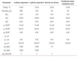
The models developed for each of the vessels were solved using Mathlab whilst the simulation was performed with Aspen Hysys v8.8. Process vessels are speci-fied by their diameter in inches and length in feet. Standardly, the vessels di-ameter is expanded in 6 “increments whilst the lengths are expanded in 2.5” in-crements [7] [8]. Data (compositional Feed characteristics and equipment pa-rameters) were taken from a marginal field in the Niger Delta Oil producing area of Nigeria to size the equipment and run the simulation. These are shown in Ta-ble 1 and Table 2.
The feed input to Hysys requires compositional analysis of all streams. These data were deployed for the simulation of the process.
This second set of bulk fluid data were used as equipment sizing parameters for the two vessels.
3.1. Two Phase Process Vessel Sizing
Table 3 shows standard vessel sizes available in the industry and from where reference would be drawn in our sizing
1) The Drag Coefficient CD was calculated at few iterative steps using Mathlab CD = 0.829
2) Gas Capacity Constraint
dLeff= 3.5478
The Gas Capacity Constraint apparently will not govern due its relatively low value.
3) Liquid Capacity Constraint
d2L
eff = 21429.
This quantity will govern due to its realistic value.
Table 1. Compositional feed characteristics.
SN Components Gas Stream % Oil Stream % Water Stream %
1 N2 0.04 0.00 0.05
2 CO2 1.13 0.00 0.10
3 H2O 0.01 0.00 97.03
4 C1 85.21 5.00 0.05
5 C2 6.34 0.01 0.17
6 C3 4.1 0.01 1.3
7 i-C4 0.87 0.01 1.3
8 n-C4 1.36 0.02 0.00
9 i-C5 0.43 0.02 0.00
10 n-C5 0.36 0.03 0.00
11 C6 0.11 0.10 0.00
12 C7 0.03 90.12 0.00
13 C8 0.01 0.08 0.00
14 C9 0.00 0.60 0.00
15 C10 0.00 2.0 0.00
16 C11 0.00 2.0 0.00
Flow Parameters
Pressure (psi) 900 900 900
Temperature (˚F) 118.4 118.4 118.4
Viscosity (cp) 0.0119 1.01
Specific Gravity 0.65 0.825 1.07
Flow rates 3 7500 1500
Table 2. Equipment input design parameters.
Parameter 2-phase separator 3-phase separator Knock out drum Produced water treatment unit
Temp, ˚F 118.4 118.4 118.4 118.4
Pressure, psi 900 150 50 50
SGw 1.07 1.07 1.07 1.07
SGo 0.825 0.825 0.825 0.825
SGg 0.65 0.65 0.65 0.65
ρo, Ib/ft3 51.48 51.48 51.48 51.48
ρw, Ib/ft3 66.76 66.76 66.76 66.76
ρg, Ib/ft3 4.02 4.02 4.02 4.02
µo, cp
µw, cp 1.01 1.01 1.01 1.01
µg, cp 0.0119 0.0119 0.0119 0.0119
Qo, bpd 7500 7500 7.5
Qw, bpd 1500 1500
Qg, mmscfd 3 3 3
[image:10.595.210.540.483.735.2]Table 3. Standard horizontal process vessel sizes [4] [9].
Size [D(inch) by L(ft)] Maximum Allowable Working Pressures (PSI) @100˚F
16” × 5’ 230 600 1000 1440 2000
16” × 71/2’ 230 600 1000 1440 2000
16” × 10’ 230 600 1000 1440 2000
20” × 5’ 230 600 1000 1440 2000
20” × 71/2’ 230 600 1000 1440 2000
20” × 10’ 230 600 1000 1440 2000
24” × 5’ 125 230 600 1000 1440 2000
24” × 71/2’ 125 230 600 1000 1440 2000
24” × 10” 125 230 600 1000 1440 2000
30” × 5’ 125 230 600 1000 1440 2000
30” × 71/2’ 125 230 600 1000 1440 2000
30” × 10’ 125 230 600 1000 1440 2000
36” × 5’ 125 230 600 1000 1440 2000
36” × 71/2’ 125 230 600 1000 1440 2000
36” × 10’ 125 230 600 1000 1440 2000
36” × 15’ 125 230 600 1000 1440 2000
42” × 71/2’ 125 230 600 1000 1440 2000
42” × 10’ 125 230 600 1000 1440 2000
42” × 15’ 125 230 600 1000 1440 2000
48” × 71/2’ 125 230 600 1000 1440 2000
48” × 10’ 125 230 600 1000 1440 2000
48” × 15’ 125 230 600 1000 1440 2000
54” × 71/2’ 125 230 600 1000 1440 2000
54” × 10’ 125 230 600 1000 1440 2000
54” × 15’ 125 230 600 1000 1440 2000
54” × 20’ 125 230 600 1000 1440 2000
60” × 10’ 125 230 600 1000 1440 2000
60” × 15’ 125 230 600 1000 1440 2000
60” × 20’ 125 230 600 1000 1440 2000
66” × 15’ 125 230 600 1000 1440 2000
66” × 20’ 125 230 600 1000 1440 2000
66” × 221/2’ 125 230 600 1000 1440 2000
72” × 15’ 125 230 600 1000 1440 2000
72” × 20’ 125 230 600 1000 1440 2000
72” × 221/2’ 125 230 600 1000 1440 2000
4) Estimation of the Seam to Seam Length based on the governing liquid capacity constraint must provide a value between 3 and 4 to eliminate re-entrainment
dencies.
Upon selecting reasonable diameter vs. effective lengths combinations, seam to seam lengths were also calculated with corresponding slenderness ratios. The following specification best describes the equipment size for this application:
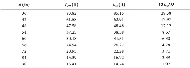
From the retention time constraint quantity, the various diameters and lengths combinations are shown in Table 4.
Given the slenderness ratio value which is must be between 3 and 4 to eliminate re-entrainment tendencies, the two-phase vessel selected is shown in Table 5.
3.2. Three Phase Process Vessel Sizing
1) Retention time is taken to be 1 min.
2) (ho)max is the maximum oil pad thickness that will permit the sized droplets
of water to settle to bottom of the vessel and permit the sized oil droplet to rise to oil-water interface and it is calculated to be 13.44 inch.
3) Aw
A represents the fraction of the vessel filled with water and calculated as
0.009.
4) ho/d is the ratio of the oil pad thickness (based oil production rate
envi-saged and fluid properties) to the diameter of the vessel and it is calculated as 0.48.
5) dmax= 277.
6) The gas capacity constraint value from
dLeff= 8.6390.
Apparently too small and will not govern design. 7) The liquid capacity constraint as determined from d2L
eff= 108630.
8) Since the oil and water retention time constraint governs, the Seam to Seam lengths for d and Leff combinations are tabulated in Table 6.
[image:12.595.211.538.541.655.2]Referencing the standard industrial sizes and considering the slenderness ra-tio, the valid size is given in Table 7.
Table 4. Retention time constraint governed d and L selection for a 2-phase separator.
Liquid Retention Time Constraint
D Leff Ls 12Lss/d
30 36 42 48 54 60 66
23.8 16.54 12.15 9.30 7.35 5.95 4.92
26.3 19.4 15.65
13.3 11.85 10.95 10.42
10.520 6.520 4.470 3.325 2.630 2.190 1.895
Table 5. Selected 2-phase process vessel size.
D Leff Ls 12Lss/d
48 9.30 13.3 3.325
Table 6. Liquid capacity constraint d and Leff combinations.
d (in) Leff (ft) Lss (ft) 12Lss/D
36 42 48 54 60 66 72 84 90
83.82 61.58 47.58 37.25 30.18 24.94 20.95 15.39 13.41
85.15 62.91 48.48 38.58 31.51 26.27 22.28 16.72 14.74
28.38 17.97 12.12 8.57 6.30 4.78 3.71 2.39 1.97
Table 7. Sized three phase process vessel.
D Leff Lss 12Lss/D
72 20.95 22.28 3.71
3.3. Simulation Results
The process flow diagram obtained from the Hysys simulation of the two stage separation is shown in Figure 1.
The two stage treatment process is comprised of a first two phase separator followed by a second stage three phase separation. The efficiency of the process is in the propensity to determine optimal operating pressures of the vessels. Thermodynamic properties of the fluid system have to be carefully altered to permit the desired phase separation. Table 8 and Figure 2 represent the material balance across the two phase separation stage and two phase molar flow recovery across the two phase separator respectively.
The Gas rate dropped from 132,918 Ibmole/hr to 128,652 Ibmole/hr (differ-ence of 4266 Ibmole/hr) because of high operating pressure in the vessel causing gas entrainment in the liquid stream. The liquid stream also increased from 8704 Ibmole/hr to 12,971 Ibmole/hr consequent upon the high operating vessel pres-sure validating the effectiveness of the operating prespres-sure selected.
Table 9 and Figure 3 represent the obtained material balance across the three phase separator and the molar flow recovery across the three phase separator respectively.
Here we observed all the compensations required to balance out materials. Entrained gas in liquid from two-phase separation was accounted for at 4375 Ibmole/hr. The flow rate of oil slightly increased by 270 Ibmole/hr as a result of low pressure of the separator causing lighter end hydrocarbon to condense into liquid oil while the water flow rate dropped by 359 Ibmole/hr. This also was due to flashing of the hydrocarbon content of the water feed stream.
4. Conclusions
The modeled equipment when sized with Mathlab gave standard sizes available in the industry today. The sized equipment was used to run the dynamic simula-tion of the two-stage separasimula-tion process. The multiphase fluid from the well
Figure 1. Aspen Hysys dynamic simulation of the two stage separation.
Figure 2. Phase recovery from 2-phase separator with operating pressure.
Table 8. Two phase material balance.
Unit Mixture Vapour Product Liquid Product
Vapour Fraction 0.907377905 1 0
Temperature F 120.1248562 118.2104249 118.2104249
Pressure Psia 900 850 850
Molar Flow lbmole/hr 141,624.0345 128,652.9011 12,971.13346 Mass Flow lb/hr 3,412,922.091 2,544,818.929 868,103.1621 Liquid Volume Flow USGPM 17,780.03815 14,978.78354 2801.254605
[image:14.595.210.539.604.729.2]Table 9. Three phase separator material balance.
Unit Liquid Product-1 Gas Oil Water
Vapour Fraction 0 1 0 0
Temperature F 118.210425 87.4358 87.4358 87.4358
Pressure psia 850 50 50 50
[image:15.595.209.539.90.208.2]Molar Flow lbmole/hr 12,971.1335 4375.621 7892.15 703.3626 Mass Flow lb/hr 868,103.162 122,325.7 733,106 12,671.52 Liquid Volume Flow USGPM 2801.25461 595.6206 2180.276 25.35793
Figure 3. 3-Phase recovery with operating pressure.
entered the two phase separator where about 96.77% of the gas flashed with the rest entrained with the liquid. The liquid from the first separator enters the second three-phase separator where the remaining 3.23% of the initial gas is flashed plus additional 0.083% light end hydrocarbons flashed. The oil and water were fully separated with additional 3.42% hydrocarbon recovery from other phases. The produced water from the process was treated to disposal standard in the produced water treatment unit whilst the gas was clear of droplets through the knock-out drum to the flare. The simulation and sized equipment results proved the ideality of the models.
For future works should include models for chemical injection and heating system(s) in case of hydrate and wax formation.
3-Phase Recovery
Operating Pressure
200 400
600 800
P
has
e
M
ol
ar
F
low
s
0 2000 4000 6000 8000 10000
Pressure Vs Gas Molar Flow
Pressure Vs Oil Molar Flow Pressure Vs Water Molar Flow
Conflicts of Interest
The authors declare no conflicts of interest regarding the publication of this paper.
References
[1] Atalla, F.S. and James, H.T. (2007) Modeling and Control of Three-Phase Gravity Separator in Oil Production Facilities. 42, 291-293.
https://www.academia.edu/9689973/Modeling_and_Control_of_Three-Phase_Gravi ty_Separators_in_Oil_Production_Facilities
[2] Amanat, C.U. (1999) Oil Well Testing Handbook. Petroleum Extension Service a Dictionary for the Petroleum Industry Third Edition.
[3] Arnold, K. and Stewart, M. (1999) Surface Production Operation: Design of Oil-Handling Systems and Facilities. 2nd Edition, Vol. 1, Butterworth-Heinemann, Woburn, MA.
[4] Williams Lyons, C. and Gary Plisga, J. Standard Handbook of Petroleum & Natural Gas Engineering. Vol. 2.
[5] Powers, M.L. (1990) Analysis of Gravity Separation in Freewater Knockouts. SPE Production Engineering, 5, 52-58. https://doi.org/10.2118/18205-PA
[6] API RP 45, 1998.
[7] Saeid, M. and Williams, P.A. (2012) Handbook of Natural Gas Processing and Transmission. Vol. 2.
[8] Schlumberger Well Test Manual. [9] API 12J, 1989.
![Table 3. Standard horizontal process vessel sizes [4] [9].](https://thumb-us.123doks.com/thumbv2/123dok_us/9109939.408226/11.595.211.536.87.679/table-standard-horizontal-process-vessel-sizes.webp)