Analytical Solution for Formation Flying Problem near Equatorial Circular Reference Orbit

(1)

ISSN Online: 2161-4725 ISSN Print: 2161-4717

DOI: 10.4236/ijaa.2019.93016 Aug. 30, 2019 217 International Journal of Astronomy and Astrophysics

Analytical Solution for Formation Flying

Problem near Equatorial-Circular

Reference Orbit

Shaheera A. Altalhi

1

, Magdy Ibrahim El Saftawy

1,2

1_{King Abdul-Aziz University, Jeddah, Saudi Arabia}

2_{National Research Institute of Astronomy and Geophysics, Helwan, Cairo, Egypt}

Abstract

The relative motion between multiple satellites is a developed technique with many applications. Formation-flying missions use the relative motion dy-namics in their design. In this work, the motion in invariant relative orbits is considered under the effects of second-order zonal harmonics in an equatori-al orbit. The Hamiltonian framework is used to formulate the problem. All the possible conditions of the invariant relative motion are obtained with dif-ferent inclinations of the follower satellite orbits. These second-order condi-tions warrantee the drift rates keeping two, or more, neighboring orbits from drifting apart. The conditions have been modeled. All the possibilities of choosing mean elements of the leader satellite orbit and differences in mo-menta between leader and follower satellites’ orbits are presented.

Keywords

Invariant Relative Orbits, Formation Flying Satellites, Relative Motion

1. Introduction

As the geostationary Earth orbits (GEO) belt becomes more crowded it is in-creasingly difficult to acquire slots for new satellites. Consequently, many or-ganizations choose to collocate their spacecraft in the same slot. Also for mis-sions which a single satellite cannot accomplish, as global position satellite sys-tem (GPS), the needed of formation flight began.

The formation flight concept is the use of several small satellites, which work together in a group (or constellation) to accomplish the objective of one larger, usually more expensive, satellite. This increases the likelihood of mission success in the event of a malfunction Hughes [1]. Formation flights have invariant

rela-How to cite this paper: Altalhi, S.A. and El Saftawy, M.I. (2019) Analytical Solution for Formation Flying Problem near Equatori-al-Circular Reference Orbit. International Journal of Astronomy and Astrophysics, 9, 217-230.

https://doi.org/10.4236/ijaa.2019.93016

Received: March 29, 2019 Accepted: August 27, 2019 Published: August 30, 2019

http://creativecommons.org/licenses/by/4.0/

(2)

DOI: 10.4236/ijaa.2019.93016 218 International Journal of Astronomy and Astrophysics

tive orbits for their satellites to ensure that they will not separate over time. The invariant relative orbits have been studied for a long time, as the earlier work of Clohessy and Wiltshire [2] in addition to the studies of Tschauner and Hempel [3]. These models introduced conditions on the initial relative position and velocity so that the relative orbits result to be periodic, which are closed or-bits. Recently, Schaub and Alfriend [4], Abd El-Salam et al.[5] passing through Li and Li [6] until Abd El-Salam and El-Saftawy [7] in which they discussed the invariant relative orbits due to the influence of the perturbative effects of the as-phericity of the Earth, the relativistic corrections and the direct solar radiation pressure. Rahoma [8] also, discussed the J2 invariant relative orbits with the

ef-fect of lunisolar attraction.

In this paper, we extend the works of Schaub and Alfriend [2] and Abd El-Salam et al.[5] model by introducing an atlas for the curves of invariant rela-tive orbits’ conditions. This atlas will be presented using Mathematica program to calculate and plot graphics of the initial conditions of invariant relative orbits. Those graphics will be shown as curves in 2D; in the case of the orbit of the leader satellite is equatorial.

2. Hamiltonian System

There are several ways to derive the equations of motion for any such system. We emphasized on the Hamiltonian structure of this system. The Hamiltonian formulation allows additional conservative forces to add to the Hamiltonian, thus the addition of complexity to the model can be incorporated with ease. Non-conservative forces can add in the momenta equations of motion. The Ha-miltonian equations of motion allow us to directly use control and simulation techniques.

After expressing the Hamiltonian, as a series in power of J2 (The second

geo-potential zonal harmonic) up to the second order, and using Lie-Deprit-Kamel perturbation method Kamel [9] to eliminate, in successive, the short and long periodic terms, the transformed Hamiltonian, H**_{, for different orders 0, 1, and}

2, are obtained by El-Saftawy et al.[10].

2

** ** ** 2 **

0 2 1 J₂ 2

H =H +J H + H (1) where,

2 **

0 ₂ 2,0

H = −µ η _(1.1)

(

)

** 2

1 11 3,3 3 2

H =A η _ − _(1.2)

(

)

(

)

(

)

(

)

(

)

2

** 11 4

2 2 1,9 3,7 4,6 5,5

2

1,9 3,7 4,6 5,5

$ 2

22 3,7 5,5

1 ₅₅₁₇ ₂₄₆ ₃₄₅₆ ₁₃₅

128

11520 2976 8064 672 4704 576 1536 288

3 ₅ ₃ ₃₅ ₄₀ ₈

2

A H

A

η η η η

µ

η η η η

η η



= _ − + − +

+ − + +



+ − + − + _

+ − − +

 

(3)

With, ηi j, =L L1−i −2j,  = SinI (I is the inclination of the orbit), μ is the

gra-vitational parameter of the planet and zero order quantities defined as:

4 2

11

6 4 4

22 2

2

, 4

. 32

e

r A

r J A

J

µ

=

where li and Li are the Delaunay elements (L1= µa, L2=L1

(

1−e2

)

,

3 2Cos

L =L I), re is the equatorial radius of the Earth, and J2, J4 are the second

and fourth geopotential zonal harmonic respectively.

The problem of designing invariant relative orbits for spacecraft flying forma-tions is outlined as follows:

1) Compute the secular drift of the longitude of the ascending node and the sum of the argument of perigee and mean anomaly.

2) These secular drift rates are set equal between two neighboring orbits. 3) Having both orbits drift at equal angular rates on the average, they will not separate over time due to the influence of the perturbative effects of the asphe-ricity of the Earth up to the desired order of magnitude (or the accuracy) to the equations of motion.

Using the canonical equations of motion,

** **

, , 1,2,3

i i

i

H H

l L i

L l

∂ ∂

= = − =

∂ ∂

  ₍₂₎

Since the argument of mean latitude θ_{is the sum of the mean anomaly and}

the argument of perigee (l1 + l2). Evaluating the derivatives yields the sum of the

argument of perigee and the mean anomaly rate of changes. Follows, the rate of change of mean latitude, θ_{, and the secular drift rates of the longitude of the}

ascending node, l3 can be calculated, i.e. θ  = +l l1 2.

So, using Equation (1) in Equation (2), the result can written in the form:

2 2 0 !

n n n

J n θ

θ = =

∑

 _{D and} 2 2 3

3

1 !

n l n n

J l

n

= =

∑

 _{D (3)}

With, D and θn Dln3 are published by Abd El-salam et al. [5] and given by:

0 2

0 K

θ ₌_µ

D

3

1l =A Z11 1

D

0 2

1 11

1

i K

A

θ

=

∑

D

2 5 7

11

2 2 22

2 6

3 3

128 i 2 i

i i

A _Z _A _Z

θ

µ = =

=

∑

+

∑

D

2 8 12

11

2 2 22

3 9

3 3

128 i 2 i

i K i K

A _A

θ

µ = =

=

∑

+

∑

D

where Ki and Zi are function of the action variable and introduced in Ap-pendix.

(4)

growth needs to be equal. So, it would be desirable to match all three rates l l 1 2,

and l3 between the satellites in each formation. So θ and l3 of all satellites

in the formation should be equal.

1, 2, 1, 2,

3, 3,

i i i j j j

i j

l l l l i j

l l i j

θ = + = + =θ ∀ ≠

= ∀ ≠

   

 

  (4)

Denoting the reference means orbit elements with the subscript “0”. Using Taylor expansion for the drift rate θi and l3,i of a neighboring orbit “i” about

the reference orbital elements, retaining the terms up the second-order deriva-tives, can be simplified as:

0 0 0

1,1 1

1 2 3

1,0 1,1 2,1

2 3 3

2 2 2 2

2 2,2

2 2 2

2

1 2 3

1 ₂

2

i i i

i

x x x x x x

i i i

x x x x x x

i i i i

x x x x x x

L

L L L

I

L L L

L

L L L

θ θ θ

δθ η δ

θ θ θ

η δη η δ

θ _η θ θ θ

− = = = − − − = = = − = = = _∂ _∂ _∂     = + +   ∂ ∂ ∂  _ _   _∂ _∂   _∂      + + − ∂ ∂ ∂         ∂ ∂ ∂ ∂ + + + + ∂ ∂ ∂ ∂                

( )

(

)

( )

0

0 0 0

3

2 2 2

2

1,1 1 2,0 2

1 2 1 3 2

2 2 2

2 2

1,1 4,2

2 2

2 3 3 3

1 2 2 1 2 2 x x

i i i

x x x x x x

i i i

x x x x x x

L

L L L L L

I

L L L L

θ θ θ

η δ η

θ θ _δη _η θ _δ

= − − = = = − − = = =        ∂   _ _    _∂ _∂  _∂     + + + ∂ ∂ ∂ ∂  ∂       ∂ ∂ _ _ ∂ _ + + + ∂ ∂ ∂ _ _ ∂ _          

( )

(

)

( )

(

)

0 0 0

0 0

0

2 2 2

2

2,1 2 2

2 3

2 2

1,0 1 1,1

1 2 1 3

2 2

3,1 2 1,1

2 3 3 2 3,2 2 3 2

i i i

x x x x x x

i i

x x x x

i i

x x x x

i x x

L L

L L

L L L L L

I L L

L

θ θ θ

η

θ θ

η δ δη

θ θ

η δ δη

θ η − = = = − − = = − − = = − =  _∂ _∂ _∂     + + +  ∂ ∂   _∂ ∂ _    _∂ _∂     + + ∂ ∂ ∂ ∂     _∂ _∂    − − ∂ ∂ ∂     ∂ − + ∂               

( )( )

0 0 2 2 2,1 1

2 3 1 3

i i

x x x x

L I L L L L

θ _η θ _δ _δ

− = =   _∂  _∂    +   ∂ ∂  ∂ ∂  _ _ _    (5)

With  = CosI, similarly:

0 0 0

0 0

3, 3, 3,

3, 1,1 1

1 2 3

3, 3, 3,

1,0 1,1 2,1

2 3 3

2 2 2

3, 3, 2 3

2,2

2 2

1 2

1 1

2 2

i i i

i

x x x x x x

i i i

x x x x x x

i i

x x x x

l l l

l L

L L L

l l l

I

L L L

l l l

L L

δ η δ

η δη η δ

η − = = = − − − = = = − = = _∂ _∂ _∂     = + + ∂ ∂ ∂      _∂ _∂   _∂      + + − ∂ ∂   ∂      ∂ ∂ ∂ + + + ∂ ∂               0 0 2 , 3, 2 2 3 3 2 i i

x x x x

l L L

L ₌ ₌

(5)

( )

(

)

( )

0 0 0

0

2 2 2

2

3, 3, 3,

1,1 1 2,0 2

1 2 1 3 2

2 2 2

2 2

3, 2 3, 2 3,

1,1 4,2

2 2

2 3 3 3

2 2

3, 2 3,

2,1 2 2 1 2 1 2 2

i i i

x x x x x x

i i i

x x x x x x

i x x

l l l

L

L L L L L

l l l

I

L L L L

l l

L

η δ η

δη η δ

η − − = = = − − = = = − =   _∂ _∂  _∂     + + +  ∂ ∂ ∂ ∂  ∂       ∂ ∂ _ _ ∂ _ + + +    ∂ ∂ ∂ ∂    ∂ ∂ + + ∂              0 0 2 3, 2,1 2 2 3 3 2 i i

x x x x

l L L L η−

= =   _∂    ₊    ∂ ∂ ∂      

( )

(

)

( )

(

)

0 0 0 0

0 0 0

2 2

3, 3,

1,0 1 1,1

1 2 1 3

2 2

3, 3,

3,1 2 1,1

2 3 3

2 2 2

3, 3, 3,

3,2 2 2,1

2 3 1 3

3

i i

x x x x

i i

x x x x

i i i

x x x x x x

l l

L L L L L

l l

I L L

L

l l l

L L L L L

η δ δη

η η − − = = − − = = − − = = =   _∂ _∂     + +  ∂ ∂ ∂ ∂     _∂ _∂    − +  ∂ ∂ ∂      _∂ _∂  _∂      − + +  _ ∂ ∂ ∂ _ ∂ ∂ _           

  _

( )( )

δL1 δI

(6)

where δθi = −θ θ i 0 is the difference between the drift rates of the argument of

mean latitude of the reference orbit and one of the neighboring orbits, and

0 0

i X X

θ θ

= =

  _.

And δl3,i=l3,i−l3,0 is the difference between the drift rates of the ascending

node of the reference orbit and one of the neighboring orbits, and

0

3,_{i X X} 3,0

l ₌ =l _.

Now, the conditions satisfying the invariance property for the relative orbits are:

0 0

i i

δθ = −θ θ  = (7)

3,i 3,i 3,0 0

l l l

δ = − = ₍₈₎

Substituting the included derivatives of the last two equations into Equations (5) and (6) and after the needed mathematical manipulations we will get:

(

)

( )

(

)

(

)

(

)

( )

(

)

( ) (

)

1 1 1

1 1

2

2 2

1 1, 1 1 1, 1

1, 1 1 0

L L I II L

I L L I

A L A I A I A A L A A I A A I L

θ θ θ θ θ

ηη η

θ θ θ θ

η η

δ δ δ δη δ δη

δ δη δ δ

− − −   +_ + _+ +    

+_ + _ +_ + _ = (7')

( )

(

)

( )

(

)

( ) (

)

( ) ( )

3 3 3 3 3

1 1 1

3 3

1 1

2

2 2

1 1, 1 1 1, 1

1. 1 1 0

l l l l l

I II

L L L

l l

I L L I

A L A I A I A A L A A I A A I L

ηη η

η η

δ δ δ δη δ δη

δ δη δ δ

− − −   +_ + _+ +    

+_ + _ +_ + _ = (8')

Multiplying Equation (7') by 3 1 1

l L L

A and Equation (8') by AL Lθ_{1 1} and subtract-ing we will get:

(

)

2

1 1 1, 1 2 1, 1 3 1 4 1, 1 5 0

a Lδ δη ₋ +a δη ₋ +a L aδ + δη ₋ +a = ₍₉₎

with the coefficients ai’s are:

3 3

1 1 1 1 1 1

1 L L Ll Ll L L

a θ θ

η η

(6)

3 3

1 1 1 1

3 3

( )

3

( )

1 1 1 1

2 2

5 I II L Ll L L Il IIl

a ₌_ θ _δI ₊ θ _δI _ ₋ θ _δI ₊ _δI

      

and the derivatives of _θ_{’s and} _l3’s are in the appendix. Solving Equation

(9), for δL1, we get:

(

)

2

2 1, 1 4 1, 1 5

1

1 1, 1 3

a a a

L a a δη δη δ δη − − − + + = − +

Substituting the last results in Equation (7') we get the quartic equation:

(

)

4

(

)

3

(

)

2

(

)

1 1, 1 2 1, 1 3 1, 1 4 1, 1 5 0

b δη ₋ +b δη ₋ +b δη ₋ +b δη ₋ +b = _,

where the coefficients bi’s are functions of Li’s and given by:

1 1 1

2 2

1 2 L L 2 1 L 1

b a θ a a θ a θ

η ηη

=  −  + 

(

)

( )

1 1 1 1 1

2 2 4 2 3 1 4 2 1

2

1 1 3

2

L L L L IL

I

b a a a a a a a a I

a I a a

θ θ θ θ

η

θ θ θ

η η ηη

δ δ   = − + −     +   + + +       

(

)

(

)

(

)

( )

1 1 1

1 1

2 2

3 4 2 5 4 3 5 1 3

2 3 1 4 1 3

2 2

1

2

L L L

L IL I

I II

b a a a a a a a a

a a a a I a a I

a I I

θ θ θ

η ηη

θ θ θ θ

η η θ θ δ δ δ δ     = + − + +   − + _ + _+ + + _ + _         

(

)

( )

1 1 1 1 1

4 4 5 5 3 4 3 5 1

2 2

3 3 1

2

L L L L IL

I I II

b a a a a a a a a I

a I a a I I

θ θ θ θ

η

θ θ θ θ

η η

δ

= − − +    + + _ + _+ _ + _        

( )

1 1 1 1

2

2 2

5 5 L L 5 3 L IL 3 I II

b ₌a θ ₋a a _ θ ₊ θ _δI _₊a _ θ _δI ₊ θ _δI _

   

    

Solving the resulting equation we will get four roots of δη1, 1− :

(

)

(

)

1, 1 _1,2 1 2 3

1, 1 _3,4 1 2 4

, .

δη

− − = − = +  

A A

A

A A

A

(10)

and four roots of δL1:

( )

(

₍

)

₎

(

)

( )

(

₍

)

₎

(

)

( )

(

₍

)

₎

(

)

( )

(

)

2 5 1 2 2 3 1 3 4 1 2 3 5

1 1

1 1 2 3 3

2 5 1 2 2 3 1 3 4 1 2 3 5

1 2

1 1 2 3 3

2 6 1 2 2 3 1 3 4 1 2 3 5

1 3

1 1 2 3 3

2 6 1 2 2 3 1 3 4

1 4

2 2 2

,

2 2 2

,

2 2 2

,

2 2 2

a a a

L

a a

a a a

L

a a

a a a

L a a a a L δ δ δ δ − + − + − − + = − − − + − − + + − − + = − − − + + − − + + − + = − + − + + + + + = −

A A A A A A A A A A

A A A

A A A A A A A A A A

A A A

A A A A A A A A A A

A A A

A A A A A A A

(

A

)

(

)

1 2 3 5

1 1 2 3 3

, a a a + − + + − + A A

A A A

(7)

where,

2 1

1

4

b b

= −

A , A2 =1₂ B B1+ 2+B3, A3=1 2₂ B B1− 2−B B3− 4 ,

4=1 2₂ B B1− 2−B B3+ 4

A , 2 2 2

5= 1 + 2 + 3

A A A A , 2 2 2

6= 1 + 2 + 4

A A A A ,

2 3 2

1 2

1 1

2 3 4

b b B

b b

= − , 1 3 1 2

1 4

2 3

C B

b C

= , 4

3 1 3

1

3 2

C B

b

=

× , 4 2 2

8

C B =

A ,

2

1 3 3 2 4 12 1 5

C =b − b b + b b _, 23 2 3 4

2 3 2

1

1 1

4b b 8

b b

C

b b b

= − + − ,

3 2 2

3 2 3 9 2 3 4 27 1 4 27 2 5 721 3 5

C = b − b b b + b b + b b − b b b _,

( )

(

)

1

3

3 2

4 3 4 1 3

C = C + − C +C _.

3. Modeling of Invariant Relative Orbit Conditions for near

Equatorial-Circular Case

When we choose the leader orbit to be circular equatorial then, we will obtain four solutions for δη1, 1− (which we redefined as δη for simplicity), as in

Equ-ation (10), and four solutions for δL1 as in Equation (10'). Here, we will

present the plots of these solutions, which we obtained in the last section (Equa-tions (10) and (10')) to compare the effect of J4 on the conditions of invariance

for the formation. Before we introduce the graphs, it is important to mention that in all figures, we provided a set of curves in each condition for the inclina-tion of each member of the formainclina-tion with respect to the leader orbit

(

− ≤2 δI≤2

)

_{as example. By means that the follower satellites’ orbits, in the}

formation, will be inclined by a range of 2˚ with respect to the leader satellite or-bit, of course we can extend this range. Also, we will introduce a comparison between the effects of J4 in the formation.

The variation of the formation relative to the leader orbit in δη_{is related to}

the variation in eccentricity for the followers through:

( )

2

1

e _{e MAG e e} e

δη= − δ = δ

− ,

i.e. the variation in the follower’s orbit in η1, 1− (δη) is scaled by MAG e

( )

in their variations in eccentricities δe_{. It is important to note that the scale}

function MAG e

( )

is always negative for circular and elliptical orbits. In our case the eccentricity of the leader orbit, e0, is zero, then δ = −e e e0 is always

positive.

While the variation in the δL1, for the followers, is scaled by mag a

( )

for

the variation of the semi-major axis through the relation

( )

1 ₂ 1

L a mag a a a

δ δ δ

µ

= = . It is important to note that the scale function

( )

(8)

3.1. The First Solution (Circular Formation)

The first solution of Equations (10) for δe and (10') for δa for the orbits of the followers with respect to the leader orbit, for inclination range [−2˚, +2˚] in case of J2 and the net effects of J2 and J4 can represent in the following curves.

Figure 1(a) and Figure 1(b) show the first choice of the invariant relative conditions, in the equatorial-circular case. In this choice, δη_and δL₁_get

Zero for all

δ δ

a e, _and δI _{values. That is mean, the formation for the}

fol-lowers orbit will be in the same orbital plane of the leader satellite (In Plane Circular Formation) with their eccentricities and semi-major axis was scaled by

( )

MAG e and mag a

( )

of the leader satellite. The scale function MAG e

( )

, for this solution, is equal zero whatever the choosing the value of δe. Also the scale function mag a

( )

never equal zero, then δa must equal zero. That can me conclude that the follower satellite’s must be in the same orbit of the leader one.

In this case, the effect of J4 has no significant variation in the formation.

3.2. The Second Solution

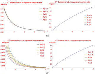
Figure 2(a) and Figure 2(b) show the second choice of the invariant relative formation, in the equatorial-circular case. In this solution, the choice of eccen-tricites and semi-major axis for the followers orbit is not affect the formation in case of J2 effect whatever choosing the inclination for folowers orbits. But the J4

effects change the choosing of eccentricities slightly while the choosing the semi-major axis still unaffected whatever chosing the inclinations for the fol-lowers orbits. As we see in the vertical axis. The semi-magor axis and eccentri-cites of the followers orbits must be greater than those for the leader one.

(a)

(b)

[image:8.595.219.525.442.681.2]

(9)

(a)

[image:9.595.211.533.69.321.2]

(b)

Figure 2. (a) The formation under the effect of J2 only for the 2nd solution in the circular equatorial of the leader orbit; (b) The formation under the net effect of J2 and J4 for the 2nd solution in the circular equatorial of the leader orbit.

The effects of J4 are changing slightly while the choosing of eccentricies is not

for choosing the semi-major axis.

3.3. The Third Solution

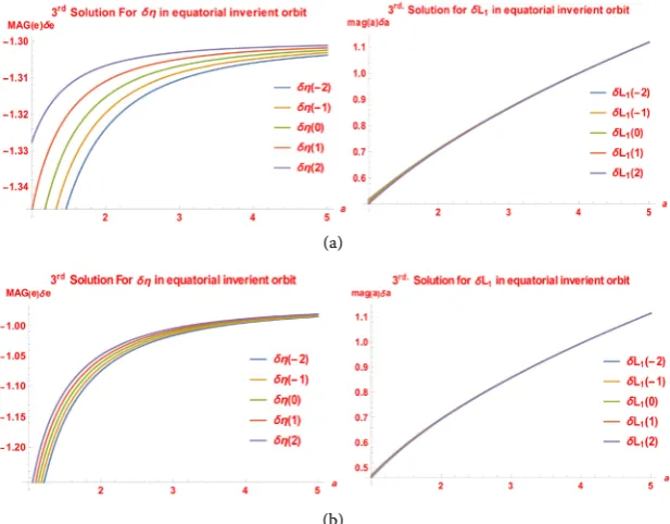
Figure 3(a) and Figure 3(b)show the third choice of the invariant relative for-mation, in the equatorial-circular case. In this solution, the value of the function

( )

1.3

MAG e eδ < − _{which gives the limits for the eccentricities through the}

inqu-alety _e4₊_1.69_e2₋_{1.69 0}_ _.

The solution for this inqualety has only one positive value 0.839936. With re-spect to choosing the semi-major axis, it is not depend on choosing the inclina-tion, by mean that the formation will be in plane of the leader one.

In the case of the formation, under the effects of J2 and J4, the function

( )

MAG e eδ _{is modified the limit of the eccentricities to be 0.774904.}

3.4. The Fourth Solution

Figure 4(a) and Figure 4(b) show the fourth choice of the invariant relative formation, in the equatorial-circular case. In this choice, the formation for def-ferent inclination is distributed about the leader orbit (with δI=0) and the function MAG e e

( )

δ _{is increasing for positive}δI_{while it is decreasing for}

negative δI. For choosing the semi-major axis, it increases by increasing the semi-major axis of the leader orbit whatever choosing δI .

In this formation choics, the effect of J4is significant for choosing the

(10)

(a)

[image:10.595.219.528.71.312.2]

(b)

Figure 3. (a) The formation under the effect of J2 only for the 3rd solution in the circular equatorial of the leader orbit; (b) The formation under the net effect of J2 and J4 for the 3rd solution in the circular equatorial of the leader orbit.

(a)

[image:10.595.217.531.376.621.2]

(b)

Figure 4. (a) The formation under the effect of J2 only for the 4th solution in the circular equatorial of the leader orbit; (b) The formation under the net effect of J2 and J4 for the 4th solution in the circular equatorial of the leader orbit.

Figure 4(b), the function MAG e e

( )

δ _{is positive and increasing while} MAG e

( )

(11)

Also, the second of Figure 4(b) shows that this choice is not continuous for orbits with semi-major axis greater than 2.5 earth radii. And the function

( )

mag a aδ is decreasing by increasing the semi-major axis.

4. Conclusions

The problem formulated using the oblate Earth model, truncating its potential series at J4 to the equations of motion, and then the canonical equations of

mo-tion and the Hamiltonian formed. In order to keep the relative momo-tion invaria-ble, eight-second order conditions between the differences in the semi-major axis a and the inclination I are obtained. These conditions guarantee that the drift rates of neighboring orbits are equal on the average. The resulting orbits require less control and maintenance fuel. Then we studied the curves of these conditions in equatorial-circular case. The plots of these cases are presented as relations between δη_or δL₁_{and the semi-major axis of the leader satellite}

orbit, at different δI.

In the first choice, we can conclude that the follower satellite’s must be in the same orbit of the leader one (on orbit formation).

In the second choice, whatever the choosing the inclination for the followers it is not affect the choosing the semi-major axis (In plane with different eccentrisi-ties).

The third choice, under the effects of J2 and J4, the value of the function

( )

1.3

MAG e eδ < − _{which gives the limits for the eccentricities through the}

in-equality _e4₊_1.69_e2₋_{1.69 0}_ _{. The solution for this inqualety has only one}

posi-tive value 0.839936. With respect to choosing the semi-major axis, it does not depend on choosing the inclination, by mean that the formation will be in plane of the leader one.

The fourth choice, the function MAG e e

( )

δ is positive and increasing while

( )

MAG e is always negative. And δe, in our case, must be positive or zero. For that, the eccentricities of the followers must be negative and that is not mathe-matically accepted.

Also, the second of Figures 4(b) shows that this choice is not continuous for orbits with semi-major axis greater than 2.5 earth radii. And the function

( )

mag a aδ is decreasing by increasing the semi-major axis.

Conflicts of Interest

The authors declare no conflicts of interest regarding the publication of this pa-per.

References

[1] Hughes, S.P. (1999) Formation Flying Performance Measures for Earth-Pointing Missions. MSc Thesis, Blacksburg, Virginia.

[2] Clohessy, W.H. and Wiltshire, R.S. (1960) Terminal Guidance System for Satellite Rendezvous. Journal of the Aerospace Sciences, 27, 653-658.

(12)

[3] Tschauner, J. and Hempel, P. (1965) Rendezvous Zueinem in Elliptischer Bahn Umlaufenden Ziel. Acta Astronautica, 11, 104-109.

[4] Schaub, H. and Alfriend, K. (2001) J2 Invariant Relative Orbits for Spacecraft For-mations. Celestial Mechanics and Dynamical Astronomy, 79, 77-95.

https://doi.org/10.1023/A:1011161811472

[5] Abd El-Salam, F.A., El-Tohamy, I.A., Ahmed, M.K., Rahoma, W.A. and Rassem, M.A. (2006) Invariant Relative Orbits for Satellite Constellations: A Second Order Theory. Applied Mathematics and Computation, 181, 6-20.

https://doi.org/10.1016/j.amc.2006.01.004

[6] Li, X. and Li, J. (2005) Study on Relative Orbital Configuration in Satellite Forma-tion Flying. Acta Mechanica Sinica,21, 87-94.

https://doi.org/10.1007/s10409-004-0009-3

[7] Abd El-Salam, F.A. and El-Saftawy, M.I. (2012) Second Order Constraints in the Theory of Invariant Relative Orbits Including Relativistic and Direct Solar Radia-tion Pressure Effects. Indian Journal of Science and Technology, 5, 1-14.

[8] Rahoma, W.A. (2013) Lunisolar Invariant Relative Satellite Orbits. American Jour-nal of Applied Sciences, 10, 307-312.https://doi.org/10.3844/ajassp.2013.307.312

[9] Kamel, A.A. (1969) Expansion Formulae in Canonical Transformations Depending

on a Small Parameter. Celestial Mechanics, 1, 190-199. https://doi.org/10.1007/BF01228838

(13)

Appendix

1 2 2 0 ! n L n n J n θ θ =   =    

∑

  , 2 2

1 ! n n n J n θ η θ =   =    

∑

  , 2 2

1 ! n I n n J n θ θ =   =    

  , 1 2 2 1 ! L n n n J n θ θ η =   = _ _  

∑

  , 2 2

1 ! n I n n J n θ θ η =   = _ _  

∑

  , ₁ 2 2

1 !

n n n

ILθ J_n θ

=   = _ _  

∑

  . 3 3 1 2 2 1 ! n l n n l

L J_n

=

 

=  

 

∑

  , 3 2 2 3

1 ! n l n n l J n η =   =    

∑

  , 3 2 2 3

1 ! n l n n l

I J_n

=   =    

∑

  , 3 3 1 1 2 2 1 !

l n l

n n

L L J_n

=

 

=  

 

∑

  , 3 2 2

  . With, 0 0 1 L

θ ₌∂ θ

∂

 D ,

2

1, 1 1, 1

1 3

n n n

n _L _L _L

θ θ θ

θ _η _η

− −

=∂ + ∂ + ∂

∂ ∂ ∂

 D D D ,

2 3

1 1

n L _Ln L _Ln

θ θ

θ ₌ ∂ ∂

∂ +  ∂

 D D ,

2 3

n

n L _L

θ ∂ θ

∂ = − 

 D ,

2

0

1 1 0

1 2 L L

θ

θ ₌ ∂

∂ ∂

 D ,

2 2 2 2

2 2, 2

1 1 2 2 3 3 2 3

2 2

3 2

1, 1

1 1

1 1 ₂

2 2 n n

n

n n n

n

L L L L L L L L

L L L L

θ θ θ θ θ

θ θ η η − − ∂ ∂ ∂ ∂ ∂ ∂ ∂ ∂ ∂ ∂ ∂ ∂  ∂ ∂   _{∂ ∂}    = + _ + + _   + + ∂ ∂     

 D D D D

D D ,

2 2

2 2 3 3 2

1

3 2

1 ₂

2 n

n L _{L L} _{L L}n _{L L}n

θ θ θ

θ  ∂ ∂ ∂ 

_{∂ ∂} _∂ 

= + +

∂ ∂ ∂

   

 D D D ,

2 2

3 3 0, 2

1

2 n

n _{L L}

θ θ _η − ∂ ∂ ∂ = _

 D ,

2 2 2 2 2

2

2 2 3 3 2 3 1 2 1 3

2

1

2

n n n n n

n L _{L L} _{L L} _{L L} L _{L L} _{L L}

θ θ θ θ θ

θ  ∂ ₊ ∂ ₊ ∂  ∂ ₊ ∂

_{∂ ∂} _{∂ ∂} _{∂ ∂}  _{∂ ∂} _∂  = _{+ } ∂        

 D D D D D ,

2 2

3 3 1,

2 3

1 n

n _{L L}n _{L L}

θ θ θ _η − −   = − ∂ + ∂ ∂ ∂   ∂   ∂  

(14)

2 2 2

3 3

1, 2 1,

2 3 1 1 3

n n n

n _{L L} _{L L} _{L L}

θ θ

θ _η θ _η

− −  ∂ ∂ ∂  + +  _{∂ ∂} _∂  = − ∂ ∂ ∂    

 D D D ,

3 3 3

3

1, 1 2

1 3

n n

l l l

l

n _L η − _L _Ln

 

=∂ + ∂ + ∂ ∂ _∂  ∂ _

 D D D ,

3 3

3

1

2 3

n l

l l n

n L _L _L

 

= ∂ + ∂

∂ ∂

 

  

 D D ,

3 3 2 3 n l l

n L _L

∂ =

∂ − 

 D ,

3 3 3 3

3 3 3 2 2 2 2, 2 1 1 1, 1 1 1 2 2

2 2 3 3 2 3

2 2

2 3

1 1

2 n 2 n n 2

l l l l

l n

n ln

n

l

L L L L L L L L

L L L L

η η − − ∂ ∂ ∂ ∂ + + ∂ ∂ ∂ ∂ ∂ ∂   = ∂ ∂ ∂ ∂  + _{∂ ∂} _{∂ ∂}  + _   +      

 D D D D

D D ,

3 3 3

3 2 2

1

2 2 2

2 2 3 3 2 3

1 ₂

2

l l

n l

l

n L _{L L}n _{L L} _{L L}n

 

= ∂ + ∂ + ∂

∂ ∂ ∂ ∂ ∂ ∂ _ 

  

 D D D ,

3 3 2 2 3 3 2 2 1 2

l ln

n L _{L L}

∂ ∂ =

∂ 

 D ,

3 3 3 3 3

3

2 2 2 2 2

2

2 2 3 3 2 3 1 2

2

1

1 3

2

n

l l l l l

l n n n n

n L _{L L} _{L L} _{L L} L _{L L} _{L L}

  = _ + + _+ +     ∂ ∂ ∂ ∂ ∂   ∂ ∂  ∂ ∂ ∂ ∂ _∂ ∂ ∂ ∂ _

 D D D D D ,

3 3

3

2

3 3 2 3

1,

2

1 n

l l ln

n η− − _{L L} _{L L}

∂ ∂ ∂ ∂   = − + ∂     ∂ 

 D D ,

3 3 3

3

2 2 2

3 3 2

1, 2 1

3 ,1 1 3

l l l

n

l n n

n η − _{L L} _{L L} η− _{L L}

∂ ∂ ∂ ∂ ∂ ∂   = − _ + + ∂  ∂ ∂   

 D D D ,

12 945 630 45 5,6

K = _ − _ + η _,

and,

7 420 180 5,6